Multi-Objective Robust Optimization of Integrated Energy System with Hydrogen Energy Storage

Abstract

A novel multi-objective robust optimization model of an integrated energy system with hydrogen storage (HIES) considering source–load uncertainty is proposed to promote the low-carbon economy operation of the integrated energy system of a park. Firstly, the lowest total system cost and carbon emissions are selected as the multi-objective optimization functions. The Pareto front solution set of the objective function is applied by compromise planning, and the optimal solution among them is obtained by the maximum–minimum fuzzy method. Furthermore, the robust optimization (RO) approach is introduced to cope with the source–load uncertainty effectively. Finally, it is demonstrated that the illustrated HIES can significantly reduce the total system cost, carbon emissions, and abandoned wind and solar power. Meanwhile, the effectiveness of the proposed model and solution method is verified by analyzing the influence of multi-objective solutions and a robust coefficient on the Chongli Demonstration Project in Hebei Province.

1. Introduction

Countries around the world are actively exploring more low-carbon and economical energy utilization methods to alleviate the global energy crisis and environmental pollution [1,2]. Hydrogen energy storage (HES) is characterized by high energy density and a non-polluting use process. Therefore, HIES has become one of the most important direction for the development of low-carbon economies in future integrated energy systems (IES) [3,4]. In addition, the increasing variety of energy sources used in IES poses a great challenge to optimizing the operation of IES in low-carbon economies [5,6]. Therefore, the study of the optimal operation of these systems has become a hot topic in the energy field.

In recent years, a great deal of research has been conducted on optimizing the operation of hydrogen IES. The authors of [7] introduced an electric hydrogen production unit into a microgrid and developed a real-time operation optimization model. The authors of [8] presented a two-stage optimal selection method for an isolated electric hydrogen heating–cooling cogeneration IES and verified the economic advantages of IES with seasonal hydrogen storage. The authors of [9] proposed an optimal operation scheme for electric hydrogen heating, which improved the economy and safety of the system. The optimization objectives established in the literature [7,8,9] are all single objectives. However, in the context of the low-carbon transition of the energy system, conventional single-target economic dispatch has experienced difficulties in meeting the optimization requirements, and the carbon emissions of the system have become an important part of the optimal operation of IES [10]. For this reason, the studies in [11,12,13,14] examined the multi-objective optimization of IES. The author of [11] proposed an IES that includes hydrogen and renewable energy sources, and a multi-objective optimal scheduling model was developed by considering the economic and environmental benefits. The authors of [12] proposed an integrated natural gas–wind–photovoltaic–hydrogen energy system with a multi-objective optimization model, considering its annual integrated cost and carbon emissions. A multi-objective optimization model of a wind–hydro–hydrogen power generation system was developed in [13]. The authors of [14] established a multi-objective optimization strategy in which carbon emissions were better than the total cost, in order to further reduce the carbon emissions of the system for the first time.

Multi-objective solving is a complex process, and commonly used methods include the ε-constraint method [15], the non-dominated sequential genetic algorithm-II (NSGA-II) [16,17], the multi-objective particle swarm algorithm (MOPSO) [18,19], and the multi-objective genetic algorithm (MOGA) [20]. However, these algorithms always have certain limitations; for example, the efficiency and completeness of the solution of NSGA-II will be affected by the size of the population, and MOPSO is computationally complex and has poor convergence.

In addition, there are uncertainties in the different energy systems involved above, such as wind power, photovoltaics, and loads, which can adversely affect the optimal operation of HIES [21,22]. However, these uncertainties are not considered in the above studies. To cope with the uncertainty, the following methods are commonly used: stochastic optimization (SO) [23,24], RO [25,26], fuzzy optimization [27], and interval optimization [28]. Among these, SO and RO are the most widely used. The authors of [29] proposed an SO framework for multi-energy systems, aiming to address multiple uncertainties in renewable energy sources, tariffs, and loads. The authors of [30] described the uncertainty of energy sources such as wind, photovoltaic, electricity, heat, cold, and hydrogen based on stochastic scenario generation. The authors of [31] developed a hydrogen-based RO scheduling model for smart micro-energy centers, aiming to reduce the cost of the risk associated with electricity price uncertainty through RO. The authors of [32] proposed an RO model for a microgrid, considering uncertainty to balance the economics and robustness of its operation. The authors of [33] used a data-driven two-stage distributed robust optimization (DRO) approach to cope with the uncertainty of electric vehicles. On this basis, the authors of [22] proposed a framework for multi-objective optimization and robustness analysis by combining multi-objective optimization and two-stage SO. The authors of [34] proposed a multi-objective SO model to balance the economics and environmental friendliness of a system under multiple uncertainties. In a recent study, a novel robust multi-objective optimization model was proposed for islanded data center microgrids (DCMGs) [35].

In fact, when SO is employed to cope with uncertain disturbances, a large number of stochastic scenarios need to be generated, which is computationally more complex, especially when faced with a multi-objective problem [21]. In contrast, RO does not require information about the probability distribution of the determinant and only requires upper and lower bounds on the uncertain parameters, which is more efficient but may also lead to overly conservative decisions. DRO improves the conservatism of traditional RO decisions, but its transformation solution is complex and it may be less efficient when applied to large-scale IES uncertainty optimization [36]. To summarize the unique features of the proposed model compared to previous work in the field, a detailed comparison of the reviewed articles is further presented in Table 1.

Table 1. Comparison of different research methods.

Literature	Application System	Optimization Objectives	Optimization Tools	Uncertainty Handling
[7]	Microgrid with a power-to-hydrogen device	Minimize operating cost	Mixed-integer linear programming	×
[8]	Island IES combined power–hydrogen–heat–cooling cogeneration	Life cycle cost	Random-trigonometric grey wolf	Clustering and scenario generation
[9]	Active distribution networks + heat to district heating networks + power-to-hydrogen-and-heat scheme	Minimize operating cost	CPLEX	RO
[11]	Wind turbine + photovoltaic cell + electrolytic hydrogen + fuel cell + hydrogen storage	Operating cost + carbon footprint	NSGA-II	×
[12]	Natural gas–wind–photovoltaic–hydrogen IES	Annual consolidated cost + annual carbon emissions	The branch and bound procedure	×
[13]	Grid-connected photovoltaic–hydrogen–natural gas IES	Annual total cost + annual carbon emissions	The branch and bound procedure	×
[14]	Wind–solar–water–hydrogen IES	Minimum loss of daily load + maximum net annual income + carbon footprint	Twin delayed deep deterministic policy gradient algorithm	×
[22]	CCHP-based renewable auxiliary BIES system	Total annual cost + annual carbon emissions	Enhancement of epsilon constraint	Two-stage SO
[29]	Multi-energy hub systems	Minimize operating cost	BONMIN	SO
[30]	A grid-connected electricity–hydrogen integrated energy system	Minimize operating cost + carbon footprint + energy losses	Improved multi-tasking and multi-objective optimization	Scene generation
[31]	Hydrogen-based smart micro energy center	Total cost minimization	Strong duality theory	RO
[32]	Micro-grid	Operating cost	The Benders dual algorithm	RO
[33]	IES, electricity–hydrogen hybrid charging station	Maximize revenue	Bisection-based distributed algorithm combined with the C&CG algorithm	DRO
[34]	Multi-renewable hybrid CCHP systems	Total annual cost + environmental indicators	NSGA-II	SO
[35]	DCMG	Total operation cost wind + power curtailments + computation resource over-plus level	Epsilon constraint	RO
This paper	HIES	Total system cost + carbon emissions	Compromise planning	RO

The results of the studies are summarized by comparing the related literature: although there has been some development in considering multi-objective optimization regarding HIES in the existing work, the efficiency and accuracy of their solutions need to be improved. Meanwhile, the previous studies lack a comprehensive consideration of the system uncertainty. Moreover, as of now, there is little research on the multi-objective robust optimization of HIES considering the source–load uncertainty.

A multi-objective robust optimization model for HIES considering source–load uncertainty is proposed in this paper to fill the gap in the existing research. RO is adopted to deal with the system uncertainty, and compromise planning and max–min fuzzy methods are applied to solve the model. Finally, the model is validated by practical arithmetic examples. The main contributions are summarized below.

• A HIES multi-objective robust optimization model considering source–load uncertainty is proposed to balance the economy and environmental protection of the system operation under multiple uncertainties.
• The compromise planning and max–min fuzzy methods are applied to solve the multi-objective robust optimization models and to obtain the Pareto frontier solutions and its optimal solutions. Compared with the widely used NSGA-II, the compromise programming method has a larger search space and more uniform frontier solutions.
• The modified RO method used to ameliorate the source–load uncertainty improves the system’s ability to cope with the uncertainty risk, and the multi-objective RO is more efficient than the multi-objective SO. The system’s features are regulated by adjusting the robustness coefficient, which overcomes the strong conservatism of the traditional RO.

2. HIES Modeling

2.1. Schematic of HIES

This paper adopts the HIES structure shown in Figure 1, which is based on the Chongli Large-Scale Wind–Solar Complementary Coupled Hydrogen Production System Application Demonstration Project. The system includes a wind turbine (WT), photovoltaic (PV) and combined heat and power (CHP), a gas boiler (GB), a heat pump (HP), electrolytics (EL), a hydrogen fuel generator (HFG), an electric cooler (EC), an absorption cooler (AC), and electric storage (ES), heat storage (HS), cold storage (CS), and HES, which are categorized as four types of energy storage equipment.

Figure 1. Schematic of HIES.

When the system is in normal operation, CHP, GB, and HP supply the heat to meet the heat load demand of the park; EC and AC supply the cold to meet the cold load demand of the park; the distributed WT and PV and the external grid supply power to the park to satisfy the electric demand. The hydrogen production equipment of the system can generate hydrogen to be stored and sold to the outside for revenue when the wind and solar in the park are abundant and the electricity price is low, which reduces the abandoned wind and solar energy to realize improved energy consumption. In contrast, the HFG can supply power to the system to reduce the total system cost and carbon emissions when the electricity price is high.

2.2. Mathematical Model of Main Equipment

2.2.1. Electrolytic Water to Hydrogen

An alkaline EL is selected as the hydrogen production unit in this paper. The relationship between the EL input electrical power and the hydrogen production output is as follows [37]:

$$m_t^{P2H}={\eta }^H{M}_{H_2}{P}_t^{P2H}/UzF$$

(1)

where $m_t^{P2H}$ is the mass flow rate of hydrogen output from the electrolysis of water to hydrogen at time t; ${\eta }^H$ is the total efficiency of electric hydrogen production; $M_{H_2}$ is the molar mass of hydrogen; $P_t^{P2H}$ is the AC power used in the EL; $U$ is the EL voltage; $z$ is the number of charges transferred by the electrolysis reaction; $F$ is the Faraday constant.

2.2.2. Hydrogen Storage Tank

Based on the variation in the total mass of hydrogen in the storage tank, the storage tank is modeled as follows [37]:

$$M_t^{stor}=M_{t-\Delta t}^{stor}+\Delta t\left(m_{t-\Delta t}^{cha}-m_{t-\Delta t}^{dis}\right)$$

(2)

where ${{\displaystyle M}}_t^{stor}$ is the total mass of hydrogen in the hydrogen storage tank at time t; ${{\displaystyle m}}_{t-\Delta t}^{cha}$ and ${{\displaystyle m}}_{t-\Delta t}^{dis}$ are the input and output masses of the hydrogen storage tank at time $t-\Delta t$; $\Delta t$ is the time step.

2.2.3. Hydrogen-Fueled Generator

The great potential of the HFG to generate electricity by burning hydrogen has been demonstrated in the literature [37]. Therefore, the HFG is also utilized in this work to generate electricity by burning hydrogen. Based on the relationship between the input hydrogen and the output electrical energy, the following model is obtained [37]:

$$P_t^{HFG}={\eta }^{HFG}{m}_t^{HFG}{H}_{HHV}/{\rho }_0$$

(3)

where ${{\displaystyle P}}_t^{HFG}$ is the electrical power output of the hydrogen generator at time t; ${\eta }^{HFG}$ is the energy conversion efficiency of the hydrogen generator; ${{\displaystyle m}}_t^{HFG}$ is the mass of hydrogen input at time t; ${{\displaystyle H}}_{HHV}$ is the calorific value of hydrogen; ${\rho }_0$ is the density of hydrogen in the standard state.

2.2.4. Combined Heat and Power

Working with the following expressions, the CHP converts the natural gas into electrical and thermal energy as the main driving device:

$$\{\begin{array}{c}{{\displaystyle P}}_t^{CHP}={{\displaystyle \eta }}_{CHP}^c{{\displaystyle \delta }}_g{{\displaystyle V}}_t^{CHP}\\ {{\displaystyle H}}_t^{CHP}={{\displaystyle \eta }}_{CHP}^h{{\displaystyle \delta }}_g{{\displaystyle V}}_t^{CHP}\end{array}$$

(4)

where ${{\displaystyle P}}_t^{CHP}$ and ${{\displaystyle H}}_t^{CHP}$ are the electric and thermal energy output from the CHP at moment t;${{\displaystyle \eta }}_{CHP}^c$ and ${{\displaystyle \eta }}_{CHP}^h$ are the electric and thermal energy conversion efficiency of the CHP; ${{\displaystyle \delta }}_g$ is the natural gas calorific value; ${{\displaystyle V}}_t^{CHP}$ is the natural gas consumption of the CHP at moment t.

2.2.5. Gas Boiler

The GB is a device that consumes natural gas for heating with the following working expression:

$${{\displaystyle H}}_t^{GB}={{\displaystyle \eta }}^{GB}{{\displaystyle \delta }}_g{{\displaystyle V}}_t^{GB}$$

(5)

where ${{\displaystyle H}}_t^{GB}$ is the thermal power output of the GB at moment t; ${{\displaystyle \eta }}^{GB}$ is the thermal energy conversion efficiency of the GB; ${{\displaystyle V}}_t^{GB}$ is the amount of natural gas consumed by the GB at moment t.

2.2.6. Ground Source Heat Pump

The working expression for the electrical–thermal conversion of the HP is as follows:

$${{\displaystyle H}}_t^{HP}={{\displaystyle \eta }}^{HP}{{\displaystyle P}}_t^{HP}$$

(6)

where ${{\displaystyle H}}_t^{HP}$ is the heat energy output from the heat pump at moment t; ${{\displaystyle \eta }}^{HP}$ is the electrical and thermal conversion efficiency of the HP; ${{\displaystyle P}}_t^{HP}$ is the electrical power input to the HP from the HIES at moment t.

2.2.7. Electric Cooler

The working expression of the EC for electric cooling conversion is as follows:

$${{\displaystyle C}}_t^{EC}={{\displaystyle \eta }}^{EC}{{\displaystyle P}}_t^{EC}$$

(7)

where ${{\displaystyle C}}_t^{EC}$ is the cold energy output from the EC at moment t; ${{\displaystyle \eta }}^{EC}$ is the electric cooling conversion efficiency of the EC; ${{\displaystyle P}}_t^{EC}$ is the electrical power input to the EC from the HIES at moment t.

2.2.8. Absorption Cooler

The working expression for the heat-to-cold conversion of the AC is as follows:

$${{\displaystyle C}}_t^{AC}={{\displaystyle \eta }}^{AC}{{\displaystyle P}}_t^{AC}$$

(8)

where ${{\displaystyle C}}_t^{AC}$ is the cold energy output from the AC at moment t; ${{\displaystyle \eta }}^{AC}$ is the AC heat–cold conversion efficiency; ${{\displaystyle P}}_t^{AC}$ is the thermal power input to the AC from the HIES at moment t.

3. HIES Multi-Objective Deterministic Optimization Model

The multi-objective deterministic model is presented in this section, where the two objectives are the lowest total system cost and the lowest carbon emissions.

3.1. Objective Function

3.1.1. Objective Function 1: Total System Cost

$$\{\begin{array}{c}{{\displaystyle f}}_1={\displaystyle \sum _t^T({{\displaystyle C}}_t^{gas}+{{\displaystyle C}}_t^{ele}+{{\displaystyle C}}_t^{DR}+{{\displaystyle C}}_t^{ope}+{{\displaystyle C}}_t^{wp}-{{\displaystyle C}}_t^{H_2})}\\ {{\displaystyle C}}_t^{gas}={{\displaystyle P}}^{gas}{{\displaystyle V}}_t^{gas}\\ {{\displaystyle C}}_t^{ele}={{\displaystyle P}}_t^{buy}{{\displaystyle P}}_t^{buy,ele}-{{\displaystyle P}}_t^{sell}{{\displaystyle P}}_t^{sell,ele}\\ C_t^{DR}=V^{e,cut}{P}_t^{e,cut}+V^{h,cut}{P}_t^{h,cut}+V^{c,cut}{P}_t^{c,cut}\\ {{\displaystyle C}}_t^{ope}={{\displaystyle \sum \lambda }}^{kope}{p}_t^k\\ {\forall }_k\in \{CHP,GB,HP,EC,AC,EL,HFG,ES,HS,CS\}\\ {{\displaystyle C}}_t^{H_2}={{\displaystyle \lambda }}^{H_2}{{\displaystyle P}}_t^{H_2}\\ {{\displaystyle C}}_t^{wp}={{\displaystyle a}}^w{{\displaystyle P}}_t^W+{{\displaystyle b}}^p{{\displaystyle P}}_t^P\end{array}$$

(9)

where ${{\displaystyle f}}_1$ is objective function 1; ${{\displaystyle C}}_t^{gas}$ is the purchase cost of the natural gas; ${{\displaystyle C}}_t^{ele}$ is the purchase cost of the electric energy; $C_t^{DR}$ is the demand response compensation cost; ${{\displaystyle C}}_t^{ope}$ is the equipment operation and maintenance cost; ${{\displaystyle C}}_t^{wp}$ is the abandonment cost of the wind and solar; ${{\displaystyle C}}_t^{H_2}$ is the revenue of the hydrogen use; ${{\displaystyle P}}^{gas}$ is the natural gas price; ${{\displaystyle V}}_t^{gas}$ is the natural gas amount consumed by the CHP and GB at all times; ${{\displaystyle P}}_t^{buy}$ and ${{\displaystyle P}}_t^{sell}$ are the electricity purchasing and selling prices; ${{\displaystyle P}}_t^{buy,ele}$ and ${{\displaystyle P}}_t^{sell,ele}$ are the purchased and sold power of the system at time t; ${{\displaystyle V}}^{e,cut}$, ${{\displaystyle V}}^{h,cut}$ and ${{\displaystyle V}}^{c,cut}$ are the price compensation coefficients for the curtailed electric energy; ${{\displaystyle P}}_t^{e,cut}$, ${{\displaystyle P}}_t^{h,cut}$ and ${{\displaystyle P}}_t^{c,cut}$ are the electricity, thermal, and cooling loads of the system; ${\lambda }^{kope}$ is the unit operation and maintenance cost coefficient of the k type of equipment; $p_t^k$ is the power of the k type of equipment at time t; ${{\displaystyle \lambda }}^{H_2}$ is the selling price of hydrogen; ${{\displaystyle P}}_t^{H_2}$ is the amount of hydrogen used at time t; ${{\displaystyle a}}^w$ and ${{\displaystyle b}}^p$ are the penalty coefficients for the abandoned wind and solar; ${{\displaystyle P}}_t^W$ and ${{\displaystyle P}}_t^P$ are the abandoned wind and solar power at time t.

3.1.2. Objective Function 2: Carbon Emissions

$${{\displaystyle f}}_2={\displaystyle \sum _t^T({{\displaystyle \alpha }}_t^e{{\displaystyle P}}_t^{buy,ele}+{{\displaystyle \beta }}_t^{gas}{{\displaystyle V}}_t^{gas})}$$

(10)

where $f_2$ is objective function 2, ${\alpha }^e$ is the carbon emissions factor of purchased electricity, and ${\beta }^{gas}$ is the carbon emissions factor of purchased natural gas.

3.2. Binding Conditions

3.2.1. Major Equipment Constraints

The HIES is required to meet the following constraints in addition to the operating conditions of the main equipment in Section 2.2:

$$\{\begin{array}{c}{{\displaystyle P}}_{\min }^{CHP}\le {{\displaystyle P}}_t^{CHP}\le {{\displaystyle P}}_{\max }^{CHP}\\ {{\displaystyle H}}_{\min }^{CHP}\le {{\displaystyle H}}_t^{CHP}\le {{\displaystyle H}}_{\max }^{CHP}\\ {{\displaystyle H}}_{\min }^{GB}\le {{\displaystyle H}}_t^{GB}\le {{\displaystyle H}}_{\max }^{GB}\\ {{\displaystyle H}}_{\min }^{HP}\le {{\displaystyle H}}_t^{HP}\le {{\displaystyle H}}_{\max }^{HP}\\ {{\displaystyle C}}_{\min }^{EC}\le {{\displaystyle C}}_t^{EC}\le {{\displaystyle C}}_{\max }^{EC}\\ {{\displaystyle C}}_{\min }^{AC}\le {{\displaystyle C}}_t^{AC}\le {{\displaystyle C}}_{\max }^{AC}\\ {{\displaystyle P}}_{\min }^{P2H}\le {{\displaystyle P}}_t^{P2H}\le {{\displaystyle P}}_{\max }^{P2H}\\ {{\displaystyle P}}_{\min }^{HFG}\le {{\displaystyle P}}_t^{HFG}\le {{\displaystyle P}}_{\max }^{HFG}\\ {{\displaystyle M}}_{\min }^{stor}\le {{\displaystyle M}}_t^{stor}\le {{\displaystyle M}}_{\max }^{stor}\\ 0\le {{\displaystyle m}}_t^{cha}\le {{\displaystyle m}}_{\max }^{cha},0\le {{\displaystyle m}}_t^{dis}\le {{\displaystyle m}}_{\max }^{dis}\\ {{\displaystyle M}}_1^{stor}\ge {{\displaystyle M}}_{t,1}^{stor}\end{array}$$

(11)

where ${{\displaystyle P}}_{\max }^{CHP}$ and ${{\displaystyle P}}_{\min }^{CHP}$ are the upper and lower limits of the CHP power generation; ${{\displaystyle H}}_{\max }^{CHP}$ and ${{\displaystyle H}}_{\min }^{CHP}$ are the upper and lower limits of the CHP heating power; ${{\displaystyle H}}_{\max }^{GB}$ and ${{\displaystyle H}}_{\min }^{GB}$ are the upper and lower limits of the GB heating power; ${{\displaystyle H}}_{\max }^{HP}$ and ${{\displaystyle H}}_{\min }^{HP}$ are the upper and lower limits of the HP heat output; ${{\displaystyle C}}_{\max }^{EC}$ and ${{\displaystyle C}}_{\min }^{EC}$ are the upper and lower limits of the EC cold energy output; ${{\displaystyle C}}_{\max }^{AC}$ and ${{\displaystyle C}}_{\min }^{AC}$ are the upper and lower limits of the AC cold energy output; ${{\displaystyle P}}_{\max }^{P2H}$ and ${{\displaystyle P}}_{\min }^{P2H}$ are the upper and lower limits of the EL hydrogen production power; ${{\displaystyle P}}_{\max }^{HFG}$ and ${{\displaystyle P}}_{\min }^{HFG}$ are the upper and lower limits of the HFG power; ${{\displaystyle M}}_{\min }^{stor}$ and ${{\displaystyle M}}_{\max }^{stor}$ are the upper and lower limits of the hydrogen storage tank capacity; ${{\displaystyle m}}_{\max }^{cha}$ and ${{\displaystyle m}}_{\max }^{dis}$ are the upper and lower limits of hydrogen filling and discharging; ${{\displaystyle m}}_t^{cha}$ and ${{\displaystyle m}}_t^{dis}$ are the hydrogen storage tank filling rate and hydrogen storage tank discharging rate; ${{\displaystyle M}}_1^{stor}$ is the hydrogen storage quantity initially; ${{\displaystyle M}}_{t,1}^{stor}$ is the minimum hydrogen demand at the initial moment of each day.

3.2.2. Energy Storage Constraints

The electric, thermal, and cold energy storage devices are operated similarly; the three types of energy storage devices are modeled with unified energy storage constraints as follows:

$$\{\begin{array}{c}{{\displaystyle S}}_t^{kS}=\left(1-{{\displaystyle \gamma }}^{kS}\right){{\displaystyle S}}_{t-1}^{kS}+\left({{\displaystyle \eta }}_{cha}^{kS}{{\displaystyle P}}_t^{kS,cha}-\frac{{{\displaystyle P}}_t^{kS,dis}}{{{\displaystyle \eta }}_{dis}^{kS}}\right)\Delta t\\ {{\displaystyle \gamma }}_{\min }^{kS}{{\displaystyle M}}^{kS}\le {{\displaystyle S}}_t^{ES}\le {{\displaystyle \gamma }}_{\max }^{kS}{{\displaystyle M}}^{kS}\\ 0\le {{\displaystyle P}}_t^{kS,cha}\le {{\displaystyle B}}_t^{kS,cha}{M}_{\max }^{ks}\\ 0\le {{\displaystyle P}}_t^{kS,dis}\le {{\displaystyle B}}_t^{kS,dis}{M}_{\max }^{ks}\\ {{\displaystyle B}}_t^{kS,cha}+{{\displaystyle B}}_t^{kS,dis}\le 1\\ {{\displaystyle M}}^{ks}={\beta }^{ks}{M}_{\max }^{ks}\end{array}$$

(12)

where ${{\displaystyle S}}_t^{kS}$ is the $k^{th}$ class energy storage energy state at time t; ${{\displaystyle \gamma }}^{kS}$ is the energy loss coefficient of the $k^{th}$ class energy storage equipment; ${{\displaystyle \eta }}_{cha}^{kS}$ and ${{\displaystyle \eta }}_{dis}^{kS}$ are the $k^{th}$ class energy storage equipment’s charging and discharging efficiency; ${{\displaystyle \gamma }}_{\min }^{kS}$ and ${{\displaystyle \gamma }}_{\max }^{kS}$ are the minimum and maximum values of the proportion of the total capacity of the $k^{th}$ class energy storage equipment’s energy state; ${{\displaystyle P}}_t^{kS,cha}$ and ${{\displaystyle P}}_t^{kS,dis}$ are the $k^{th}$ class energy storage equipment’s charging and discharging power; ${{\displaystyle M}}^{kS}$ and $M_{\max }^{ks}$ are the $k^{th}$ class energy storage equipment’s capacity and maximum power; ${{\displaystyle B}}_t^{kS,cha}$ and ${{\displaystyle B}}_t^{kS,dis}$ are the auxiliary binary variables; ${\beta }^{ks}$ is the ratio of the energy storage capacity to the energy storage equipment power.

3.2.3. Demand Response Constraints

The HIES regulates the electric cooling and heating loads mainly by curtailment, and the electric load demand response models are as follows:

$$\{\begin{array}{c}{{\displaystyle P}}_t^e={{\displaystyle P}}_t^{e,0}+{{\displaystyle P}}_t^{e,cut}\\ {{\displaystyle P}}_t^{e,cut}\le 0\\ \left|{{\displaystyle P}}_t^{e,cut}\right|\le {\lambda }^{e,cut}{{\displaystyle P}}_t^{e,0}\end{array}$$

(13)

where ${{\displaystyle P}}_t^e$ is the electrical load after the demand response; ${{\displaystyle P}}_t^{e,0}$ is the original electrical power demand of the HIES at time t; ${\lambda }^{e,cut}$ is the proportionality factor of the electrical load that can be cut. The cooling load and thermal load are modeled similarly to the electric load demand response and are not repeated here.

3.2.4. Energy Balance Constraints

The energy balance constraints ignore the system uncertainty and are illustrated as follows:

$$\{\begin{array}{c}{{\displaystyle P}}_t^{buy}+{{\displaystyle P}}_t^{wt}+{{\displaystyle P}}_t^{pv}{{\displaystyle +P}}_t^{CHP}+{{\displaystyle P}}_t^{HFG}+{{\displaystyle P}}_t^{ES,dis}={{\displaystyle P}}_t^e+{{\displaystyle P}}_t^{P2H}+{{\displaystyle P}}_t^{EC}+{{\displaystyle P}}_t^{HP}+{{\displaystyle P}}_t^{ES,cha}+{{\displaystyle P}}_t^{sell}\\ {{\displaystyle H}}_t^{CHP}+{{\displaystyle H}}_{\mathrm{t}}^{GB}+{{\displaystyle H}}_t^{HP}+{{\displaystyle P}}_t^{HS,dis}={{\displaystyle P}}_t^h{{\displaystyle +H}}_t^{AC}+{{\displaystyle P}}_t^{HS,cha}\\ {{\displaystyle C}}_t^{AC}+{{\displaystyle C}}_t^{EC}{{\displaystyle +P}}_t^{CS,dis}={{\displaystyle P}}_t^c{{\displaystyle +P}}_t^{CS,cha}\\ {{\displaystyle m}}_t^{P2H}+{{\displaystyle m}}_t^{dis}={{\displaystyle m}}_t^{HRS}+{{\displaystyle m}}_t^{HFG}+{{\displaystyle m}}_t^{cha}\end{array}$$

(14)

where ${{\displaystyle P}}_t^{wt}$, ${{\displaystyle P}}_t^{pv}$, ${{\displaystyle P}}_t^{ES,cha}$, and ${{\displaystyle P}}_t^{ES,dis}$ are the WT, PV, and ES charging power and the ES discharging power; ${{\displaystyle P}}_t^h$, ${{\displaystyle P}}_t^{HS,cha}$, and ${{\displaystyle P}}_t^{HS,dis}$ are the thermal load after the demand response, the thermal storage charging power, and the thermal storage discharging power; ${{\displaystyle P}}_t^c$, ${{\displaystyle P}}_t^{CS,cha}$, and ${{\displaystyle P}}_t^{CS,dis}$ are the cold load after the demand response, the CS charging power, and the CS discharging power; ${{\displaystyle m}}_t^{HRS}$ is the hydrogen load.

4. Uncertainty Handling and Model Solving

4.1. Uncertainty Handling

Strong output uncertainty exists in the models described above. RO [38] is used to deal with the uncertainty in the HIES, and the uncertainty parameters are represented as follows:

$${{\displaystyle s}}_{ij}\in [{{\displaystyle \tilde{s}}}_{ij}-{{\displaystyle \widehat{s}}}_{ij},{{\displaystyle \tilde{s}}}_{ij}+{{\displaystyle \widehat{s}}}_{ij}]$$

(15)

Among them,

$$\{\begin{array}{c}{{\displaystyle \tilde{s}}}_{ij}=\frac{1}{2}({{\displaystyle \overline{s}}}_{ij}+{{\displaystyle \underset{\_}{s}}}_{ij})\\ {{\displaystyle \widehat{s}}}_{ij}=\frac{1}{2}({{\displaystyle \overline{s}}}_{ij}-{{\displaystyle \underset{\_}{s}}}_{ij})\end{array}$$

(16)

where ${{\displaystyle \overline{s}}}_{ij}$ and ${{\displaystyle \underset{\_}{s}}}_{ij}$ are the upper and lower limits of the uncertain parameters; Equation (15) can also be simplified as $s_{ij}\in [{{\displaystyle \underset{\_}{s}}}_{ij},{{\displaystyle \overline{s}}}_{ij}]$, which is the uncertain parameters’ fluctuations within the upper and lower limits.

Equation (15) considers the worst-case scenario for the uncertain parameters, which makes the decisions too conservative and costly in terms of the system economics and environmental protection. Therefore, the robustness coefficient $\Gamma ,\Gamma \in [0,\left|J\right|]$ needs to be introduced to address the decision conservativeness, where $J$ is the set of all uncertain parameters. The interval of uncertain parameters ${{\displaystyle s}}_{ij}$ can be expressed as $[{{\displaystyle \tilde{s}}}_{ij}-\Gamma {{\displaystyle \widehat{s}}}_{ij},{{\displaystyle \tilde{s}}}_{ij}+\Gamma {{\displaystyle \widehat{s}}}_{ij}]$.

Therefore, the uncertainty interval of the WT can be expressed as

$${{\displaystyle p}}_t^{wt}\in [{{\displaystyle \tilde{p}}}_t^{wt}-{{\displaystyle \Gamma }}^{wt}{{\displaystyle \widehat{p}}}_t^{wt},{{\displaystyle \tilde{p}}}_t^{wt}+{{\displaystyle \Gamma }}^{wt}{{\displaystyle \widehat{p}}}_t^{wt}]$$

(17)

Among them,

$$\{\begin{array}{c}{{\displaystyle \widehat{p}}}_t^{wt}=\frac{1}{2}\left({{\displaystyle \overline{p}}}_t^{wt}+{{\displaystyle \underset{\_}{p}}}_t^{wt}\right)\\ {{\displaystyle \tilde{p}}}_t^{wt}=\frac{1}{2}\left({{\displaystyle \overline{p}}}_t^{wt}-{{\displaystyle \underset{\_}{p}}}_t^{wt}\right)\end{array}$$

(18)

where ${{\displaystyle \overline{p}}}_t^{wt}$ and ${{\displaystyle \underset{\_}{p}}}_t^{wt}$ are the upper and lower limits of wind power; ${{\displaystyle \Gamma }}^{wt}$ is the robust coefficient of WT at time t; ${{\displaystyle \Gamma }}^{wt}\in [\left|J^{wt}\right|]$, $J^{wt}$ is the uncertain collection of the WT and wind power with only one uncertainty source at time t. Therefore, the WT robustness factor is adjustable within the range of [0, 1]. The PV, electrical load, thermal load, and cold load uncertainty intervals are expressed similarly to the wind power and are not repeated here.

4.2. RO-Related Constraints

The RO method in the literature [38] is realized to handle the uncertainties in the WT, PV, and electrical, thermal, and cooling loads. The RO model is derived exactly as in the literature [38]. The introduced RO constraints and the energy balance constraints considering RO are shown below:

$$\{\begin{array}{c}{{\displaystyle P}}_t^{WT}+{{\displaystyle \Gamma }}_t^{wt}{{\displaystyle \epsilon }}_t^{wt}+{{\displaystyle \kappa }}_t^{wt}\le \frac{1}{2}\left({{\displaystyle \overline{P}}}_t^{wt}+{{\displaystyle \underset{\_}{P}}}_t^{wt}\right)\\ {{\displaystyle p}}_t^{PV}+{{\displaystyle \Gamma }}_t^{pv}{{\displaystyle \epsilon }}_t^{pv}+{{\displaystyle \kappa }}_t^{pv}\le \frac{1}{2}\left({{\displaystyle \overline{p}}}_t^{pv}+{{\displaystyle \underset{\_}{p}}}_t^{pv}\right)\\ {{\displaystyle P}}_t^E-{{\displaystyle \Gamma }}_t^e{{\displaystyle \epsilon }}_t^e-{{\displaystyle \kappa }}_t^e\ge \frac{1}{2}\left({{\displaystyle \overline{P}}}_t^e+{{\displaystyle \underset{\_}{P}}}_t^e\right)\\ {{\displaystyle P}}_t^H-{{\displaystyle \Gamma }}_t^h{{\displaystyle \epsilon }}_t^h-{{\displaystyle \kappa }}_t^h\ge \frac{1}{2}\left({{\displaystyle \overline{P}}}_t^h+{{\displaystyle \underset{\_}{P}}}_t^h\right)\\ {{\displaystyle P}}_t^C-{{\displaystyle \Gamma }}_t^c{{\displaystyle \epsilon }}_t^c-{{\displaystyle \kappa }}_t^c\ge \frac{1}{2}\left({{\displaystyle \overline{P}}}_t^c+{{\displaystyle \underset{\_}{P}}}_t^c\right)\\ {{\displaystyle \epsilon }}_t^{wt}+{{\displaystyle \kappa }}_t^{wt}\ge \frac{1}{2}\left({{\displaystyle \overline{P}}}_t^{wt}-{{\displaystyle \underset{\_}{P}}}_t^{wt}\right){{\displaystyle \pi }}_t^{wt}\\ {{\displaystyle \epsilon }}_t^{pv}+{{\displaystyle \kappa }}_t^{pv}\ge \frac{1}{2}\left({{\displaystyle \overline{P}}}_t^{pv}-{{\displaystyle \underset{\_}{P}}}_{\mathrm{t}}^{pv}\right){{\displaystyle \pi }}_t^{pv}\\ {{\displaystyle \epsilon }}_t^e+{{\displaystyle \kappa }}_t^e\ge \frac{1}{2}\left({{\displaystyle \overline{P}}}_t^e-{{\displaystyle \underset{\_}{P}}}_t^e\right){{\displaystyle \pi }}_t^e\\ {{\displaystyle \epsilon }}_t^h+{{\displaystyle \kappa }}_t^h\ge \frac{1}{2}\left({{\displaystyle \overline{P}}}_t^h-{{\displaystyle \underset{\_}{P}}}_t^h\right){{\displaystyle \pi }}_t^h\\ {{\displaystyle \epsilon }}_t^c+{{\displaystyle \kappa }}_t^c\ge \frac{1}{2}\left({{\displaystyle \overline{P}}}_t^c-{{\displaystyle \underset{\_}{P}}}_t^c\right){{\displaystyle \pi }}_t^c\\ {{\displaystyle \pi }}_t^{wt},{{\displaystyle \pi }}_t^{pv},{{\displaystyle \pi }}_t^e,{{\displaystyle \pi }}_t^h,{{\displaystyle \pi }}_t^c\ge 1\\ {{\displaystyle \epsilon }}_t^{wt},{{\displaystyle \epsilon }}_t^{pv},{{\displaystyle \epsilon }}_t^e,{{\displaystyle \epsilon }}_t^h,{{\displaystyle \epsilon }}_t^c,{{\displaystyle \kappa }}_t^{wt},{{\displaystyle \kappa }}_t^{pv},{{\displaystyle \kappa }}_t^e,{{\displaystyle \kappa }}_t^h,{{\displaystyle \kappa }}_t^c\ge 0\end{array}$$

(19)

where ${{\displaystyle \epsilon }}_t^{wt}$, ${{\displaystyle \epsilon }}_t^{pv}$, ${{\displaystyle \epsilon }}_t^e$, ${{\displaystyle \epsilon }}_t^h$, ${{\displaystyle \epsilon }}_t^c$, ${{\displaystyle \kappa }}_t^{wt}$, ${{\displaystyle \kappa }}_t^{pv}$, ${{\displaystyle \kappa }}_t^e$, ${{\displaystyle \kappa }}_t^h$, ${{\displaystyle \kappa }}_t^c$, ${{\displaystyle \pi }}_t^{wt}$, ${{\displaystyle \pi }}_t^{pv}$, ${{\displaystyle \pi }}_t^e$, ${{\displaystyle \pi }}_t^h$, and ${{\displaystyle \pi }}_t^c$ are all introduced as robust auxiliary coefficients.

The WT and PV supply constraints and the energy balance constraints are as follows:

$$\{\begin{array}{c}0{{\displaystyle \le P}}_t^{WTe}\le {{\displaystyle P}}_t^{WT}\\ {{\displaystyle 0\le P}}_t^{PVe}\le {{\displaystyle P}}_t^{PV}\\ {{\displaystyle P}}_t^{buy}+{{\displaystyle P}}_t^{WTe}+{{\displaystyle P}}_t^{PVe}{{\displaystyle +P}}_t^{CHP}+{{\displaystyle P}}_t^{HFG}+{{\displaystyle P}}_t^{ES,dis}={{\displaystyle P}}_t^E+{{\displaystyle P}}_t^{P2H}+{{\displaystyle P}}_t^{sell}+{{\displaystyle P}}_t^{HP}+{{\displaystyle P}}_t^{ES,cha}+{{\displaystyle P}}_t^{EC}\\ {{\displaystyle H}}_t^{CHP}+{{\displaystyle H}}_{\mathrm{t}}^{GB}+{{\displaystyle H}}_t^{HP}+{{\displaystyle P}}_t^{HS,dis}={{\displaystyle P}}_t^H{{\displaystyle +H}}_t^{AC}+{{\displaystyle P}}_t^{HS,cha}\\ {{\displaystyle C}}_t^{AC}+{{\displaystyle C}}_t^{EC}{{\displaystyle +P}}_t^{CS,dis}={{\displaystyle P}}_t^C{{\displaystyle +P}}_t^{CS,cha}\end{array}$$

(20)

where ${{\displaystyle P}}_t^{WT}$ and ${{\displaystyle P}}_t^{PV}$ are the WT and PV output considering the uncertainty, respectively; ${{\displaystyle P}}_t^{WTe}$ and ${{\displaystyle P}}_t^{PVe}$ are the actual power supply for the WT and PV; ${{\displaystyle P}}_t^E$, ${{\displaystyle P}}_t^H$, and ${{\displaystyle P}}_t^C$ are the electric, thermal, and cooling loads considering the uncertainties.

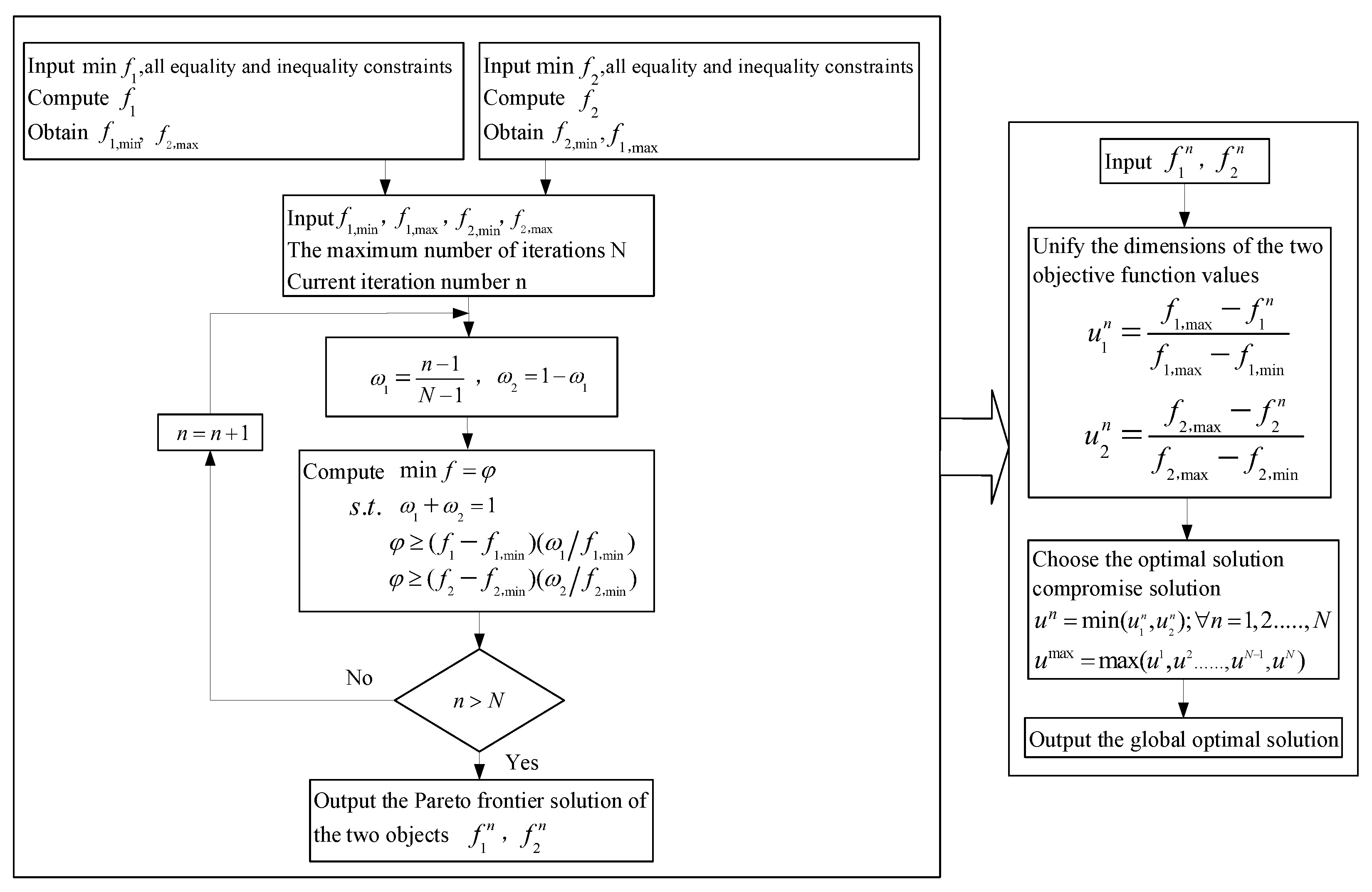
4.3. Multi-Objective Model Solving

The purchases of electricity and natural gas are the main sources of carbon emissions in this multi-objective system. Minimizing the carbon emissions requires continuously reducing the purchased amount of electricity and natural gas. However, minimizing the costs may require an appropriate increase in the purchases based on the optimal economy principle. Obviously, the two objectives cannot be achieved concurrently and are in conflict with each other. In order to realize a win–win situation without sacrificing economy or environmental protection, this paper adopts the compromise planning method illustrated in the literature [39] to solve the multi-objective model. The differences between the optimal values of the two objective functions and the criterion value are calculated when deriving the Pareto frontier solution. The optimal solution of the Pareto frontier solution is calculated by the max–min fuzzy method. The additional constraints need to be considered when solving the multi-objective functions through compromise planning [39]:

$$\{\begin{array}{c}\min f=\phi \\ {\omega }_1+{\omega }_2=1\\ \phi \ge (f_1-f_{1,\min })({\omega }_1/f_{1,\min })\\ \phi \ge (f_2-f_{2,\min })({\omega }_2/f_{2,\min })\end{array}$$

(21)

where $\phi$ is the Chebyshev distance; $f_1$ and $f_2$ are the values calculated for each iteration of objective function 1 and objective function 2, i.e., the criterion values; $f_{1,\min }$ and $f_{2,\min }$ are the minimum values of objective function 1 and objective function 2; ${\omega }_1$ and ${\omega }_2$ are the weight coefficients.

After solving the Pareto frontier solution, the two objective function values need to be normalized to unify the function dimensions. Then, the optimal solution of the Pareto frontier solution is found by using the max–min fuzzy method, which is described as follows [39]:

$${{\displaystyle u}}_k^n=\{\begin{array}{l}1,{{\displaystyle f}}_k^n\le {{\displaystyle f}}_{k,\min }\\ \frac{{{\displaystyle f}}_{k,\max }-{{\displaystyle f}}_k^n}{{{\displaystyle f}}_{k,\max }-{{\displaystyle f}}_{k,\min }},{{\displaystyle f}}_{k,\min }\le {{\displaystyle f}}_k^n\le {{\displaystyle f}}_{k,\max }\\ 0,{{\displaystyle f}}_k^n\ge {{\displaystyle f}}_{k,\max }\end{array}$$

(22)

where ${{\displaystyle u}}_k^n$ is the unit vector of the $n^{th}$ solution of the $k^{th}$ objective function; ${{\displaystyle f}}_{k,\min }$ and ${{\displaystyle f}}_{k,\max }$ are the minimum and maximum values of the Pareto solution of the objective function. The optimal solution is obtained by comparing the following equations [39]:

$$\{\begin{array}{c}{u}^n=\min (u_1^n,u_2^n);\forall n=1,2,\dots ,N\\ u^{\max }=\max (u^1,u^2,\dots ,u^{N-1},u^N)\end{array}$$

(23)

where $u^n$ is the minimum value of all solutions after unifying the values of the objective function; the maximum value among them is $u^{\max }$, which is the optimal compromise solution. The multi-objective model solving process is shown in Figure 2.

Figure 2. Multi-objective model solving flow chart.

In Figure 2, these extreme values are obtained directly by calling CPLEX. Secondly, it is necessary to initialize the iterations $n$, set the maximum number of iterations $N$, and start the iterative calculation. Thirdly, one must determine whether the maximum number of iterations is reached; if not, continue to iterate; otherwise, output the Pareto frontier solution. Finally, the optimal solution is chosen by the max–min fuzzy method.

5. Case Studies

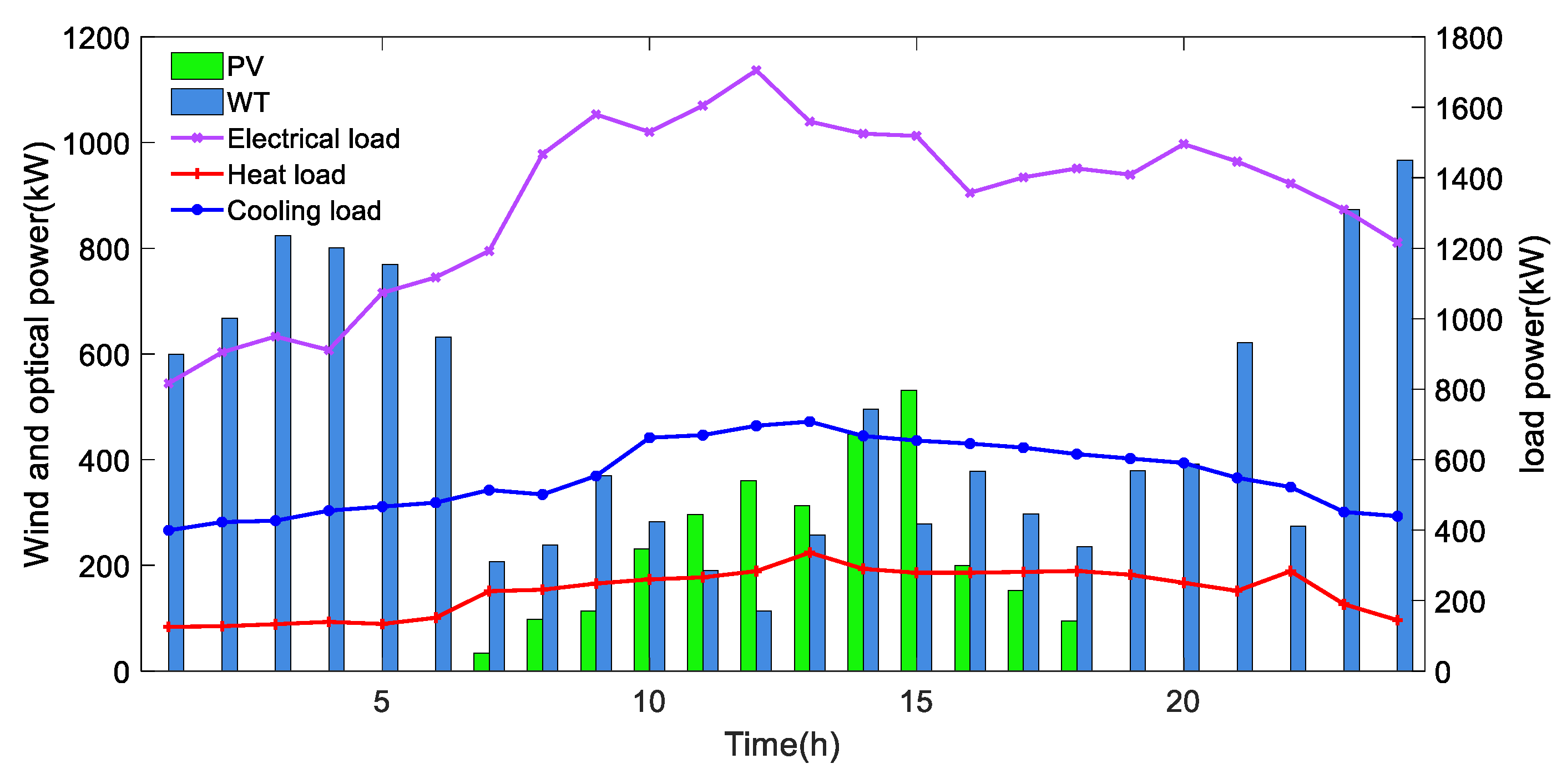
5.1. Case Condition Setting

Based on the Chongli Application Demonstration Project, the load and new energy output prediction data in the park are shown in Figure 3. It can be seen from Figure 3 that the wind power resources are sufficient at night and the photovoltaic resources are abundant during the daytime, and their complementarity allows the system to handle the load better. In addition, the electro-thermal cooling load has different demands in the time scale and space scale, and multi-energy complimentary can be realized by using a multi-energy flow coupling mechanism. A small-scale hydrogen load is set in this paper to reflect the economy of hydrogen storage, so that the system can generate income by selling the hydrogen to the outside. The electricity price and natural gas price in the time-sharing purchase from the external grid are shown in Table 2. The parameters related to each piece of equipment in the system are shown in Table 3. The efficiency parameters of the main equipment of the system are shown in Table 4. The parameters of the hydrogen storage system are taken from the literature [40]. The operating parameters of the alkaline EL are detailed in the literature [37]. The model is solved by calling CPLEX of MATLAB with a dispatch cycle of 24 h.

Figure 3. Load and new energy output.

Table 2. Time share tariffs and natural gas prices.

Energy Type	Time Period	Price
Electricity purchase price (CNY/kWh)	23:00–06:00	0.4
	07:00–09:00, 15:00–17:00, 21:00–22:00	0.8
	10:00–14:00, 18:00–20:00	1.2
Price of electricity sold (CNY/kWh)	Full day	0.35
Natural gas price (CNY/m3)	Full day	2.7

Table 3. Parameters related to each HIES device.

Equipment	Capacity (kW)	Unit Operation and Maintenance Cost (CNY/kWh)	Lifespan (Year)
CHP	1000	0.06	30
GB	1000	0.004	20
HP	600	0.007	20
EC	300	0.009	15
AC	400	0.008	15
ES	500	0.005	10
HS	600	0.002	10
CS	600	0.001	10
EL	1000	0.022	20
HFG	1000	0.042	20

Table 4. Efficiency parameters of critical equipment.

Parameters	Value	Parameters	Value
${{\displaystyle \eta }}^H$	0.75	${{\displaystyle \eta }}^{GB}$	0.93
${\eta }^{HFG}$	0.65	${{\displaystyle \eta }}^{HP}$	4
${{\displaystyle \eta }}_{CHP}^c$	0.3	${{\displaystyle \eta }}^{EC}$	3.5
${{\displaystyle \eta }}_{CHP}^h$	0.56	${{\displaystyle \eta }}^{AC}$	0.7

5.2. Analysis of Multi-Objective Robust Optimization Results

In this section, the default scenery robustness coefficient and the load robustness coefficient are described as ${{\displaystyle \Gamma }}^{wt}={{\displaystyle \Gamma }}^{pv}=0.5$, ${{\displaystyle \Gamma }}^p={{\displaystyle \Gamma }}^h={{\displaystyle \Gamma }}^c=0.05$. Other values can be set by the decision maker according to the risk preferences of the actual scheduling situation. The results of the HIES multi-objective robust optimization are shown in Figure 4, Figure 5, Figure 6 and Figure 7.

Figure 4. Electrical power optimization results.

Figure 5. Thermal power optimization results.

Figure 6. Cold power optimization results.

Figure 7. Hydrogen energy balance results.

Comparing Figure 4 and Figure 7, it can be seen that during 23:00 p.m.–6:00 a.m., the renewable energy is sufficient, the load demand is low, and the electricity has a low-valley price. The surplus electricity can be converted into hydrogen storage by the EL, which reduces the abandoned wind and solar energy to realize peak shaving and valley filling. The presence of the PV and WT allows the system to better meet the demand of the multi-load system; however, it will increase the solution uncertainty. During 10:00 a.m.–14:00 a.m. and 18:00 a.m.–20:00 a.m., the electricity purchase price is high and the cogeneration unit will cause environmental pollution, which is not conducive to the park’s low-carbon economic operation. Therefore, the HGF is operated to meet the power load demand during these hours to reduce the operational cost and the system’s carbon emissions.

As can be seen in Figure 5, the electricity prices at night are lower and the off-grid purchase carbon emissions factor is lower than that of natural gas. Therefore, the heat is mainly supplied by the HP at night to reduce the system’s operational cost and carbon emissions. When the electricity price is at its peak during the daytime, the HP output is reduced and the HIES system is mainly heated by the CHP to minimize the operational cost. Meanwhile, the excess heat is absorbed by thermal storage to avoid energy waste during the period of 23:00 p.m.–24:00 p.m.

As can be seen from Figure 6, cold energy is provided by the EC at night as the electricity price is low, and part of the cooling load demand is supplied by absorbing waste heat during the daytime. This shows that each energy source of the HIES is fully utilized and its utilization rate is improved.

In Figure 7, hydrogen energy is not only used to generate electricity for the HGF when the electricity price is high, but also supplies hydrogen to the hydrogen load. Since the income from selling hydrogen is included in the total cost of the system in this paper, the flexible application of hydrogen energy reduces the total system cost significantly.

5.3. Analysis of Multi-Objective Solutions

The multi-objective solutions considering compromise planning are shown in Figure 8 and Table 5, and the global optimal solutions yield 12,666.53 CNY and 4530.45 kg, which are the optimal system operation cost and carbon emissions.

Figure 8. Pareto frontier solution and optimal solution.

Table 5. Multi-objective Pareto solution under compromise planning.

$\mathit{n}$	${\mathit{\omega }}_1$	${\mathit{\omega }}_2$	${\mathit{u}}_1^{\mathit{n}}$	${\mathit{u}}_2^{\mathit{n}}$	${\mathit{f}}_1$ (CNY)	${\mathit{f}}_2$ (kg)
1	0	1	0.8771	1	19,641.58	4280.12
2	0.05	0.95	0.9293	0.9947	16,240.96	4368.47
3	0.1	0.9	0.9492	0.9920	14,948.75	4414.54
4	0.15	0.85	0.9612	0.9903	14,167.38	4443.29
5	0.2	0.8	0.9694	0.9891	13,634.59	4462.57
6	0.25	0.75	0.9754	0.9883	13,245.59	4475.93
7	0.3	0.7	0.9796	0.9876	12,968.09	4488.33
8	0.35	0.65	0.9821	0.9863	12,805.06	4509.61
9	0.4	0.6	0.9843	0.9851	12,666.53	4530.45
10	0.45	0.55	0.9862	0.9839	12,542.14	4550.07
11	0.5	0.5	0.9876	0.9824	12,446.63	4575.09
12	0.55	0.45	0.9889	0.9809	12,359.52	4601.64
13	0.6	0.4	0.9903	0.9793	12,273.89	4627.64
14	0.65	0.35	0.9914	0.9772	12,204.21	4662.96
15	0.7	0.3	0.9924	0.9747	12,139.22	4705.54
16	0.75	0.25	0.9935	0.9721	12,068.51	4749.29
17	0.8	0.2	0.9946	0.9690	11,996.72	4800.34
18	0.85	0.15	0.9957	0.9657	11,919.86	4857.23
19	0.9	0.1	0.9970	0.9615	11,838.28	4927.21
20	0.95	0.05	0.9984	0.9576	11,744.72	4993.36
21	1	0	0.9999	0.9511	11,694.33	5040.12

By observing the positions of the global optimal solutions in Figure 8 and Table 5, it can be seen that compromise planning is able to achieve a reasonable trade-off between the total system cost and carbon emissions and achieve a balance point between the two objectives.

In order to further verify the superiority of the multi-objective solution algorithm, all the robustness coefficients are set to 0, and then the two objectives are optimized by using the NSGA-II algorithm and the compromise planning method. The Pareto solution set resulting from these two algorithms is shown in Figure 9.

Figure 9. Distribution of Pareto solution set obtained by two optimal methods.

Compared with the NSGA II algorithm, the solution spacing in Figure 9 given by compromise planning is more uniform, and a reasonable trade-off is directly made between the cost and carbon emissions. However, its ability to approach the true Pareto front is weak.

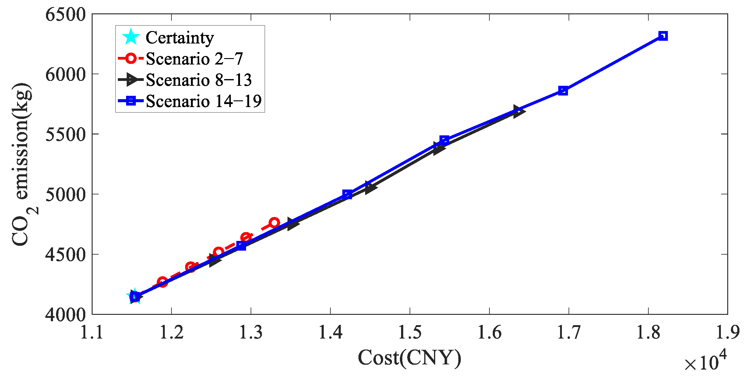
5.4. Comparison of Different Uncertainty Optimization Methods

The multi-objective deterministic optimization, multi-objective RO, and multi-objective SO are used to optimize the HIES. The robustness coefficients in the multi-objective RO are the same as in the previous section; in the deterministic optimization, the predicted values are used as data inputs; in the multi-objective SO, the source–load prediction error obeys a normal distribution, with the predicted value as the mean and 0.2 times this value as the standard deviation. The solution results of the different optimization methods are shown in Table 6.

Table 6. Results comparison of different methods.

Optimization Methods	Total System Cost (CNY)	Carbon Emission (kg)	Time (s)
Deterministic optimization	11,539.24	4146.48	35.21
Multi-objective SO	12,181.00	4357.95	390.34
Multi-objective RO	12,666.53	4530.45	36.55

As can be seen from Table 6, compared to the deterministic optimization, the total system cost and carbon emissions of the multi-objective SO increase by 5.56% and 5.10%, while those of the multi-objective RO increase by 9.77% and 9.26%. In comparison, the multi-objective RO increases the total system cost and carbon emissions by 3.99% and 3.95% over those of the multi-objective SO. This is due to the fact that the multi-objective RO’s decisions are more conservative, resulting in a relatively higher total system cost and carbon emissions, but, at the same time, it is more resilient to uncertain risks. In addition, in terms of solution time, the multi-objective SO takes the longest time when considering multiple scenarios, and the multi-objective RO is comparable to the deterministic optimization.

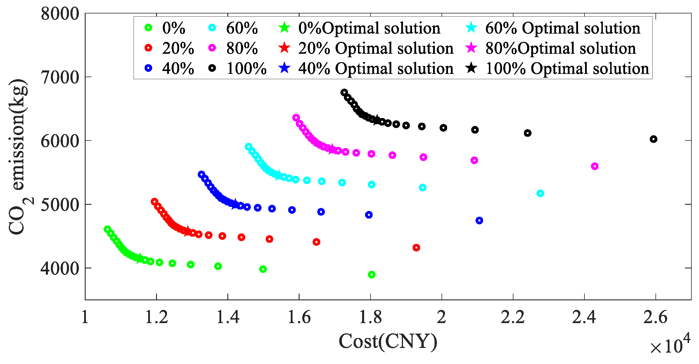
5.5. Effect of Different Robustness Factors on Multi-Objective Solutions

In this section, the source–load robustness factor is varied from 0 to 100% with 20% steps to evaluate the multi-objective solution’s effect with different robustness factors. The Pareto frontier solutions and the optimal solutions for different degrees of robustness are shown in Figure 10.

Figure 10. Pareto front solutions and optimal solutions with different robustness coefficients.

Figure 10 shows that the solutions of the two objective functions for the same system increase with the growth of the robustness factor correspondingly, while the Pareto front solution domain shrinks. The robustness coefficient’s increase leads to the conservativeness of the system’s decision making, which improves the system’s robustness but, at the same time, causes a higher total system cost and carbon emissions.

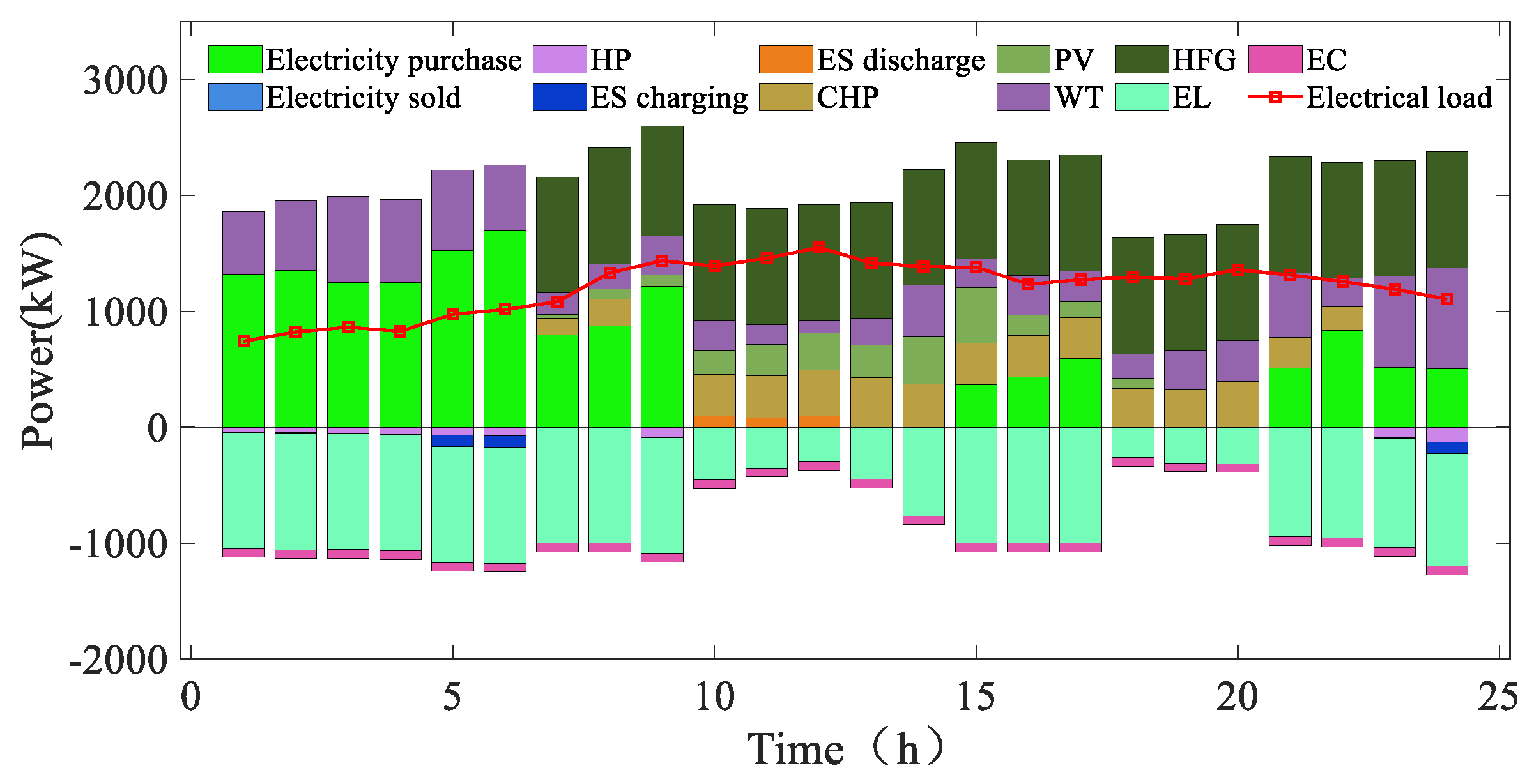
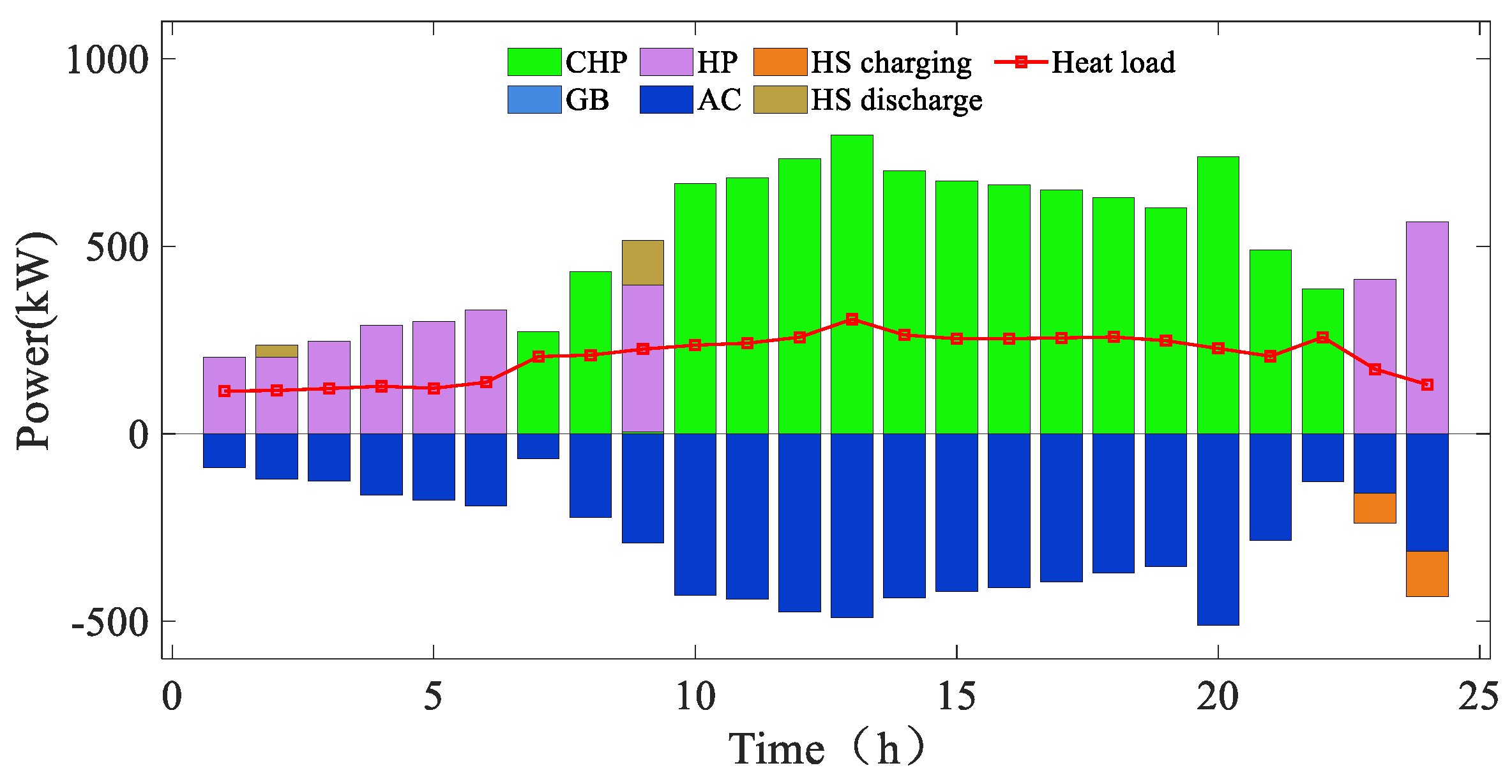
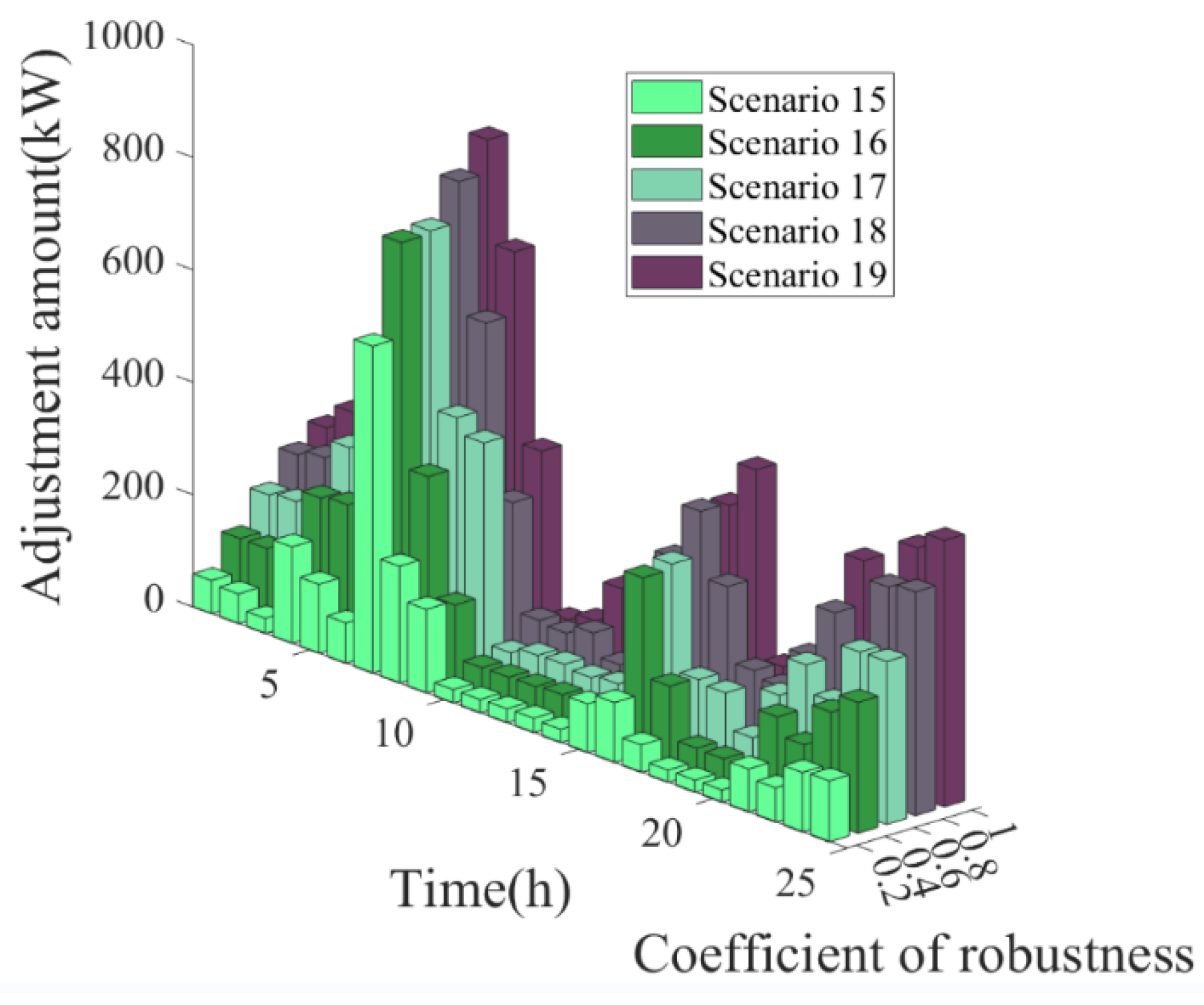
5.6. Effect of Different Robustness Factors on the Optimal Operation of the System

The five uncertainty factors are combined with 18 uncertain scenarios and 1 deterministic scenario to analyze the impact of different robustness factors, and the combination results are shown in Table 7. Among them, Scenario 1 does not consider the uncertainty, Scenarios 2 to 7 only consider the new energy output uncertainty, Scenarios 8 to 13 only consider the electric heating and cooling load uncertainty, and Scenarios 14 to 19 consider the source–load uncertainty. The operation optimization results of each scenario are shown in Table 8 and Figure 11.

Table 7. Each scenario set up by category.

Scenario	Coefficient of Robustness	Scenario	Coefficient of Robustness
1	Certainty	11	${{\displaystyle \Gamma }}^p={{\displaystyle \Gamma }}^h={{\displaystyle \Gamma }}^h=0.6$
2	${{\displaystyle \Gamma }}^{wt}={{\displaystyle \Gamma }}^{pv}=0$	12	${{\displaystyle \Gamma }}^p={{\displaystyle \Gamma }}^h={{\displaystyle \Gamma }}^h=0.8$
3	${{\displaystyle \Gamma }}^{wt}={{\displaystyle \Gamma }}^{pv}=0.2$	13	${{\displaystyle \Gamma }}^p={{\displaystyle \Gamma }}^h={{\displaystyle \Gamma }}^h=1$
4	${{\displaystyle \Gamma }}^{wt}={{\displaystyle \Gamma }}^{pv}=0.4$	14	${{\displaystyle \Gamma }}^{wt}={{\displaystyle \Gamma }}^{pv}={{\displaystyle \Gamma }}^p={{\displaystyle \Gamma }}^h={{\displaystyle \Gamma }}^c=0$
5	${{\displaystyle \Gamma }}^{wt}={{\displaystyle \Gamma }}^{pv}=0.6$	15	${{\displaystyle \Gamma }}^{wt}={{\displaystyle \Gamma }}^{pv}={{\displaystyle \Gamma }}^p={{\displaystyle \Gamma }}^h={{\displaystyle \Gamma }}^c=0.2$
6	${{\displaystyle \Gamma }}^{wt}={{\displaystyle \Gamma }}^{pv}=0.8$	16	${{\displaystyle \Gamma }}^{wt}={{\displaystyle \Gamma }}^{pv}={{\displaystyle \Gamma }}^p={{\displaystyle \Gamma }}^h={{\displaystyle \Gamma }}^c=0.4$
7	${{\displaystyle \Gamma }}^{wt}={{\displaystyle \Gamma }}^{pv}=1$	17	${{\displaystyle \Gamma }}^{wt}={{\displaystyle \Gamma }}^{pv}={{\displaystyle \Gamma }}^p={{\displaystyle \Gamma }}^h={{\displaystyle \Gamma }}^c=0.6$
8	${{\displaystyle \Gamma }}^p={{\displaystyle \Gamma }}^h={{\displaystyle \Gamma }}^h=0$	18	${{\displaystyle \Gamma }}^{wt}={{\displaystyle \Gamma }}^{pv}={{\displaystyle \Gamma }}^p={{\displaystyle \Gamma }}^h={{\displaystyle \Gamma }}^c=0.8$
9	${{\displaystyle \Gamma }}^p={{\displaystyle \Gamma }}^h={{\displaystyle \Gamma }}^h=0.2$	19	${{\displaystyle \Gamma }}^{wt}={{\displaystyle \Gamma }}^{pv}={{\displaystyle \Gamma }}^p={{\displaystyle \Gamma }}^h={{\displaystyle \Gamma }}^c=1$
10	${{\displaystyle \Gamma }}^p={{\displaystyle \Gamma }}^h={{\displaystyle \Gamma }}^h=0.4$

Table 8. Scheduling results for various scenarios.

Scenario	Total System Cost (CNY)	Carbon Emissions (kg)	Scenario	Total System Cost (CNY)	Carbon Emissions (kg)
1	11,539.24	4146.48	11	14,492.35	5053.86
2	11,539.24	4146.48	12	15,350.51	5379.55
3	11,887.88	4269.00	13	16,357.64	5687.24
4	12,241.56	4392.78	14	11,539.24	4146.48
5	12,593.44	4516.13	15	12,876.22	4571.42
6	12,937.43	4637.57	16	14,209.94	4997.08
7	13,294.34	4762.21	17	15,433.65	5449.32
8	11,539.24	4146.48	18	16,928.91	5860.91
9	12,527.69	4448.81	19	18,186.84	6317.29
10	13,512.07	4751.44

Figure 11. Comparison of different scenarios.

Comparing Scenarios 1, 2, 8, and 14 in Table 8, when the robustness coefficients of all four scenarios are zero, the total system cost and carbon emissions are the same, and the model degenerates to become deterministic. This verifies the generality and correctness of the multi-objective robust optimization model.

Scenarios 2 to 7, Scenarios 8 to 13, and Scenarios 14 to 19 show that the total system cost and carbon emissions increase with the robustness factor. This indicates that the uncertainty set increases with the robustness factor accordingly, leading to more conservative decisions.

Comparing Scenarios 2–7 with Scenarios 8–13 reveals that the latter have a greater increase in the total system cost and carbon emissions than the former, with the same robustness factor growth. This illustrates that the energy production can be transferred directly to the load side with lower losses and the load side uncertainty impacts the HIES operation greatly.

By comparing Scenarios 7, 13, and 19, it can be seen that Scenario 19 has the largest operating cost and carbon emissions when the robustness coefficient of the three scenarios is 1, which is the most robust case. This shows that the source–load uncertainty, when considered comprehensively, will influence the system’s operation significantly.

Therefore, decision makers can adjust the robustness coefficient individually in the actual scheduling process according to the amount of acceptable risk, so as to make reasonable decisions.

Figure 12 and Table 9 show the unit power adjustments of each time period and the total values with different robustness coefficients for Scenarios 15–19 in Table 7. The total adjustment refers to the sum of the power purchased, the CHP power, and the GB power increased by the uncertainty of the source charge over the deterministic model for 24 h.

Figure 12. Unit output adjustment with different robustness factors.

Table 9. Total adjustment of unit output with different robustness factors.

Scenario	15	16	17	18	19
Adjusted total amount (kW)	2124	3656	5067	6684	7869

The system output increases to different degrees at each time in Figure 12. This indicates that the difference between the load power (electric, thermal, and cold) and the source output (WT and PV) fluctuates upwards. Therefore, the power purchase, CHP, and GB all need to increase in output in order to maintain the energy balance. In addition, Table 9 and Figure 12 reveal that the total power increases to 2124 kW, 3656 kW, 5067 kW, 6684 kW, and 7869 kW when the robustness coefficients are 0.2, 0.4, 0.6, 0.8, and 1, respectively, which indicates that the larger the robustness coefficient, the greater the system uncertainty, the more conservative the decisions, and the larger the total power.

6. Conclusions and Future Work

6.1. Conclusions

An integrated energy system containing hydrogen storage is proposed based on the Chongli Large-Scale Wind–Solar Complementary Coupled Hydrogen Production System Application Demonstration Project. Considering the source–load uncertainty of the system, multi-objective optimization is combined with RO to establish the HIES multi-objective robust optimization model, and the proposed method is verified by practical data. The results show the following.

(1)

The HIES multi-objective robust optimization model can reduce the wind and solar abandonment significantly, decrease the purchased amount of electricity and gas in the park, restrain the system’s operational cost and carbon emissions, and improve the utilization rate of each energy source effectively.

(2)

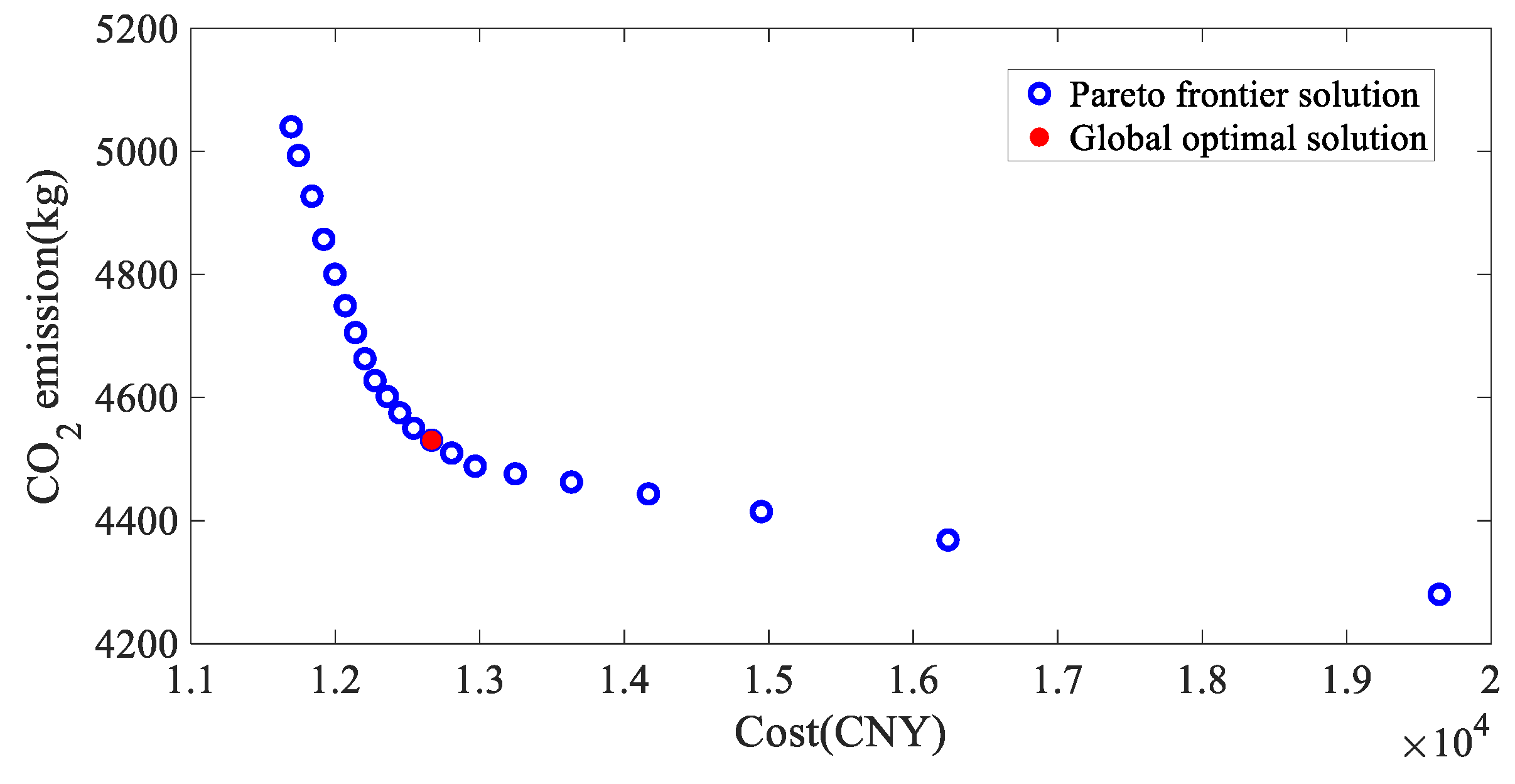
The compromise planning method achieves a reasonable balance between the two objectives of total system cost and carbon emissions, to realize a win–win situation between both objectives, where their optimal solutions are 12,666.53 CNY and 4530.45 kg. Compared with NSGA-II, compromise programming has a more uniform solution set but is less capable of approaching the true Pareto front, which is one of its limitations.

(3)

Compared with the multi-objective SO, the multi-objective RO has a faster solution speed and better robustness. However, its total system cost and carbon emissions increase by 3.99% and 3.95%, which is a minor limitation. In addition, the decision maker can adjust the robustness coefficients in real scheduling situations to reduce the decision-making conservativeness and overcome the strong conservativeness of the traditional RO.

6.2. Future Work

There are still some considerations for further study.

The HIES multi-objective robust optimization model developed in this paper promotes the development of a low-carbon economy. However, RO is used to deal with the uncertainty of the HIES, with high solving efficiency, but it may also have resulted in overly conservative decision making. Therefore, DRO will be introduced to balance the robustness and economy in the future.

References

- Liu, D.; Luo, Z.; Qin, J.; Wang, H.; Wang, G.; Li, Z.; Zhao, W.; Shen, X. Low-carbon dispatch of multi-district integrated energy systems considering carbon emission trading and green certificate trading. Renew. Energy 2023, 218, 119312. [Google Scholar] [CrossRef]
- Wei, G.; Yan, M.; Yao, W.; Guo, J.; Ai, X.; Fang, J.; Wen, J. Decentralized computation method for robust operation of multi-area joint regional-district integrated energy systems with uncertain wind power. Appl. Energy 2021, 298, 117280. [Google Scholar]
- Li, H.; Qin, B.; Jiang, Y.; Zhao, Y.; Shi, W. Data-driven optimal scheduling for underground space based integrated hydrogen energy system. IET Renew. Power Gener. 2022, 16, 2521–2531. [Google Scholar] [CrossRef]
- Fang, X.; Dong, W.; Wang, Y.; Yang, Q. Multi-stage and multi-timescale optimal energy management for hydrogen-based integrated energy systems. Energy 2023, 286, 129576. [Google Scholar] [CrossRef]
- Ahmadi, S.; Sadeghi, D.; Marzband, M.; Abusorrah, A.; Sedraoui, K. Decentralized bi-level stochastic optimization approach for multi-agent multi-energy networked micro-grids with multi-energy storage technologies. Energy 2022, 245, 123223. [Google Scholar] [CrossRef]
- Dong, X.; Wu, J.; Xu, Z.; Liu, K.; Guan, X. Optimal coordination of hydrogen-based integrated energy systems with combination of hydrogen and water storage. Appl. Energy 2022, 308, 118274. [Google Scholar] [CrossRef]
- Zhong, Z.; Huang, D.; Hu, K.; Ai, X.; Fang, J. Real-time Optimal Operation of Microgrid with Power-to-hydrogen. In Proceedings of the 2020 IEEE Sustainable Power and Energy Conference (iSPEC), Chengdu, China, 23–25 November 2020; pp. 2275–2280. [Google Scholar]
- Pu, Y.; Li, Q.; Zou, X.; Li, R.; Li, L.; Chen, W.; Liu, H. Optimal sizing for an integrated energy system considering degradation and seasonal hydrogen storage. Appl. Energy 2021, 302, 117542. [Google Scholar] [CrossRef]
- Li, J.; Lin, J.; Song, Y.; Xing, X.; Fu, C. Operation optimization of Power to Hydrogen and Heat (P2HH) in ADN Coordinated with the District Heating Network. IEEE Trans. Sustain. Energy 2019, 10, 1672–1683. [Google Scholar] [CrossRef]
- Wang, Y.; Song, M.; Jia, M.; Li, B.; Fei, H.; Zhang, Y.; Wang, X. Multi-objective distributionally robust optimization for hydrogen-involved total renewable energy CCHP planning under source-load uncertainties. Appl. Energy 2023, 342, 121212. [Google Scholar] [CrossRef]
- Fang, R. Multi-objective optimized operation of integrated energy system with hydrogen storage. Int. J. Hydrog. Energy 2019, 44, 29409–29417. [Google Scholar]
- Zhou, J.; Wu, Y.; Zhong, Z.; Xu, C.; Ke, Y.; Gao, J. Modeling and configuration optimization of the natural gas-wind-photovoltaic-hydrogen integrated energy system: A novel deviation satisfaction strategy. Energy Convers. Manag. 2021, 243, 114340. [Google Scholar] [CrossRef]
- Shi, M.; Wang, W.; Han, Y.; Huang, Y. Research on comprehensive benefit of hydrogen storage in microgrid system. Renew. Energy 2022, 194, 621–635. [Google Scholar] [CrossRef]
- Song, Y.; Mu, H.; Li, N.; Wang, H. Multi-objective optimization of large-scale grid-connected photovoltaic-hydrogen-natural gas integrated energy power station based on carbon emissions priority. Int. J. Hydrog. Energy 2023, 48, 4087–4103. [Google Scholar] [CrossRef]
- Yang, X.; Leng, Z.; Xu, S.; Yang, C.; Yang, L.; Liu, K.; Song, Y.; Zhang, L. Multi-objective optimal scheduling for CCHP microgrids considering peak-load reduction by augmented ε-constraint method. Renew. Energy 2021, 172, 408–423. [Google Scholar] [CrossRef]
- Kamarposhti, M.; Colak, I.; Shokouhandeh, H.; Iwendi, C.; Padmanaban, S.; Band, S. Optimum operation management of microgrids with cost and environment pollution reduction approach considering uncertainty using Multi-objective NSGAII algorithm. IET Renew. Power Gener. 2022, 1–13. [Google Scholar] [CrossRef]
- Huang, C.; Bai, Y.; Yan, Y.; Zhang, Q.; Zhang, N.; Wang, W. Multi-objective co-optimization of design and operation in an independent solar-based distributed energy system using genetic algorithm. Energy Convers. Manag. 2022, 271, 116283. [Google Scholar] [CrossRef]
- Parvin, M.; Yousefi, H.; Noorollahi, Y. Techno-economic optimization of a renewable micro grid using multi-objective particle swarm optimization algorithm. Energy Convers. Manag. 2023, 277, 116639. [Google Scholar] [CrossRef]
- Kuang, H.; Su, F.; Chang, Y.; Wang, K.; He, Z. Reactive power optimization for distribution network system with wind power based on improved multi-objective particle swarm optimization algorithm. Electr. Power Syst. Res. 2022, 213, 108731. [Google Scholar]
- Maharjan, K.; Zhang, J.; Cho, H.; Chen, Y. Distributed Energy Systems: Multi-Objective Design Optimization Based on Life Cycle Environmental and Economic Impacts. Energies 2023, 16, 7312. [Google Scholar] [CrossRef]
- Liu, Z.; Cui, Y.; Wang, J.; Chang, Y.; Agbodjan, Y.S.; Yang, Y. Multi-objective optimization of multi-energy complementary integrated energy systems considering load prediction and renewable energy production uncertainties. Energy 2022, 254, 124399. [Google Scholar] [CrossRef]
- Wang, M.; Yu, H.; Jing, R.; Liu, H.; Chen, P.; Li, C. Combined multi-objective optimization and robustness analysis framework for building integrated energy system under uncertainty. Energy Convers. Manag. 2020, 208, 112589. [Google Scholar] [CrossRef]
- Ju, L.; Tan, Q.; Lin, H.; Mei, S.; Li, N.; Lu, Y.; Wang, Y. A two-stage optimal coordinated scheduling strategy for micro energy grid integrating intermittent renewable energy sources considering multi-energy flexible conversion. Energy 2020, 196, 117078. [Google Scholar] [CrossRef]
- Kheirkhah, A.; Meschini Almeida, C.; Kagan, N.; Leite, J. Optimal Probabilistic Allocation of Photovoltaic Distributed Generation: Proposing a Scenario-Based Stochastic Programming Model. Energies 2023, 16, 7261. [Google Scholar] [CrossRef]
- Qiu, Y.; Li, Q.; Huang, L.; Sun, C.; Wang, T.; Chen, W. Adaptive uncertainty sets-based two-stage robust optimization for economic dispatch of microgrid with demand response. IET Renew. Power Gener. 2020, 14, 3608–3615. [Google Scholar] [CrossRef]
- Ren, T.; Li, R.; Li, X. Bi-level multi-objective robust optimization for performance improvements in integrated energy system with solar fuel production. Renew. Energy 2023, 219, 119499. [Google Scholar] [CrossRef]
- Mohammadi, M.; Noorollahi, Y.; Mohammadi-ivatloo, B. Fuzzy-based scheduling of wind integrated multi-energy systems under multiple uncertainties. Sustain. Energy Technol. Assess. 2020, 37, 100602. [Google Scholar] [CrossRef]
- Su, Y.; Zhou, Y.; Tan, M. An interval optimization strategy of household multi-energy system considering tolerance degree and integrated demand response. Appl. Energy 2020, 260, 114144. [Google Scholar] [CrossRef]
- Thang, V.; Thanhtung, H.; Li, Q.; Zhang, Y. Stochastic optimization in multi-energy hub system operation considering solar energy resource and demand response. Int. J. Electr. Power Energy Syst. 2022, 141, 108132. [Google Scholar] [CrossRef]
- Wei, X.; Sun, Y.; Zhou, B.; Zhang, X.; Wang, G.; Qiu, J. Carbon emission flow oriented multitasking multi-objective optimization of electricity-hydrogen integrated energy system. IET Renew. Power Gener. 2022, 16, 1474–1489. [Google Scholar] [CrossRef]
- Mansour-Saatloo, A.; Agabalaye-Rahvar, M.; Mirzaei, M.; Mohammadi-Ivatloo, B.; Abapour, M.; Zare, K. Robust scheduling of hydrogen based smart micro energy hub with integrated demand response. J. Clean. Prod. 2020, 267, 122041. [Google Scholar] [CrossRef]
- Yang, J.; Su, C. Robust optimization of microgrid based on renewable distributed power generation and load demand uncertainty. Energy 2021, 223, 120043. [Google Scholar] [CrossRef]
- Cai, P.; Mi, Y.; Ma, S.; Li, H.; Li, D.; Wang, P. Hierarchical game for integrated energy system and electricity-hydrogen hybrid charging station under distributionally robust optimization. Energy 2023, 283, 128471. [Google Scholar] [CrossRef]
- Yan, R.; Lu, Z.; Wang, J.; Chen, H.; Wang, J.; Yang, Y.; Huang, D. Stochastic multi-scenario optimization for a hybrid combined cooling, heating and power system considering multi-criteria. Energy Convers. Manag. 2021, 233, 113911. [Google Scholar] [CrossRef]
- Lian, Y.; Li, Y.; Zhao, Y.; Yu, C.; Zhao, T.; Wu, L. Robust multi-objective optimization for islanded data center microgrid operations. Appl. Energy 2023, 330, 120344. [Google Scholar] [CrossRef]
- Yang, Y.; Wu, W. A Distributionally Robust Optimization Model for Real-Time Power Dispatch in Distribution Networks. IEEE Trans. Smart Grid 2019, 10, 3743–3752. [Google Scholar] [CrossRef]
- Li, H.; Xue, Y.; Dai, T.; Chang, X.; Pan, Z.; Sun, H. Collaborative Optimal Dispatch of Electricity—Hydrogen Coupling System in Chemical Industry Park Considering Hydrogen Load Response. Adv. Eng. Sci. 2023, 55, 93–100. [Google Scholar]
- Rahimiyan, M.; Baringo, L. Strategic bidding for a virtual power plant in the day-ahead and real-time markets: A price-taker robust optimization approach. IEEE Trans. Power Syst. 2016, 31, 2676–2687. [Google Scholar] [CrossRef]
- Pei, M.; Yue, Z.; Tong, N.; As’ad, A.; Kittisak, J. Optimal emission management of photovoltaic and wind generation based energy hub system using compromise programming. J. Clean. Prod. 2020, 281, 124333. [Google Scholar]
- Li, X.; Yang, Y.X. Optimization Dispatching for Joint Operation of Hydrogen Storage-wind Power and Cascade Hydropower Station Based on Bidirectional Electricity Price Compensation. Power Syst. Technol. 2020, 44, 3297–3306. [Google Scholar]
Disclaimer/Publisher’s Note: The statements, opinions and data contained in all publications are solely those of the individual author(s) and contributor(s) and not of MDPI and/or the editor(s). MDPI and/or the editor(s) disclaim responsibility for any injury to people or property resulting from any ideas, methods, instructions or products referred to in the content. |
© 2024 by the authors. Licensee MDPI, Basel, Switzerland. This article is an open access article distributed under the terms and conditions of the Creative Commons Attribution (CC BY) license (https://creativecommons.org/licenses/by/4.0/).