Abstract
Photovoltaic (PV) power generation forecasting is an important research topic, aiming to mitigate variability caused by weather conditions and improve power generation planning. Climate factors, including solar irradiance, temperature, and cloud cover, influence the energy conversion achieved by PV systems. Long-term weather forecasting improves PV power generation planning, while short-term forecasting enhances control methods, such as managing ramp rates. The stochastic nature of weather variables poses a challenge for linear regression methods. Consequently, advanced, state-of-the-art machine learning (ML) approaches capable of handling non-linear data, such as long short-term memory (LSTM), have emerged. This paper introduces the implementation of a multivariate machine learning model to forecast PV power generation, considering multiple weather variables. A deep learning solution was implemented to analyze weather variables in a short time horizon. Utilizing a hidden Markov model for data preprocessing, an LSTM model was trained using the Alice Spring dataset provided by DKA Solar Center. The proposed workflow demonstrated superior performance compared to the results obtained by state-of-the-art methods, including support vector machine, radiation classification coordinate with LSTM (RCC-LSTM), and ESNCNN specifically concerning the proposed multi-input single-output LSTM model. This improvement is attributed to incorporating input features such as active power, temperature, humidity, horizontal and diffuse irradiance, and wind direction, with active power serving as the output variable. The proposed workflow achieved a mean square error (MSE) of , a root mean square error (RMSE) of , and a mean absolute error (MAE) of .
1. Introduction
The constant increase in electric energy use around the world poses an important challenge to electric power generation []. Transitions to renewable energy are occurring because non-renewable energy is not viable in the long term due to social and environmental concerns and conventional fuel supply issues. Different energy sources would be needed to cover fluctuations from the sun or the wind and guarantee a quality service. For example, storage technologies would provide alternative supply during energy deficiencies due to cloud cover or at night.
Solar energy is the most used renewable energy source in the world, having generated 855.7 TWh by the end of 2020 []. PV systems are the main technologies based on solar energy resources [,]. The energy transformations achieved by PV panels are affected by manufacturing factors associated with materials, maintenance, cleaning, dimensions [], and climate factors, grouped into atmospheric parameters, solar irradiance, and geographic characteristics. Table 1 presents some weather variables that affect power generation from PV systems []. Irradiance has the highest correlation with the power output, as proven in previous works and later in this paper, with a correlation coefficient of 0.96. Irradiance and other weather variables exhibit stochastic behavior, which makes classic statistical methods ineffective in predicting their behavior.

Table 1.
Classified weather variables.
Weather variables can be analyzed at different time horizons, which can be grouped into very short-term (<30 min), short-term (between 30 min and 6 h), and long-term time horizons (between 4 and 6 h) []. Another option is to group variables as intra-hour (15 min to 2 h), intra-day (1 to 6 h), and day-ahead (1 day to 3 days) []. Each group has different sources of information; for example, the long-term horizon uses satellite images, and the short term uses sky images. Prediction in the medium or long term has a high error rate. On the other hand, very short-term predictions have better accuracy and are used in power generation planning [] or applications such as ramp rate in PV power [].
There are diverse approaches to predicting environmental characteristics, such as time horizon, machine learning, and deep learning methods and those that estimate variables. For example, when grouping by method, the proposed groups are statistical models, cloud image models, numeric models, and hybrid models. Statistical models work with historical data to predict the subsequent values, and these models can be sub-grouped into statistical or linear models and artificial intelligence or non-linear models. Some examples of linear models are stationary analysis, autoregressive integrated moving average (ARIMA), multiple regressions, and exponential smoothing. Nonlinear models include fuzzy inferences, genetic algorithms, neural networks, and machine learning methods []. These linear and non-linear models are used in very short-term or intra-hour groupings. Artificial intelligence methods are well-suited for managing diverse problems. For example, neural networks are a great tool for solar irradiance prediction, and the most popular method for this prediction is multilayer perceptron (MLP) []. Distinguishing spurious results from actual cloud dynamics is an important problem. Dips from actual cloud dynamics can be identified as outliers and eliminated in the preprocessing stage. However, an initial model outlining common behavior for PV power generation could be used as a first step, with any relevant dips modeled at a subsequent stage. The initial baseline modeling might depend on the dataset used.
1.1. Related Works
Some relevant works for predicting power output in PV systems address the issue of discontinuous or sudden fluctuation in power generation due to factors such as temperature, wind velocity, cloud cover, and other weather variables []. This analysis and prediction use a short time horizon (0.5 to 6 h), and prediction is achieved with machine learning methods, particularly with support vector machine (SVM). Another paper compared multiple linear regression (MLR), decision tree (DTR), and k-nearest neighbor (KNN); the author concluded that KNN is the best machine learning method because it had more accurate predictions compared to the other models [].
In another paper, three linear methods were compared on their ability to predict PV power output: autoregressive (AR), LM model, and exogenous input (ARX). All performed well in stable conditions but yielded inaccurate results under unexpected fluctuations; the ARX model produced better results []. Another author used convolutional neural network (CNN) and long short-term memory (LSTM) to create a robust deep spatiotemporal model named convolutional LSTM (ConvLSTM) to work in multiples regions or PV systems that are separated from each other []. ConvLSTM was compared to the ARMA model and fully connected LSTM (FC-LSMT); ConvLSTM produced better results.
Recurrent neural networks (RNNs) and LSTM architectures have been used to create a new framework for sequence learning named Evolino []. The Evolino framework was probed with a Mackey–Glass time series prediction. In order to perform power prediction, a path with three stages was proposed: data preprocessing to treat missing values, data normalization, and parameter initialization []. In the second stage, a radiation coordinate classification method was employed based on the correlation between different features at different times, typically in the time window 8:30–17:30. This classification method categorizes data points into specific radiation coordinates, capturing variations in solar radiation levels. Finally, the preprocessed and classified data were input into an LSTM model for power forecasting; the model was assessed using the benchmark dataset DKASC []. The evaluation metrics RMSE and mean absolute percentage error (MAPE) were reported to evaluate the accuracy of the model.
One study proposed an examination of the impact of the configuration and selection of hyperparameters in an LSTM architecture. The objective was to establish the different contributions of the LSTM configuration, input, forgetting, and output gates in forecasting applications []. Another work proposed a feature extraction method based on sentiment analysis. Concatenated time series information of prices and other variables were used as input in prediction models, including random forest, LSTM, and multilayer perceptron [].
Another proposed approach focused on preprocessing the data to remove abnormalities by performing data normalization []. Subsequently, the ESN-CNN model is trained, combining the echo state network (ESN) and convolutional neural network (CNN) to extract spatial features from the data. This hybrid model aims to leverage the capabilities of both ESN and CNN for improved performance. Finally, the model is assessed using the DKASC dataset [], and metrics such as RMSE and MAPE are reported to evaluate its accuracy. Table 2 summarizes the related works and highlights their advantages and disadvantages.

Table 2.
Related work summary.
1.2. Contributions
The main contributions of this paper are:
- A robust and precise workflow to power prediction is presented, leveraging hidden Markov models to effectively identify outliers within the raw weather data. Moreover, a deep learning LSTM architecture is designed to enhance PV prediction performance, surpassing the results reported in [,,].
- PV prediction is performed at short time horizons (five minutes ahead) with time steps of five minutes using the ambient weather dataset on Puerto Rico. The Caribbean location introduces challenges, as historically, weather predictions have been unreliable due to the high variability of winds and the complicated dynamics of the heat patterns throughout the day from both sea and land.
This paper presents an implementation of a machine learning model to predict the power output of a PV system consisting of two subprocesses: the preprocessing stage and the trained model for power prediction. The initial preprocessing involves the application of a hidden Markov model (HMM) to automatically detect and eliminate outliers. Subsequently, the LSTM model is trained to predict the common behavior of power generation, establishing a baseline model as the initial step toward future work specifically addressing outlier prediction in the context of Puerto Rico. The two variations of the LSTM are presented: one uses a single input to obtain a single output (SISO), and the other uses multiple inputs to obtain a single output (MISO). The prediction horizon was set at a short time (five minutes ahead) to assess the effectiveness of HMM outlier detection and elimination. This specific time horizon captures the dynamic behavior of clouds and their impact on PV systems.
1.3. Outline
To outline the proposed method, this paper is separated into six sections. The introduction sets the stage by presenting the motivation, context, related works on PV systems and weather forecasting, and the primary contributions of this study. The proposed workflow details the stages for constructing the proposed machine learning model, with each step described in subsections. The third section describes the two datasets employed. The results outlined in section four showcase outcomes across six experiments and employ metrics for comparison with state-of-the-art solutions. The fifth section presents a discussion and interprets the results in the context of enhancing PV systems. Lastly, the sixth section provides a concise summary and conclusions, encapsulating the essential findings and contributions of this paper.
2. Proposed Workflow
Power output prediction in PV systems needs multiple steps to prepare the data, train the model, and compute the results. Figure 1 presents a workflow used to build a machine learning model.
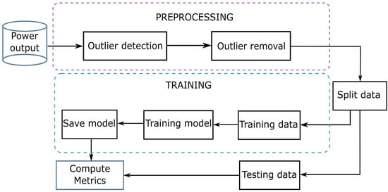
Figure 1.
Workflow used to build a machine learning model.
In addition, Table 3 presents a detailed summary of the variables.

Table 3.
Notation used in the article.
2.1. Input Variables
The first step in the workflow is related to the dataset and variables used. The dataset has the following variables: active energy delivered/received, active power, current phase average, wind speed, temperature, humidity, horizontal and diffuse irradiance, wind direction, weather daily rainfall, radiation global tilted, and radiation diffuse tilted.
The input data were normalized using min–max scaling; this process transforms the amplitude of each variable to values between 0 and 1. Normalization allows the comparison of different variables in the same space while simplifying amplitude information. To perform the model generalization and avoid overfitting, the NaN values are removed from the data and replaced by the mean values from a neighborhood.
2.2. Outlier Detection and Removal
The power output and other variables typically have outliers generated by cloud cover. In [], the authors mention that shadows are the most negative environmental factor for PV power systems.
In the outlier detection phase, the difference between points in the signal is computed as follows.
where is the magnitude of feature in the time . A large value represents an unusual value or outlier, and a small value represents a normal value. The Gaussian HMM classifies each point using the computed feature Diff. Three classes configured in the HMM model were: outlier, inlier, and constant.
HMM is a process involving the evolution of hidden states over time. In other words, it describes the transitions between hidden states. These states are associated with observations corrupted by noise. If the state variables are and the corresponding observation variables are , an HMM can be parametrized by an initial distribution , transition probabilities , and observation probabilities []. The joint distribution of a length is factorized as:
where represents a particular assignment of hidden state and represents an observation variable []. The hidden states used in this implementation are 0 and 2 for inliers or normal values and 1 for outliers.
According to the Gaussian HMM approach, the prior probability is obtained from the probability distribution function (PDF). The PDF provides approximations of Gaussian densities [,], which are obtained by:
where and are estimated from each observation.
The output from the outlier detection step is a classification of measures; this classification is used in the outlier removal step to smooth the measures with higher differences. Finally, the output of the outlier removal step is the time series signal without outliers. The best performance is obtained when three classes are configured to classify the measures. These classes can be described as follows: zero or minimal differences (indicated in Figure 2 by blue dots), small differences (orange dots), and higher differences (green dots). For example, in Figure 2, the power output in one day is presented, the signal has outliers, and the outlier detection step classifies the points as outliers with green dots or normal values with orange and blue dots.
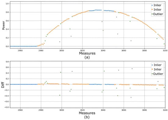
Figure 2.
Time series signal before removal of outliers. (a) Power generation vs. measures are classified as outliers with class label 1 (green dots) or normal values with class labels 0 and 2 (blue and orange dots) for HMM. (b) Diff variable vs. measures classified from HMM.
Figure 3 shows the signal output of the outlier removal step, where all outliers have been eliminated. It is observed that the difference in amplitude is less than 0.06 due to imperfections in the signal.
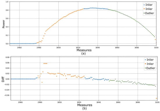
Figure 3.
Timeseries signal after the outlier removal step. (a) Power generation vs. measures are classified as outliers with class label 1 (green dots) or normal values with class labels 0 and 2 (blue and orange dots) for HMM. (b) Diff variable vs. measures classified from HMM.
2.3. Split Data
The available measurements are divided into three groups: testing, training, and validation. The percentage is chosen heuristically as follows: the testing group has 30% of the measurements, the training group has 40%, and the validation group has 30%. Each of these groups is used in different steps in the next stages.
2.4. Training Data
Since statistical methods are ineffective in the prediction of irradiance and other weather variables [], artificial intelligence methods have gained acceptance and are well-suited for PV power prediction. For example, neural networks are a great tool for solar irradiance prediction, and the most popular method for this prediction is multilayer perceptron (MLP) []. Deep learning is a subcategory of artificial intelligence where methods are used to resolve complex non-linear problems []. Some of the main methods are: convolutional neural network (CNN), support vector machine (SVN), long short-term memory (LSTM), and recurrent neural networks (RNN). LSTM is typically used for time series variables such as irradiance and other weather features.
Training data are represented by , where is the position of the measurement, and , where is the number of measures in the training data. Using generates two vectors, and , where:
Equations (4) and (5) generate two vectors with length n − 1; both vectors fit the model in the training block. The vector represents the present measure, and the vector represents the future desired value. Both vectors are given after the application of the outlier detection and removal steps using HMM.
2.5. Testing Data
The testing data have two vectors, and , computed from Equations (4) and (5), and n is the number of measures in the testing data. Both vectors are used to test the built model in the training block. The vector represents the present measure and input to the model; the output model is the predicted vector . The vector is used to compute metrics and is explained in Section 2.7 (Metrics).
2.6. Training Model
The power prediction methods applied to PV systems have been extensively addressed in [,,,,]. In recent years, deep learning methods, particularly those utilizing long short-term memory (LSTM) networks, have gained significant attention for time series prediction problems [], outperforming traditional machine learning techniques in terms of MSE and RMSE []. This paper presents an approach based on SISO and MISO LSTM models, wherein a hidden Markov model removes outliers for power prediction.
2.6.1. Long Short-Term Memory (LSTM)
LSTM is a deep learning method used for time series prediction. A key feature of LSTM is the possibility of protecting the memory cells using sigmoid gates []. With this, the LSTM method can update the output based on previous outputs and present input data []. Figure 4 presents the cell components in LSTM.
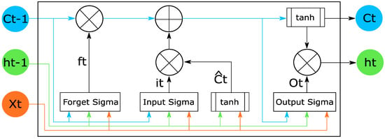
Figure 4.
LSTM cell components.
Each LSTM cell receives the previous state , the previous hidden state , and the actual measure . Forget gate, input gate, and output gate use the sigmoid function to protect the memory cell [].
For a single LSTM cell, as presented in Figure 4, it is possible to calculate the values using the equations in (6).
where is the sigmoid function used as activation function, and is the dot operator or dot product operation. Finally, and are configuration parameters [].
The LSTM implemented uses and initial values in zeros. The output is taken as .
2.6.2. Implementation
The proposed SISO and MISO LSTM models were implemented using TensorFlow version 2.11.0 []. For the SISO LSTM model, the network hyperparameters were configured with four neurons in the hidden layer and trained for ten epochs, with a batch size of 1. The learning rate was set to , the optimizer used was Adam, and the optimization metric was mean squared error (MSE).
The MISO LSTM model was configured with three hidden layers, followed by a dense operation, and trained for 200 epochs. The optimizer used was Adam, and the loss function employed was MSE. The batch size was determined by grouping the following features: active power, temperature, humidity, horizontal irradiance, diffuse irradiance, and wind direction. These features were set as the input for the MISO LSTM model to perform power prediction as the target.
2.7. Metrics
In order to evaluate the performance of the proposed MISO and SISO LSTM models, the following metrics were employed: mean squared error (MSE), root mean squared error (RMSE), and mean absolute error (MAE). These models were tested using the benchmark dataset DKA Solar and Ambient Weather dataset.
3. Dataset Description
In order to evaluate the proposed SISO and MISO LSTM models, experiments were conducted using two distinct benchmark datasets: DKA Solar and Ambient Weather. The details of each dataset are described as follows:
- DKA Solar []: This online hub provides a platform for sharing variable weather measurements obtained from PV farms located in Australia. The dataset used to evaluate the proposed models spans from 2013 to 2020, with 1,281,324 measurements taken every five minutes. The first 12,950 dataset values were not used because there are no active power values; however, the number of samples is high, with 1,268,374 measurements. In addition, DKA has 13 numeric features such as active power, wind speed, weather temperature, relative humidity, global horizontal irradiance, and others. The dataset was accessed on 22 June 2022.The first task involved in using the DKA dataset was to find the place and time selected by previous state-of-the-art papers; this was conducted in order to enable a comparison of the results of the proposed method. Next, the time spans were selected where all features were available because some features presented zero or empty information for some periods. Finally, step “Section 2.1” from the proposed workflow was executed.
- Ambient Weather []: This is a platform used to register, share, and download weather measurements. The “UPRM CID Sustainable Energy Center, Mayagüez” device was selected in Puerto Rico. The data used span from 20 February 2022 to 6 September 2022, with 56,340 measures taken every five minutes and 18 features.Ambient Weather is a community where owners of meteorological sensors can seamlessly share measurements from Puerto Rico in real time. For instance, the Sustainable Energy Center (SEC) laboratory operates two meteorological stations, contributing real-time data such as irradiance, temperature, humidity, and more. However, it is important to note that the Ambient Weather dataset currently only offers records dating back one year, resulting in a relatively short time span for analysis. Furthermore, instances of electrical interruption have occasionally led to gaps in the data from certain meteorological stations. To address this, the first task involved downloading data from various stations and selecting a time span with minimal gaps. These gaps were replaced using the ffill (forward fill) interpolation technique available in Python 3.10.7 []. Subsequently, step “Section 2.1” from the proposed workflow was executed.
4. Results
Correlation analysis of the DKA Solar Center dataset determined which features provided more information to train the ML model. The Pearson correlation method was used to calculate the correlation between features. The results are presented in Figure 5.
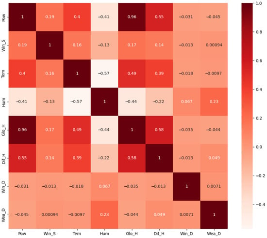
Figure 5.
Correlation analysis between features.
Based on Figure 5, the most correlated features to active power are horizontal and diffuse irradiance, with correlation coefficients of 0.96 and 0.55, respectively. The features used in the experiments presented below were selected based on this correlation analysis.
The ML model proposed was trained with the DKA Solar Center dataset []. Experiment 1 used only the active power feature as input and output. Experiment 2 used active power, wind speed, temperature, humidity, horizontal and diffuse irradiance, wind direction, and weather daily rainfall as input, and active power as output. Experiment 3 used active power, temperature, humidity, horizontal and diffuse irradiance, and wind direction as input, and active power as output.
Experiment 3 used temperature, humidity, global horizontal radiation, diffuse horizontal radiation, and wind direction, based on the features presented in []. The results obtained with the proposed LSMT model are better than the three models (support vector machine, RCC-LSTM, and ESNCNN) tested in [,,]. Another difference is that the LSTM model was trained and tested with three years of data; on the other hand, the SVM model in [] was trained and tested with one year of data.
The optimization metric MSE along each epoch was analyzed in the training model for Experiment 3, and the results are presented in Figure 6. The MSE computed by subsequent epochs shows lesser values after the first epoch. Therefore, the MSE in epoch 10 is smaller than MSE in epoch 1. To show the behavior of the optimization metric MSE in detail, Figure 7 presents a zoomed-in look at MSE vs. each epoch for the training model in Experiment 3.
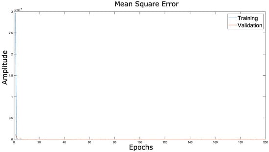
Figure 6.
Optimization function vs. epochs in Experiment 3.
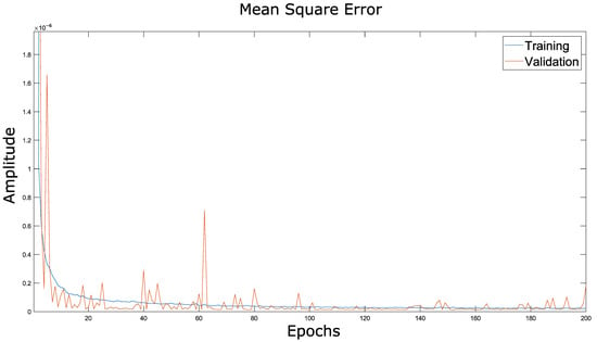
Figure 7.
Optimization function vs. epochs, zoomed in.
A comparison of the original signal , the signal after outlier removal , and the predicted signal is presented in Figure 8. Because the signals and are future values, the signal must be moved one time step into the future.

Figure 8.
Signal comparison using the model trained in Experiment 3.
An additional test was executed using the Ambient Weather Network dataset []. The objective was to assess the proposed ML model’s performance using a dataset with more outliers than DKA and build a baseline model as the first step towards future work focusing on outlier prediction in Puerto Rico. The “UPRM CID Sustainable Energy Center, Mayagüez” device was selected in Puerto Rico, and the records from 20 February 2022 to 6 September 2022 were downloaded. The dataset has 56,340 measures and 18 features. However, Experiment 4 used only solar radiation as input and output. Experiment 4 had an MSE of KW, an RMSE of KW, and an MAE of KW.
The results of Experiment 4 are less accurate than those of the other tests because the Ambient Weather Network dataset has more outliers than the DKA Solar Center dataset. For example, in Figure 9 and Figure 10, both datasets are compared over one day.
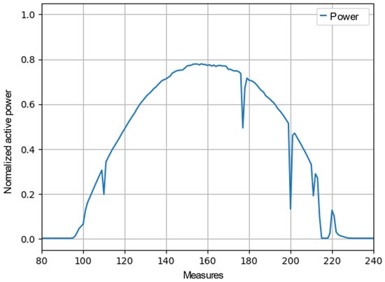
Figure 9.
Outlier references DKA Solar Center Dataset. Normalized active power is on the vertical axis, and the number of measures is on the horizontal axis.
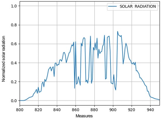
Figure 10.
Outlier references Ambient Weather Network—CID. Normalized solar irradiance is on the vertical axis, and the number of measures is on the horizontal axis.
Experiment 5 work was trained with the DKA Solar Center dataset [], similar to Test 1, but without the outlier detection and removal steps from the proposed workflow, so the input data to train the ML model includes outliers. Experiment 5 had an MSE of KW, RMSE of KW, and MAE of KW.
Experiment 6 used the same subset selected in []: data from the DKA Solar Center dataset [] from January 2018 to December 2019. The subset has 199,097 measures. All of the steps on the model were used, and the results have an MSE of KW, RMSE of KW, and MAE of KW.
Experiment 7 included the DKA Solar Center dataset [] using all of the available data but only the two features most correlated to active power, which were horizontal and diffuse irradiance, with correlation coefficients of 0.96 and 0.55, respectively. All of the steps in the model were used, and the results have an MSE of KW, an RMSE of KW, and an MAE of KW.
The results of all seven experiments and the previous results reported by researchers who worked with the DKA Solar Center dataset [] are presented in Table 4, highlighting the best result in bold.

Table 4.
LSTM model proposed accuracy with the DKA solar center dataset.
5. Discussion
A discussion of the results obtained from the application of the models MISO and SISO LSTM is presented below:
- The MSE metric in Experiment 1, Experiment 2, and Experiment 3 have orders that range from KW to KW. These MSE values are smaller than those presented in [,,], where the MSE value had an order of KW.
- Experiment 1 presented good results using only one input, which reduced the model’s complexity and training time. Typically, the predicted values are only differ slightly from the real values; this error is smaller than 4 Watts in most cases.
- The trained models show good performance regarding signals with low outliers. This model can predict the common behavior of irradiance or power signals in PV systems. However, the proposed model does not produce good predictions regarding measures with sudden fluctuations, because the datasets do not have information on cloud movements to let the ML model anticipate a sudden fluctuation or outlier. Future work will include cloud movement information to train the prediction model to account for these abrupt variations.
- Experiment 3 showed the best results because it used more information than other experiments, but the model used here was more complex than in other experiments.
- Experiment 6 used one year of data, less than other experiments. The objective was to replicate the same conditions as reference []. The results of the proposed model are better than those presented in [,,].
- The results in Table 4 show that adding more features to the ML model does not guarantee better results. For example, Experiment 3, with five features, produced better results with its fewer features than Experiment 2, which has eight features.
- Another example of the previous discussion can be found in Experiment 6 and Experiment 7. Both of these Experiments use the same subset of the dataset, but Experiment 7 has fewer features (only two) than Experiment 6 (five features). However, Experiment 7 achieved better results than Experiment 6. One explanation for this is that more features can introduce noise instead of relevant information; because of this, feature analysis, such as correlation analysis, is an essential part of building ML models.
- The LSTM method outperforms the traditional ML methods used in forecasting problems because LSTM can save and remove information. This was confirmed with Experiment 3, which applied the LSTM method and obtained better results than [], where SVM was utilized.
- In accordance with what was expected, the outlier removal step improved the model’s performance. Comparing Experiment 1, where outliers were removed, to Experiment 5, in which outliers were kept, the results obtained in Experiment 1 were more accurate.
The model developed in this paper will be used to forecast solar irradiance in Puerto Rico, which has a goal of achieving 100% renewable energy by 2050 and where the main renewable energy source is the sun []. Such an aggressive goal requires not only the massive deployment of PV systems but also new ways to plan and operate the local power system. A key aspect to securing the stability of the local grid is to have as clear a prediction as possible of the amount of power that will be available in the near future from the thousands of PV systems spread around the archipelago. The problem becomes more complicated due to Puerto Rico’s location in the Caribbean, where long-term weather predictions have historically been unreliable due to the high variability of winds, the central mountainous region of the main island, the relatively small size of the jurisdiction, and the complicated dynamics of the heat patterns throughout the day from both sea and land.
6. Conclusions
- The preprocessing step and specific feature selection used data correlation analysis. Horizontal irradiance and active power were the most correlated variables, with a correlation coefficient of 0.96. Therefore, horizontal irradiance and active power are the most important features for active power prediction.
- The evaluation of the proposed ML model was conducted via five experiments. The best results were obtained in Experiment 3 with an MSE of KW, an RMSE of KW, and an MAE of KW. These results are better than those presented in [,,].
- Applying HMM for outlier detection and elimination enables the classification of measures without the need for a predefined threshold setup. Outlier detection and elimination improved the results compared to the original signal. This is evident when comparing Experiment 1 to Experiment 5, where Experiment 1 used a signal without outliers as input, whereas Experiment 5 used the original signal as input. The results of Experiment 1 were better.
- The Puerto Rico dataset [] has more outliers than the Australian dataset []. Because of this, the proposed ML model trained with the Australian dataset produced better results than the Puerto Rico dataset. Although this model does not consider outliers, we understand that cloud dynamics can cause dips identified as outliers. Future work will improve the ML model prediction by including outliers.
- The proposed ML method is an excellent tool for reducing the photovoltaic generation planning error implicit in medium- or long-term prediction by updating the generation planning at regular intervals. This enables an energy management system (EMS) to execute necessary actions such as battery charging or utilizing grid energy to maintain high-quality service. However, the proposed ML model does not capture outliers because it requires additional information about cloud movements, which is currently unavailable in the datasets used for this study.
- The outlier detection and elimination strategy using HMM can be used in preprocessing steps for weather datasets and other datasets with time series variables. In addition, the LSTM model can be used in short-term generation planning to complement the information used in EMS and enable proactive response to specific situations, for example, activating batteries when the irradiance decreases below the defined limit.
Author Contributions
Conceptualization, C.J.D., V.M. and E.O.-C.; methodology, C.J.D. and V.M.; software, C.J.D. and E.A.-M.; validation, V.M., E.O.-C. and F.A.; formal analysis, C.J.D. and E.A.-M.; investigation, C.J.D. and E.A.-M.; resources, F.A.; data curation, C.J.D.; writing—review and editing, C.J.D., E.A.-M., V.M., E.O.-C. and F.A.; visualization, C.J.D.; supervision, E.O.-C. and V.M. All authors have read and agreed to the published version of the manuscript.
Funding
This paper is supported by the U.S. Department of Energy under EPSCoR, grant number DE-SC0020281.
Data Availability Statement
The authors confirm that the data used in this work are open access and referenced in this article. The data for DKA-Solar can be accessed via the web page https://dkasolarcentre.com.au (accessed on 11 September 2022), and Ambient Weather can be accessed via https://ambientweather.net/.
Conflicts of Interest
The authors declare no conflicts of interest.
Abbreviations
In order to help understand this paper, the following list of abbreviations summarizes the abbreviations used in the document.
| Abbreviation | Meaning |
| PV | Photovoltaic |
| ML | Machine learning |
| LSTM | Long short-term memory |
| RCC-LSTM | Radiation classification LSTM |
| MSE | Mean square error |
| RMSE | Root mean square error |
| MAE | Mean absolute error |
| HMM | Hidden Markov model |
| TWh | Terawatts by hour |
| ARIMA | Autoregressive integrated moving average |
| MLP | Multilayer perceptron |
| SVM | Support cector machine |
| KNN | K-nearest neighbor |
| AR | Autoregressive |
| ARX | Autoregressive exogenous input |
| CNN | Convolutional neural network |
| ConvLSTM | Convolutional LSTM |
| ARMA | Autoregressive moving average |
| FC-LSTM | Fully connected LSTM |
| MAPE | Mean absolute percentage error |
| ESN | Echo state network |
| R2 | R squared |
| RNN | Recurrent neural network |
| SISO | Single input to obtain a single output |
| MISO | Multiple inputs to obtain a single output |
| DTR | Decision tree |
| NaN | Not a number |
| Pow | Active power |
| Win_S | Wind speed |
| Tem | Temperature |
| Hum | Humidity |
| Glo_H | Global horizontal irradiance |
| Dif_H | Diffuse horizontal irradiance |
| Wind_D | Wind direction |
| Wea_D | Weather daily rainfall |
| UPRM | University of Puerto Rico—Mayaguez |
| CID | Investigation and development center |
| EMS | Energy management system |
References
- Dhar, A.; Naeth, M.A.; Jennings, P.D.; El-Din, M.G. Perspectives on environmental impacts and a land reclamation strategy for solar and wind energy systems. Sci. Total Environ. 2020, 718, 134602. [Google Scholar] [CrossRef] [PubMed]
- Bett, A.; Burger, B.; Friedrich, L.; Kost, C.; Nold, S.; Peper, D.; Philipps, S.; Preu, R.; Rentsch, J.; Stryi-Hipp, G.; et al. Photovoltaics Report. February 2022. Available online: https://www.ise.fraunhofer.de/content/dam/ise/de/documents/publications/studies/Photovoltaics-Report.pdf (accessed on 30 March 2022).
- Hernández-Callejo, L.; Gallardo-Saavedra, S.; Alonso-Gómez, V. A review of photovoltaic systems: Design, operation and maintenance. Sol. Energy 2019, 188, 426–440. [Google Scholar] [CrossRef]
- Fouad, M.M.; Shihata, L.A.; Morgan, E.S.I. An integrated review of factors influencing the performance of photovoltaic panels. Renew. Sustain. Energy Rev. 2017, 80, 1499–1511. [Google Scholar] [CrossRef]
- Gupta, A.; Gupta, K.; Saroha, S. Solar irradiation forecasting technologies: A review. Strateg. Plan. Energy Environ. 2020, 39, 319–354. [Google Scholar] [CrossRef]
- Diagne, M.; David, M.; Lauret, P.; Boland, J.; Schmutz, N. Review of solar irradiance forecasting methods and a proposition for small-scale insular grids. Renew. Sustain. Energy Rev. 2013, 27, 65–76. [Google Scholar] [CrossRef]
- Pan, M.; Li, C.; Gao, R.; Huang, Y.; You, H.; Gu, T.; Qin, F. Photovoltaic power forecasting based on a support vector machine with improved ant colony optimization. J. Clean. Prod. 2020, 277, 123948. [Google Scholar] [CrossRef]
- Patarroyo-Montenegro, J.F.; Vasquez-Plaza, J.D.; Rodriguez-Martinez, O.F.; Garcia, Y.V.; Andrade, F. Comparative and cost analysis of a novel predictive power ramp rate control method: A case study in a pv power plant in puerto rico. Appl. Sci. 2021, 11, 5766. [Google Scholar] [CrossRef]
- Mas’ud, A.A. Comparison of three machine learning models for the prediction of hourly PV output power in Saudi Arabia. Ain Shams Eng. J. 2022, 13, 101648. [Google Scholar] [CrossRef]
- Bacher, P.; Madsen, H.; Nielsen, H.A. Online short-term solar power forecasting. Sol. Energy 2009, 83, 1772–1783. [Google Scholar] [CrossRef]
- Chai, S.; Xu, Z.; Jia, Y.; Wong, W.K. A Robust Spatiotemporal Forecasting Framework for Photovoltaic Generation. IEEE Trans. Smart Grid 2020, 11, 5370–5382. [Google Scholar] [CrossRef]
- Gomez, F.; Sa, N.; Schmidhuber, U.; Wierstra, D. Evolino: Hybrid Neuroevolution/Optimal Linear Search for Sequence Prediction Evolino: Hybrid Neuroevolution/Optimal Linear Search for Sequence Learning. 2005. Available online: https://www.researchgate.net/publication/248554235 (accessed on 13 March 2023).
- Chen, B.; Lin, P.; Lai, Y.; Cheng, S.; Chen, Z.; Wu, L. Very-short-term power prediction for PV power plants using a simple and effective RCC-LSTM model based on short term multivariate historical datasets. Electronics 2020, 9, 289. [Google Scholar] [CrossRef]
- DKA Solar Center. Available online: https://www.dkasolarcentre.com.au (accessed on 11 September 2022).
- Yadav, H.; Thakkar, A. NOA-LSTM: An efficient LSTM cell architecture for time series forecasting. Expert Syst. Appl. 2024, 238, 122333. [Google Scholar] [CrossRef]
- An, W.; Wang, L.; Zhang, D. Comprehensive commodity price forecasting framework using text mining methods. J. Forecast. 2023, 42, 1865–1888. [Google Scholar] [CrossRef]
- Khan, Z.A.; Hussain, T.; Haq, I.U.; Ullah, F.U.M.; Baik, S.W. Towards efficient and effective renewable energy prediction via deep learning. Energy Rep. 2022, 8, 10230–10243. [Google Scholar] [CrossRef]
- Bayrak, F.; Ertürk, G.; Oztop, H.F. Effects of partial shading on energy and exergy efficiencies for photovoltaic panels. J. Clean. Prod. 2017, 164, 58–69. [Google Scholar] [CrossRef]
- Singh, R.; Chen, Y. Learning Gaussian Hidden Markov Models from Aggregate Data. IEEE Control Syst. Lett. 2023, 7, 478–483. [Google Scholar] [CrossRef]
- Lee, J.; Cho, W.; Choi, J. Fault detection for IoT hydrogen refueling station system using a combined hidden Markov model mixed with Gaussian. In Proceedings of the International Conference on Electrical, Computer, Communications and Mechatronics Engineering, ICECCME 2021, Mauritius, 7–8 October 2021; Institute of Electrical and Electronics Engineers Inc.: Piscataway, NJ, USA, 2021. [Google Scholar] [CrossRef]
- Yao, T.; Wang, J.; Wu, H.; Zhang, P.; Li, S.; Xu, K.; Liu, X.; Chi, X. Intra-Hour Photovoltaic Generation Forecasting Based on Multi-Source Data and Deep Learning Methods. IEEE Trans. Sustain. Energy 2022, 13, 607–618. [Google Scholar] [CrossRef]
- Yu, Y.; Si, X.; Hu, C.; Zhang, J. A review of recurrent neural networks: Lstm cells and network architectures. Neural Comput. 2019, 31, 1235–1270. [Google Scholar] [CrossRef] [PubMed]
- Abadi, M.; Agarwal, A.; Barham, P.; Brevdo, E.; Chen, Z.; Citro, C.; Corrado, G.S.; Davis, A.; Dean, J.; Devin, M.; et al. TensorFlow: Large-Scale Machine Learning on Heterogeneous Systems. 2015. Available online: https://www.tensorflow.org/ (accessed on 25 January 2023).
- Ambient, L. Ambient Weather Network. Available online: https://ambientweather.net/ (accessed on 9 February 2023).
- Manu, J. Modern Time Series Forecasting with Python Master Industry-Ready Time Series Forecasting Using Modern Machine Learning and Deep Learning; Packt Publishing Ltd.: Birmingham, UK, 2022. [Google Scholar]
- Rivera, A.A.I.; Colucci-Ríos, J.A.; O’Neill-Carrillo, E. Achievable Renewable Energy Targets for Puerto Rico’s Renewable Energy Portfolio Standard. 2009. Available online: https://bibliotecalegalambiental.files.wordpress.com/2013/12/achievable-renewable-energy-targets-fo-p-r.pdf (accessed on 28 January 2023).
Disclaimer/Publisher’s Note: The statements, opinions and data contained in all publications are solely those of the individual author(s) and contributor(s) and not of MDPI and/or the editor(s). MDPI and/or the editor(s) disclaim responsibility for any injury to people or property resulting from any ideas, methods, instructions or products referred to in the content. |
© 2024 by the authors. Licensee MDPI, Basel, Switzerland. This article is an open access article distributed under the terms and conditions of the Creative Commons Attribution (CC BY) license (https://creativecommons.org/licenses/by/4.0/).