Evaluating Reinforcement Learning Algorithms in Residential Energy Saving and Comfort Management

Abstract

The challenge of maintaining optimal comfort in residents while minimizing energy consumption has long been a focal point for researchers and practitioners. As technology advances, reinforcement learning (RL)—a branch of machine learning where algorithms learn by interacting with the environment—has emerged as a prominent solution to this challenge. However, the modern literature exhibits a plethora of RL methodologies, rendering the selection of the most suitable one a significant challenge. This work focuses on evaluating various RL methodologies for saving energy while maintaining adequate comfort levels in a residential setting. Five prominent RL algorithms—Proximal Policy Optimization (PPO), Deep Deterministic Policy Gradient (DDPG), Deep Q-Network (DQN), Advantage Actor-Critic (A2C), and Soft Actor-Critic (SAC)—are being thoroughly compared towards a baseline conventional control approach, exhibiting their potential to improve energy use while ensuring a comfortable living environment. The integrated comparison between the different RL methodologies emphasizes the subtle strengths and weaknesses of each algorithm, indicating that the best selection relies heavily on particular energy and comfort objectives.

1. Introduction

1.1. Motivation

Contrary to the outdated standpoint considering residents as static constructions, the modern perspective identifies them as multifunctional cyber-physical entities able to provide efficient thermal comfort and promote occupants’ quality of life [1,2,3,4,5]. However, to provide adequate comfort to residents—using the potential integrated heating, ventilation, and air conditioning (HVAC) equipment—a specific amount of energy needs to be consumed. Such an amount portrays a significant portion of the overall energy consumption, rendering residential buildings as energy-intensive consumers and a significant contributor to the surge in greenhouse gas (GHG) emissions [6,7,8]. To this end, to maintain residential comfort in a viable way, the need to harmonize energy conservation while maintaining comfort levels has become an essential objective [9,10,11,12].

For many years, residents relied on manual approaches to control HVAC by adjusting thermostats, opening windows, or turning on fans based on their immediate comfort needs. While these actions provided quick adjustments to the indoor environment, the lack of real-time adaptability often resulted in energy wastage during unoccupied or temperate periods [12,13]. Recognizing this gap, scheduling devices emerged, facilitating pre-configured temperature preferences and timed functions, granting a level of autonomous management while ensuring a stable comfortable environment. However, their static configurations often resulted in energy wastage during, e.g., vacant periods or unforeseen climatic changes, highlighting the necessity of a more sophisticated control mechanism [14].

Following the initial steps in automation, Rule-Based Control (RBC) emerged as the dominant strategy to strike a balance between energy saving and comfort. The utilized rules derived from hands-on observations and expert recommendations, setting actions for specific conditions, like reducing temperatures during off-hours or adjusting ventilation according to occupancy [15]. RBC, however, illustrated numerous limitations, struggling to adapt in real-time to varying factors such as changing weather, fluctuating occupancy, or equipment variations [16]. Additionally, RBC was primarily centered on upholding comfort standards, neglecting energy conservation or financial efficiency. The absence of a holistic understanding of the interplay between various HVAC elements also resulted in less ideal outcomes [16,17,18].

The complexity and unpredictability of managing HVAC led to the rise of algorithm-based control methods, such as RL [19,20,21,22,23]. At its core, RL algorithms learn from interactions with the environment, allowing decisions based on real-time data. Instead of relying on predefined rules such as RBC, RL methodologies continuously refine their strategy, ensuring optimal energy use without compromising comfort. Since residential environments are dynamic—with changing occupancies and external conditions—RL frameworks were adequate to anticipate and respond to different scenarios, whether it is a sudden weather change or varying resident preferences [23,24]. This continuous learning and adaptability mean that RL is sufficient to achieve long-term energy efficiency while always prioritizing the comfort of inhabitants [25,26,27].

However, choosing the optimal RL approach for enhancing energy efficiency in HVAC systems presents a significant challenge [28,29]. Given the dynamic nature of HVAC environments, influenced by fluctuating weather conditions, varying building occupancy, and equipment performance, no single RL algorithm stands out as a universal solution [29]. The plethora of RL algorithms, each tailored to specific scenarios and action spaces, further complicated the selection. The lack of a one-size-fits-all RL solution for HVAC systems suggests that evaluating numerous RL approaches is pivotal in identifying the best-suited strategy for specific applications, such as HVAC systems. Different RL algorithms operate uniquely when controlling residential HVAC due to their varied underlying principles, learning mechanisms, and optimization strategies [23]. Each algorithm is designed with certain assumptions and priorities, which means they respond differently to the dynamic nature of HVAC environments, influenced by fluctuating weather conditions, varying building occupancy, and equipment performance. Some might excel in rapidly changing conditions, while others might be more stable and consistent over longer periods [29]. By comparing different algorithms under consistent conditions, researchers may gain clarity on their respective performances, ensuring evaluations are both fair and insightful [30]. This process highlights the strengths and weaknesses of each algorithm, aiding in making informed decisions. Furthermore, it is not just about finding the best algorithm but understanding how each can be optimized or tailored for specific scenarios.

Motivated by the plethora of RL approaches, current work integrates a comparison between different RL control algorithms towards a conventional RBC approach for exhibiting their adequacy to support an efficient optimal control scheme for balancing energy saving and comfort. To this end, PPO, DDPG, DQN, A2C, and SAC methodologies are thoroughly assessed in a simulative environment for their ability to control the operation of HVAC and thus reduce energy consumption while ensuring indoor comfort. By testing their energy-saving capabilities in a standard residential apartment setting, the research reveals which algorithm stands out as the most suitable.

These algorithms have demonstrated superior performance in similar tasks in previous research, indicating their potential effectiveness for the specific application of HVAC control. Their ability to handle the complexities of an environment like a residential apartment requires balancing between energy saving and comfort. Defining which RL approach balances exploration and exploitation more efficiently is beneficial in finding the optimal control strategies for HVAC and portrays a key factor for the current study. Each of these algorithms has unique strengths and characteristics which render them suitable for the problem of HVAC control for energy saving and comfort. For instance, PPO is known for its stability and reliability in different environments, making it a good choice for applications where safety and consistency are important. DDPG and SAC, being off-policy algorithms, are effective in environments with continuous action spaces, like HVAC control. Another key factor for the selection of the specific set of algorithms was influenced by their practicality in terms of implementation and the availability of support. Algorithms like PPO, DDPG, DQN, A2C, and SAC are often well-documented and supported by popular machine learning frameworks. This makes them more accessible for integration into existing systems, particularly in HVAC applications, fostering potential future real-life deployment.

It should be mentioned, that the concerned RL algorithms are meticulously evaluated against established criteria and user preferences, offering valuable insights into their performance trends. This approach adopts a user-centric perspective, aligning algorithmic control with individual comfort needs and energy efficiency goals, thereby providing customized solutions for various thermal comfort categories. Additionally, by emphasizing the distinct features of each algorithm, the study underscores the significance of choosing the appropriate algorithm based on the specific requirements of the application.

1.2. Related Literature Work

The literature exhibits numerous RL applications in residential buildings for the efficient control of different HVAC equipment. RL approaches such as PPO, DDPG, DQN, A2C, and SAC are commonly utilized to balance energy saving and comfort, reducing costs and the environmental impact on residents. More specifically, in [31], a comparison of the DQN methodology towards a thermostat controller was assessed. The findings indicate that the DQN-enabled intelligent controller surpassed the baseline controller. In the simulated setting, this advanced controller enhanced thermal comfort by approximately 15% to 30% while concurrently achieving a reduction in energy expenses ranging from 5% to 12%. The DQN algorithm in residents was also evaluated in [32], where a data-driven approach was aimed at managing split-type inverter HVACs, factoring in uncertainties. Data from similar AC units and homes were merged to balance out data disparities, and Bayesian convolutional neural networks (BCNNs) were employed to estimate both the ACs’ performance and the associated uncertainties. Subsequently, the Q-learning RL mechanism was established to perform informed decisions about setpoints, using insights derived from the BCNN models. According to the outcome, the novel approach achieved slightly lower energy consumption (19.89 kWh) and discomfort (1.44 °C/h) compared to the rule-based controller [32].

In [33], a DDPG framework was tailored to regulate HVAC and energy storage systems without relying on a building’s thermal dynamics model. This approach took into account a desired temperature bracket and various uncertain parameters. Comprehensive simulations grounded in real-world data attest to the potency and resilience of the suggested algorithm in comparison to the baseline ON/OFF control policy. According to the results, the proposed energy management algorithm was able to reduce the mean value of total energy cost by 15.21% compared to the baseline controller while also achieving a lower mean value of total temperature deviation, indicating improved thermal comfort. Similarly, in [34], researchers employed a dual-focused control strategy for HVAC systems that balanced energy costs with user comfort. By addressing such objectives simultaneously, an optimization model was structured toward energy cost predictions, past usage trends, and external temperatures. Utilizing the DDPG method, an optimal control strategy was achieved that was able to harmonize cost and comfort. According to the results, different weighting factor prices balancing energy cost saving and comfort provided different results. For instance, when the weighting factor reached 0.5, 38.5% energy cost saving was achieved. Increasing the weighting factor to 0.55, energy cost savings reached a 50% improvement in comparison to a predefined temperature schedule control approach. Thermal Comfort Improvement Factor ranged from 42.75% to −28.7% across different weighting factor values.

A comparative analysis between DQN and DDPG methodologies was also carried out to control multi-zone residential HVAC systems in [35]. The concerned optimization objective was twofold: cut down energy expenses and ensure occupant comfort. By using the DDPG method, they effectively learned from continuous interactions in a simulated building setting, even without prior model insights. Their findings reveal that this DDPG-guided HVAC management surpassed the leading DQN, slashing energy costs by 15% and decreasing comfort breaches by 79%. Impressively, when pitted against a conventional RBC method, the DDPG approach reduced comfort infractions by a staggering 98%.

The PPO approach was evaluated in [36] to fine-tune the operation of a building’s HVAC system, aiming to enhance energy efficiency, uphold thermal comfort, and meet set demand response targets. Simulated results showcased that leveraging RL for standard HVAC management was sufficient to achieve energy savings of nearly 22% in weekly energy consumption in comparison to a conventional baseline controller. Furthermore, during periods requiring demand response, employing a controller attuned to demand response with RL can lead to power fluctuations of about 50% over a week, in comparison to a conventional RL controller, all the while ensuring the thermal comfort of the inhabitants.

To assess the effectiveness of deep reinforcement learning (DRL)-based control systems, the researchers conducted evaluations of both PPO and A2C controllers. This evaluation focused on summer cooling performance over one month, followed by a test in the subsequent month using the pre-trained models [37]. Findings indicated that A2C generally outperformed the PPO methodology, particularly with medium-sized network estimation models, except in cool and humid climates, where a PPO control proved more effective. According to the outcome, the A2C control methodology delivered 4% and 22% lower energy consumption concerning the RBC methodology in cooling mode, all while ensuring thermal comfort.

The SAC methodology was evaluated in [38], where the combination of an RL with Long Short-Term Memory (LSTM) neural networks was aimed to steer heat pumps and storage systems across four buildings. Their simulation framework incorporates LSTM models, trained on an artificial dataset from EnergyPlus, to gauge indoor temperature dynamics. The engineered controller effectively sustained comfortable indoor conditions across various buildings, achieving a cost reduction of approximately 3% against the baseline RBC approach. Furthermore, this DRL controller facilitated a peak demand reduction by 23% and decreased the Peak-to-Average Ratio (PAR) by 20%. Additionally, the DRL controller successfully harnessed interactions among diverse sources of flexibility, enhancing the flexibility factor by 4%. Moreover, in [39], the SAC approach was also utilized to efficiently control the thermal storage of a four-building cluster with unique energy profiles. The goal was to optimize individual building energy usage while leveling the overall energy load. When compared to a traditionally set RBC, the novel methodology achieved 4% cost savings, reduced peak demand by up to 12%, and led to a 10% drop in daily average peak, showcasing the benefits of SAC in energy management.

1.3. Novelty

Current work stands out for its comprehensive analysis, exploration of energy and comfort trade-offs, performance evaluation against international standards, user-centric algorithm selection, and detailed characterization of each algorithm. These facets collectively contribute to the novelty and value of our research in advancing the field of residential energy management.

Grounded in a comprehensive analysis of several prominent RL algorithms, namely SAC, PPO, A2C, DDPG, and DQN, within the context of residential energy management, current research evaluates each algorithm’s ability to balance energy efficiency and occupant comfort—a critical consideration in modern living spaces. A key aspect of the current effort lies in exploring the intricate trade-offs between energy reduction and thermal comfort. Such attributes have been achieved by implementing specific weighting parameters—a novel approach that allows us to gauge each algorithm’s performance meticulously. Such attributes not only assess the algorithms based on established criteria, but also factor in user preferences in line with international standards. This approach yields valuable insights into the general trends and performance nuances of the five algorithms under scrutiny, especially regarding how alterations in weight factors and user preferences impact their effectiveness. Moreover, additional emphasis has been given to the scalability and adaptability of these algorithms in different residential settings. Contrary to the majority of the literature, current efforts explore how these RL schemes may be effectively scaled up or down, catering to a wide range of residential environments, from small apartments to large houses, thus broadening the applicability and impact of findings.

Another interesting attribute highlighted in this study concerns the fact that some particular algorithmic schemes, like DQN, may not be directly comparable with others due to their intrinsic mechanisms. Conversely, it is observed that the PPO algorithm consistently maintains lower Predicted Percentage of Dissatisfied (PPD) values, illustrating its adaptability in shifting priorities between objectives. Such observations highlight the necessity of understanding the unique characteristics of each RL algorithm, underscoring the importance of selecting the most appropriate one for specific applications. To this end, contrary to the majority of existing literature approaches, current research does not merely provide a comparative analysis of these algorithms but also delves deep into their traits and suitability for varied applications in residential energy management.

Moreover, current effort enables a user-centric selection of algorithms to empower users to customize algorithmic control and align with their specific comfort needs and energy efficiency objectives. Such attributes pave the way for choosing the most suitable algorithm for each category of thermal comfort, thereby offering personalized solutions. The integration of dynamic user feedback into algorithm performance evaluation is a significant advancement. Unlike traditional static assessments, this approach allows for a more realistic and adaptable evaluation, considering how user preferences can evolve. To this end, current work reflects real-world scenarios accurately, where occupant preferences and comfort levels are not constant but change in response to various factors.

The environmental impact of the current research also concerns a critical aspect. By focusing on energy efficiency and sustainable living, the current study directly contributes to the broader goals of reducing carbon footprints and promoting eco-friendly practices in residential settings. This aligns with global environmental objectives and demonstrates the societal relevance of your work. Last but not least, the potential for real-world implementation and commercialization of these algorithms portrays a fruitful prospect. Current research efforts pave the way for developing new products or services that integrate these advanced algorithms into smart home systems, offering tangible benefits to consumers and industry stakeholders.

1.4. Paper Structure

The paper is structured as follows. In Section 1: Introduction, the motivation of the current work is assessed and the related previous work and the novelty of the current work are elaborated. Section 2: Joint Materials and Methods delivers the general mathematical overview of the RL methodology while providing the conceptual background of the algorithms concerned—PPO, DDPG, DQN, A2C, and SAC—regarding the implementation in HVAC. Section 3: Testbed Description elaborates on the aspects of the concerned simulative testbed description, while Section 4: Results and Discussion illustrates a thorough comparative analysis of RL algorithms’ performance in energy saving and comfort measures. Last but not least, Section 5: Conclusions and Future Work concludes the outcomes of the current study and describes the future work generated by the current research effort.

2. Joint Materials and Methods

This section provides the mathematical description as well as the particularities of RL applications in HVAC control applications. Providing the generalized concept of the RL approach as well as the concept of the individual RL algorithms, the current work aims to establish the landscape of the concerned RL concepts, familiarizing the reader with the current state of the art and highlighting the relevance of the study at hand.

The General Reinforcement Learning Conceptual Background

In RL, an agent interacts with an environment over discrete time steps to achieve a certain objective. At each time step, the agent observes the current state of the environment, which provides a snapshot of all pertinent information about the environment at that moment. Based on this state, the agent selects an action according to its policy. The policy is essentially the strategy or behavior that the agent follows, and it can be deterministic (always giving the same action for a given state) or stochastic (providing a distribution over possible actions) [23,40].

Once the action is taken, the environment transitions to a new state and provides feedback to the agent as a reward (Figure 1). This reward offers a numerical value indicating how good or bad the action was in achieving the agent’s objective. Over time, the agent aims to learn a policy that maximizes its expected cumulative reward, often referred to as the return. To aid in this learning, the agent often estimates a value function, which predicts the expected return from a given state when following a particular policy. This value function helps the agent to judge the long-term consequences of its actions, enabling it to favor actions that lead to higher cumulative rewards in the future [23,40].

More specifically:

• State: The state, denoted as s, encapsulates the current environmental and system-specific conditions that are pertinent to the decision-making process of HVAC control. In the context of HVAC control, the state can be formally represented as [23]:

  $$s=[T_{\mathrm{room}},T_{\mathrm{setpoint}},T_{\mathrm{external}},n_{\mathrm{occupants}},t,\dots ]$$

  (1)

  where $T_{\mathrm{room}}$ is the current room temperature; $T_{\mathrm{setpoint}}$ is the desired temperature; $T_{\mathrm{external}}$ denotes the external temperature; $n_{\mathrm{occupants}}$ is the number of occupants; t represents the current time or time of day.
• Action: The action space encompasses the set of all feasible actions that the HVAC system can take at any given state. Let a denote an action taken by the RL agent. In the HVAC context, this is represented as:

  $$a\in \{\mathrm{ON},\mathrm{OFF},\Delta T_{\mathrm{setpoint}},\Delta \mathrm{airflow}\}$$

  (2)

  where ON and OFF denote the operational status of the HVAC; $\Delta T_{\mathrm{setpoint}}$ represents the adjustment to the temperature setpoint; $\Delta \mathrm{airflow}$ signifies changes in the airflow rate.
• Reward: The reward function provides a quantitative measure of the quality of an action taken by the agent in a particular state. For HVAC systems, the reward function aims to strike a balance between energy efficiency and occupant comfort. Formally, the reward $r(s,a)$ can be defined as:

  $$r(s,a)=-\alpha E_{\mathrm{consumed}}+\beta C_{\mathrm{comfort}}-\delta |T_{\mathrm{room}}-T_{\mathrm{setpoint}}|$$

  (3)

  where $\alpha$, $\beta$, and $\delta$ are weighting parameters; $E_{\mathrm{consumed}}$ is the energy consumed by the HVAC system; $C_{\mathrm{comfort}}$ quantifies the comfort level of occupants.
• Policy: The policy, denoted as $\pi$, provides a mapping from states to actions. It represents the strategy that the RL agent employs to act in the environment. Depending on the RL approach, this policy can be deterministic or stochastic. In deep RL contexts, this policy is often parameterized by a neural network, leading to a functional representation:

  $$a={\pi }_{\theta }\left(s\right)$$

  (4)

  where $\theta$ represents the parameters of the neural network.
• Value Function: The value function offers a prediction of the expected cumulative reward from a given state when following a particular policy. For a policy $\pi$, the value function $V^{\pi }\left(s\right)$ is defined as:

  $$V^{\pi }\left(s\right)={\mathbb{E}}_{\pi }\left[\sum _{t=0}^{\infty }{\gamma }^{t}r(s_t,a_t)|s_0=s\right]$$

  (5)
  Here, $\gamma$ is a discount factor that ensures future rewards are discounted to reflect their temporal delay.

In the context of HVAC control, the goal is twofold: achieve energy saving while maintaining occupant comfort. The state typically captures variables that influence HVAC decisions, such as current room temperature, desired temperature setpoint, external temperature, and the number of occupants. This comprehensive state representation ensures that the RL agent has enough information to make informed decisions. The reward function is designed to balance energy efficiency and comfort. For instance, the agent could receive a positive reward for keeping room temperatures within a comfortable range and a negative reward proportional to the energy consumed. This way, the agent is encouraged to maintain comfort while using as little energy as possible [23,41].

The policy in this scenario maps from the rich state information to HVAC control actions, such as turning the system on/off or adjusting temperature setpoints. As the agent interacts with the environment (the residence and its HVAC system), it refines this policy to better achieve the dual objectives. The value function in the HVAC context provides insights into the long-term benefits of current actions. For instance, turning off the HVAC system might save energy now but could lead to discomfort later, resulting in a lower value. By considering such long-term consequences, the agent is adequate to provide decisions that balance immediate energy savings against future comfort levels [41].

3. Testbed Description

In this study, the simulative testbed concerned a four-floor residential building in Tarragona, Spain, with diverse equipment like thermostats and a central geothermal heat pump, which was integrated into the Energym open-source building simulation library. The setup employed the Stable Baselines3 Python library, creating an environment where the RL agent interacts with the building model, and adjusts thermostat setpoints, while other settings are fixed. The agent’s actions influence the building’s thermal zones, with the environment providing feedback in terms of temperature, humidity, and energy consumption data. A multi-objective reward function guides the agent, balancing energy efficiency and thermal comfort, modifiable by adjusting weight parameters. The setup was benchmarked against a classic temperature control system, fostering a sufficient evaluation of the RL algorithms’ effectiveness in optimizing residential energy management while maintaining occupant comfort.

3.1. Energym Framework

Energym [42] is a Python-based open-source library that is based on both EnergyPlus and Modelica, providing different benchmark building models that are interfaced using the Functional Mockup Interface (FMI) standard. This building framework consists of 11 simulation models providing diverse equipment installments (thermostat, heat pump, battery, air handling unit, electric vehicle, photovoltaic), distinct building usages (apartments, houses, offices, seminar center, and mixed-use), and different methods in the control settings (controlling thermostat setpoints and controlling the equipment directly). In this work, the ApartmentsGrid-v0 case is adopted. This is a residential building located in Tarragona, Spain, consisting of four floors, each of them being an apartment, and there are eight thermal zones (two per floor). The thermal system of the building has a central geothermal heat pump (HP) directly connected to hot water tanks (one per apartment) used only for domestic hot water (DHW) consumption, and to a heating loop providing heat to the entire building. Therefore, regarding the equipment that is present in the building, there are four controllable thermostats (one per floor), a non-controllable heat pump, one battery, and one electric vehicle (EV). The simulation inputs (11 in total) involve thermostat setpoints for the four floors ($P1\_T\_Thermostat\_sp,\dots ,P4\_T\_Thermostat\_sp$), heat pump temperature setpoint ($Bd\_T\_HP\_sp$), temperature setpoints for each tank ($P1\_T\_Tank\_sp,\dots ,P4\_T\_Tank\_sp$), battery charging/discharging setpoint rate ($Bd\_Pw\_Bat\_sp$), and EV battery charging setpoint rate ($Bd\_Ch\_EVBat\_sp$). The output part consists of an extensive set (69 in total) of measurements with respect to the behavior of the building for a given input vector. These simulation outputs provide temperature ($Z01\_T\dots Z08\_T$), humidity, and appliance energy measurements in different zones of the building, supply and return temperature for the heat pump, total energy consumption and HVAC energy consumption ($Fa\_E\_HVAC$), outdoor temperature ($Ext\_T$), and other outputs related to the batteries. For more information about the building ApartmentsGrid-v0, including its thermal zones, components, inputs, and outputs, please refer to the Energym documentation https://bsl546.github.io/energym-pages/sources/apg.html (accessed on 28 November 2023).

3.2. Building Simulative Testbed

The overall workflow contains two gym-based environments which work in conjunction with the well-known Python library, Stable Baselines3 [43]. The chosen model from the Energym framework, i.e., the ApartmentsGrid-v0, serves as a building model that responds with 69 output measurements for a given set of 11 input signals each time, whereas the second gym-based environment, named IntermediateEnv, establishes the interaction between the ApartmentsGrid-v0 and the RL agent implementations of Stable Baselines3. Section 3.3 and Section 3.4 describe the encapsulated operation within IntermediateEnv. Thus, the RL agent is encountered with IntermediateEnv with a Markov property interacting constantly. The overall workflow is depicted in Figure 2. More specifically, the Energym simulation model operates at a fine granularity, running for 480 time steps per day, with each step representing a 3 min interval. This detailed time scale allows for a nuanced simulation of the building environment’s dynamic responses. In contrast, the IntermediateEnv, which facilitates the interaction between the RL agent and the Energym simulation, operates on a coarser time scale. It runs for 48 time steps per day, with each step corresponding to a 30 min interval. This difference in time step granularity is critical for the application of RL actions. Actions determined by the RL agent in the IntermediateEnv are applied to the Energym simulation model and held constant (clamped) for a duration of 10 Energym time steps, cumulatively amounting to 30 min. This approach ensures that each action has a sustained impact on the building environment, allowing the system enough time to reach a more stable state in response to the action. Also, it ensures that the system’s response is not merely a transient reaction to the changes but rather a reflection of a more settled state. Such a setup is important in evaluating the effectiveness of the RL algorithms over a realistically significant duration, accurately capturing the implications of each action on energy consumption and thermal comfort in the simulated building.

As mentioned, Energym includes a wide set of input and output measurements on this specific building. The utilized input and output signals are depicted in

Table 1. Action signals of the RL agent.

Parameter Description	Parameter Description	Symbol in Energym	Symbol in This Work
Thermostat setpoints for floors 1 to 4 (°C)	[16, 26]	$P\left\{\mathbf{X}\right\}\_T\_Thermostat\_sp$	$Thermosta{t}_{\left\{\mathbf{X}\right\}}$
Heat pump temperature setpoint (°C)	[35, 55]	$Bd\_T\_HP\_sp$	$Heatpump$
Temperature setpoints for tanks 1 to 4 (°C)	[30, 70]	$P\left\{\mathbf{X}\right\}\_T\_Tank\_sp,$	$Tan{k}_{\left\{\mathbf{X}\right\}}$
Battery charging/discharging setpoint rate	[−1, 1]	$Bd\_Pw\_Bat\_sp$	$Batter{y}_{rate}$
EV battery charging setpoint rate	[0, 1]	$Bd\_Ch\_EVBat\_sp$	$EVBatter{y}_{rate}$

and

Table 2. Subset of output measurements (state signals) from the building model that are inserted in the IntermediateEnv.

Parameter Description	Parameter Description	Symbol in Energym	Symbol in This Work
Zone temperatures for zones 1 to 8 (°C)	$Z0\left\{\mathbf{X}\right\}\_T$	[10, 40]	$Tem{p}_{zone\left\{\mathbf{X}\right\}}$
Outdoor temperature	$Ext\_T$	[−10, 40]	$Tem{p}_{ext}$
HVAC energy consumption (Wh)	$Fa\_E\_HVAC$	[0, 2000]	$E^{cons}$

, respectively. Note that we change the notation of these measurements. To enhance the comprehensibility of the actions and states within our experimental setup, we have opted to use descriptive names that differ from the original Energym nomenclature. This decision was made to ensure clarity and ease of understanding for readers not familiar with the specific terminologies of the Energym platform.

3.3. Actions and State

The ongoing interaction between the agent and the environment involves the agent selecting actions, to which the environment responds by providing rewards and introducing new states for the agent to consider. The action is of the following form:

$$\begin{array}{c}action=\left\{\begin{array}{ccccc}(Thermosta{t}_1& \dots & Thermosta{t}_4),& Heatpump,& \end{array}\right.\dots \hfill \\ \dots ,\left.\begin{array}{ccccc}(Tan{k}_1& \dots & Tan{k}_4),& Batter{y}_{rate},& EV Batter{y}_{rate}\end{array}\right\}\hfill \end{array}$$

(6)

where $(Thermosta{t}_1\dots Thermosta{t}_4)$ represent the thermostat setpoints for each floor, $Heatpump$ is the heat pump temperature setpoint that constantly takes a mean value in its operating bounds, $(Tan{k}_1\dots Tan{k}_4)$ are the tank temperature setpoints for each floor constantly taking a mean value of their operating bounds, $Batter{y}_{rate}$ stands for the battery charging/discharging setpoint rate that is constantly zero, and $EVBatter{y}_{rate}$ is the EV battery charging setpoint rate that is also zero every time. The action variables that are left free to be adjusted/trained by the agent are the four thermostats, while the remaining setpoints for the tanks and the heat pump constantly take a mean operating value. In this work, we leave aside the electrical parts of the battery and EV battery, so these values will constantly be zero throughout the interaction with the building model. Thus, the action space is completely aligned with the input space of the ApartmentsGrid-v0 building model. As mentioned, the building model returns 69 measurements for a given action vector. The observation space is a subset of those building responses. The state variables are defined as follows:

$$state=\{(Tem{p}_{zone1}\dots Tem{p}_{zone8}),Tem{p}_{ext},E^{cons}\}$$

(7)

where $(Tem{p}_{zone1}\dots Tem{p}_{zone8})$ and $Tem{p}_{ext}$ represent the temperature measurements in degrees Celsius for the eight different building zones and outdoor conditions, respectively, and $E^{cons}$ stands for the HVAC energy consumption, which is also measured continuously.

3.4. Reward Function

The objective here is to reduce energy consumption while sustaining thermal comfort for occupants controlling solely the thermostats of the building. Indeed, two contradictory factors together formulate the multi-objective reward function. Thus, the reward function is defined as:

$$reward=\{\alpha \left[E^{cons}\left(t\right)\right]-\beta \left[T{h}^{com}\left(t\right)\right]\}$$

(8)

where $E^{cons}\left(t\right)$ is the HVAC energy consumption that is straightforwardly measured from the building at each time instance, while $T{h}^{com}\left(t\right)$ is directly connected with the thermal comfort index. The emerging trade-off between HVAC energy consumption and thermal comfort is shifted into the tuning process of parameters $\alpha$ and $\beta$ in reducing the first factor as much as possible while sustaining acceptable levels of comfort with minimum penalty. Different weights between the two tuning parameters present different results in favoring either the first or the second reward sub-term. In this work, we keep $\beta =(1$ − $\alpha )$, considering three weight sets $\{0.1,0.5,0.9\}$ towards testing three different operational modes. The intermediate scenario (weight = $0.5$) induces a balance between the two reward factors, while the other two cases maintain slightly extreme cases that focus on either reducing electricity bills with a large thermal comfort penalty or increasing high levels of thermal comfort regardless of energy consumption.

3.5. Baseline Classic Controller Description

To evaluate the effectiveness of the adopted RL controllers, it is essential to compare their performance against a traditional, established control system. For this purpose, we utilize a classic controller, as implemented in the Energym framework, to serve as our baseline. This controller operates on a simple yet effective principle; it maintains a specified indoor temperature within a defined tolerance range. The operational mechanism of this classic controller is straightforward. It requires a set temperature and a tolerance limit. Whenever the indoor temperature deviates from the set value by more than the tolerance (in absolute terms), the controller activates to restore the temperature to the predetermined level. For our comparative analysis, we have set the average indoor temperature to 20.375 °C. This setpoint is coupled with a tolerance of 0.3 °C to allow for minor fluctuations without triggering the control mechanism unnecessarily.

During the operation of the classic controller, we observed an average PPD index of 5.9%. This metric provides insight into the level of thermal comfort experienced by occupants and is crucial for assessing the practicality of the control strategy from a human-centric perspective. In terms of energy efficiency, the classic controller showed an average energy consumption of 430.183 Wh per time step. This consumption rate is a critical benchmark for evaluating the energy performance of our RL controllers under identical conditions. By comparing the performance of the RL controllers with this classic controller, we aim to ascertain not only their relative energy efficiency but also their ability to maintain occupant comfort, thereby determining their viability for practical applications in building energy management.

3.6. Thermal Comfort Metrics

The energy consumption of buildings is significantly influenced by various factors, such as indoor environmental conditions (including temperature, ventilation, and lighting) and the design and operation of the building and its systems. Simultaneously, these indoor conditions have a profound impact on the well-being, performance, and overall satisfaction of occupants within the built environment. It has been established that maintaining high-quality indoor environmental conditions can enhance work and learning performance, reduce absenteeism, and increase overall comfort. In addition, occupants who experience discomfort are more inclined to take actions to enhance their comfort, which might have implications for energy usage. Consequently, there is an increasing demand for well-defined criteria to guide building design and energy assessments [44]. To address these concerns, a series of indices have been developed, rigorously tested, and implemented to evaluate and optimize the indoor thermal environment. The wide set of international standards in this area include (i) ASHRAE 55 [45]—thermal environment conditions for human occupancy; (ii) ISO 7730 [46]—ergonomics of the thermal environment and analytical determination and interpretation of thermal comfort using calculation of the Predicted Mean Vote (PMV) and Predicted Percentage of Dissatisfied (PPD) and local thermal comfort effects; (iii) EN 16798 [47]—specification of criteria for measurements and methods for long-term evaluation of the indoor environment obtained as a result of calculations or measurements.

Thermal comfort assessment is a multifaceted process that takes into account several critical factors and aims to predict how a group of individuals perceives their thermal environment. This involves considering environmental parameters, including relative humidity (RH) and dry-bulb air temperature (tdb), and individual variables such as total clothing insulation (Icl) and metabolic rate (M). The PMV is the established reference for assessing thermal comfort in mechanically conditioned buildings, serving as a tool to anticipate individuals’ perceptions of their thermal environment. For naturally conditioned buildings, the adaptive models of EN and ASHRAE are utilized. The PPD index provides insight into the percentage of people likely to feel too warm or too cool. Figure 3 illustrates the thermal sensation scale and the representation of PPD as a function of PMV [48,49]. The PMV values correlate with the PPD index, highlighting the balance between thermal comfort and dissatisfaction.

The application of these comfort models in practical scenarios is detailed in

Table 3. Different levels of criteria regarding thermal comfort based on EN 16798-2 standard [47].

Category	PPD %	PMV	Description
I	<6	$-0.2<PMV<+0.2$	High level of expectation and also recommended for spaces occupied by very sensitive and fragile persons with special requirements like some disabilities, sick, very young children, and elderly persons, to increase accessibility.
II	<10	$-0.5<PMV<+0.5$	Normal level of expectation.
III	<15	$-0.7<PMV<+0.7$	An acceptable, moderate level of expectation.
IV	<25	$-1.0<PMV<+1.0$	Low level of expectation. This category should only be accepted for a limited part of the year.

. The table categorizes levels of thermal comfort expectation, delineating the acceptable PMV ranges and corresponding PPD percentages, which formulate the assessment metrics for building thermal comfort. These categories range from Category I, which signifies a high level of thermal comfort expectation suitable for sensitive groups (expectation with less than 6% predicted dissatisfaction), to Category IV, indicating a lower expectation that is considered acceptable for only part of the year.

4. Results and Discussion

This section delves deeper into the comparative performance of various RL algorithms in the context of a multi-objective reward function focusing on energy consumption and thermal comfort. In the context of the classic controller, with an average energy consumption of 430.183 Wh per time step and an average PPD of 5.9%, these RL algorithms demonstrate a range of performances. This comparative analysis highlights the strengths and limitations of each RL algorithm in balancing energy efficiency and occupant comfort. Such insights are vital for selecting the most suitable algorithm for specific building environments and occupant needs, ultimately contributing to more intelligent and sustainable building management systems. The performance of these algorithms, as shown in

Table 4. Performance comparison after 5 distinct runs for each algorithm.

Weight Case	RL Algorithm	Average HVAC Energy Consumption (Wh)	Average PPD (%)	Average Power Diff (%)
	SAC	119.0829	25.11	72.32
	PPO	307.7933	6.54	28.45
w = 0.1	A2C	82.4841	34.91	80.83
	DDPG	191.3231	24.40	55.53
	DQN	318.9417	7.78	25.86
	SAC	258.8230	9.63	39.83
	PPO	297.7426	6.8	30.79
w = 0.5	A2C	320.5797	7.04	25.48
	DDPG	214.5196	25.15	50.13
	DQN	507.4004	7.27	−17.95
	SAC	258.6270	8.68	39.88
	PPO	314.7583	6.50	26.83
w = 0.9	A2C	301.9630	6.92	29.81
	DDPG	199.7418	25.08	53.57
	DQN	467.2232	6.30	−8.61

, is evaluated under different weight scenarios (w = 0.1, w = 0.5, and w = 0.9) that prioritize either energy reduction or thermal comfort to varying degrees. The average values for each algorithm presented in Table 4 are derived from five distinct evaluation runs for generalization purposes. For metrics such as Predicted Percentage Dissatisfied (PPD), the average is computed across the building’s eight zones, providing a comprehensive view of the occupant’s comfort throughout the entire building. This methodical approach to averaging ensures that the reported values accurately reflect the overall performance of the algorithms in varying spatial contexts within the simulated environment. Note that the architecture and hyper-parameter configuration of the utilized RL algorithms are presented in Appendix B, i.e.,

Table A1. A2C hyperparameter configuration.

Parameter	Default Value
Learning Rate	$7\times {10}^{-4}$
Number of Steps per Rollout	5
Discount Factor ($\gamma$)	0.99
Neural Network Architecture	2 layers, 64 neurons each
Entropy Coefficient	0.01

,

Table A2. DDPG hyperparameter configuration.

Parameter	Default Value
Learning Rate	$1\times {10}^{-3}$
Batch Size	100
Discount Factor ($\gamma$)	0.99
Neural Network Architecture	2 layers (400, 300 neurons)
Replay Buffer Size	1,000,000
Polyak Coefficient (Tau)	0.005
Exploration Noise (Std Dev)	0.2
Noise Clip	0.5

,

Table A3. DQN hyperparameter configuration.

Parameter	Default Value
Learning Rate	$1\times {10}^{-4}$
Batch Size	32
Discount Factor ($\gamma$)	0.99
Neural Network Architecture	2 layers, 64 neurons each
Replay Buffer Size	1,000,000
Exploration Strategy (Epsilon)	Start: 1.0, End: 0.05
Target Network Update Frequency	1000 steps
Learning Starts	5000 steps

,

Table A4. SAC hyperparameter configuration.

Parameter	Default Value
Learning Rate	$3\times {10}^{-4}$
Batch Size	256
Discount Factor ($\gamma$)	0.99
Neural Network Architecture	2 layers, 256 neurons each
Polyak Coefficient (Tau)	0.005

and

Table A5. PPO hyperparameter configuration.

Parameter	Default Value
Learning Rate	$3\times {10}^{-4}$
Batch Size	64
Discount Factor ($\gamma$)	0.99
Neural Network Architecture	2 layers, 64 neurons each
Number of Epochs	10
Clip Range	0.2
GAE Lambda	0.95
Value Function Coefficient	0.5
Entropy Coefficient	0.01
Number of Steps per Rollout	2048

.

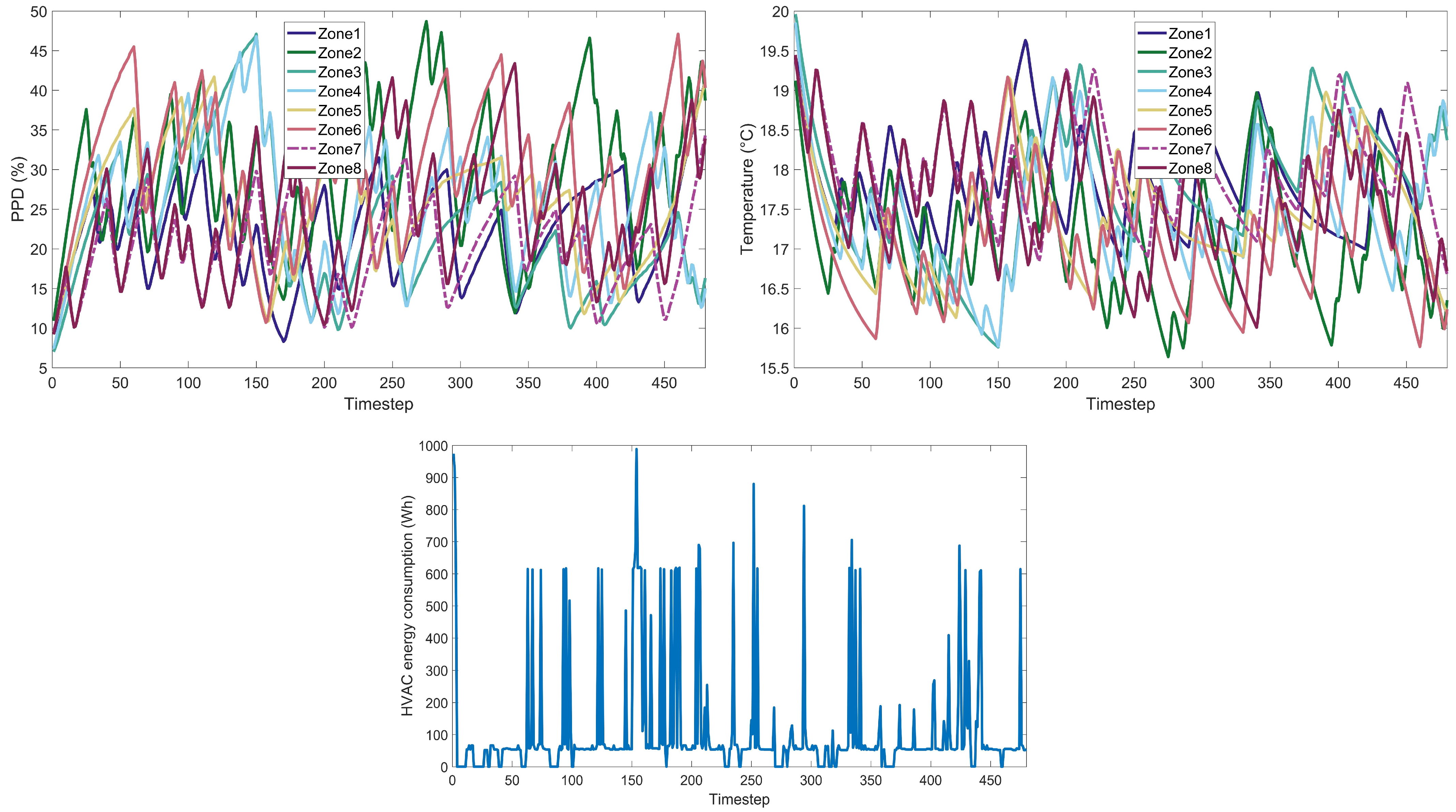
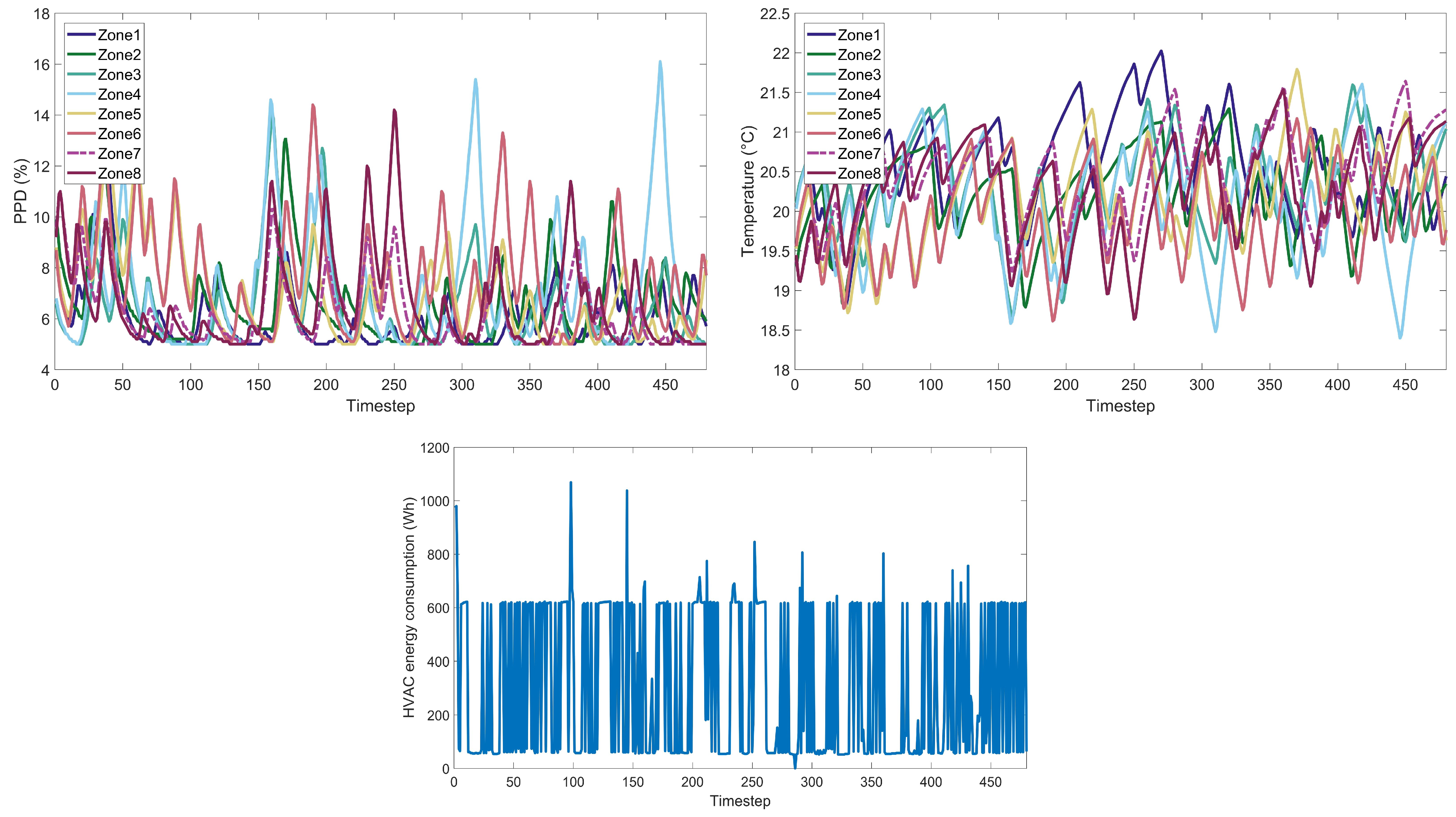
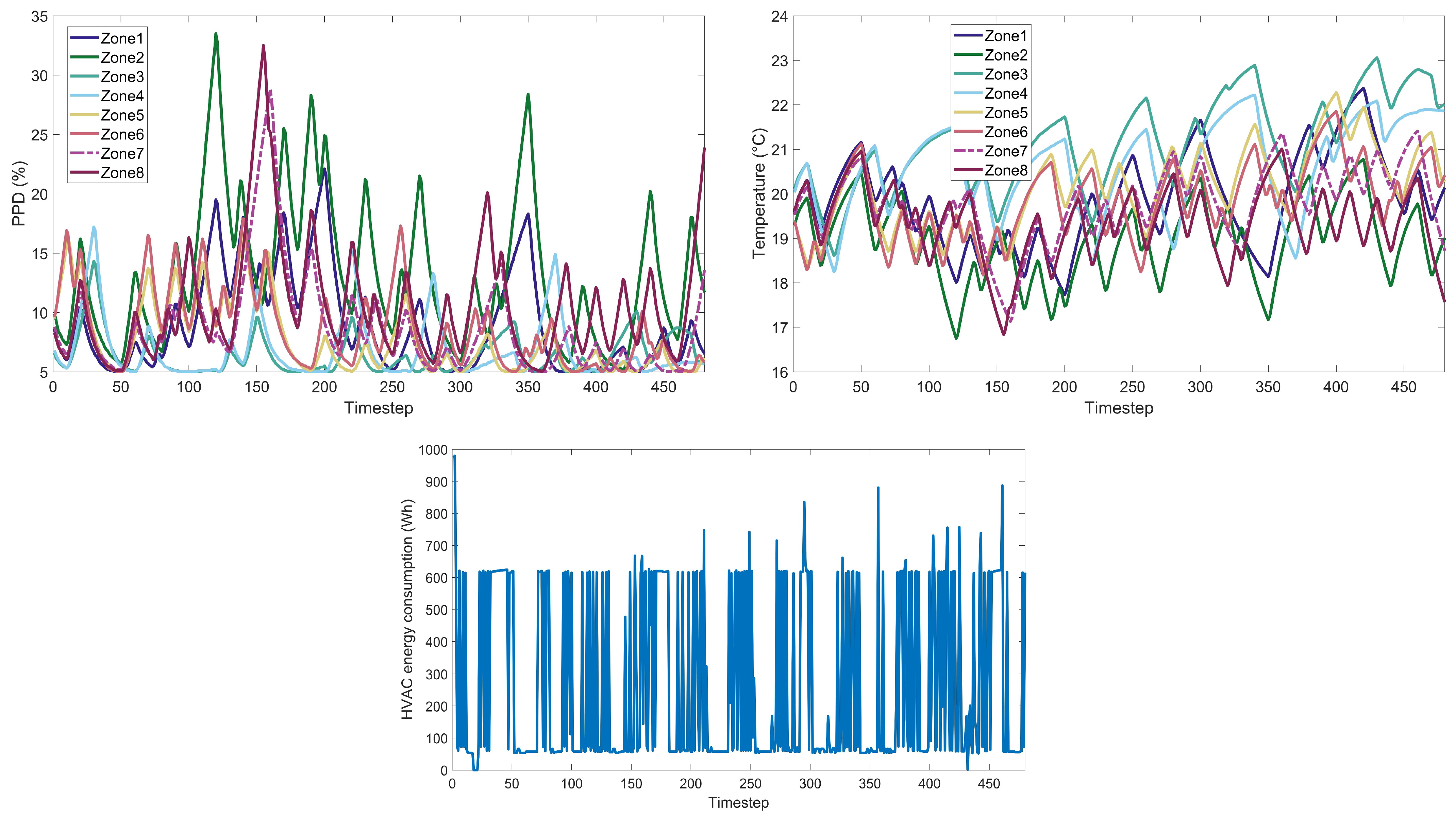
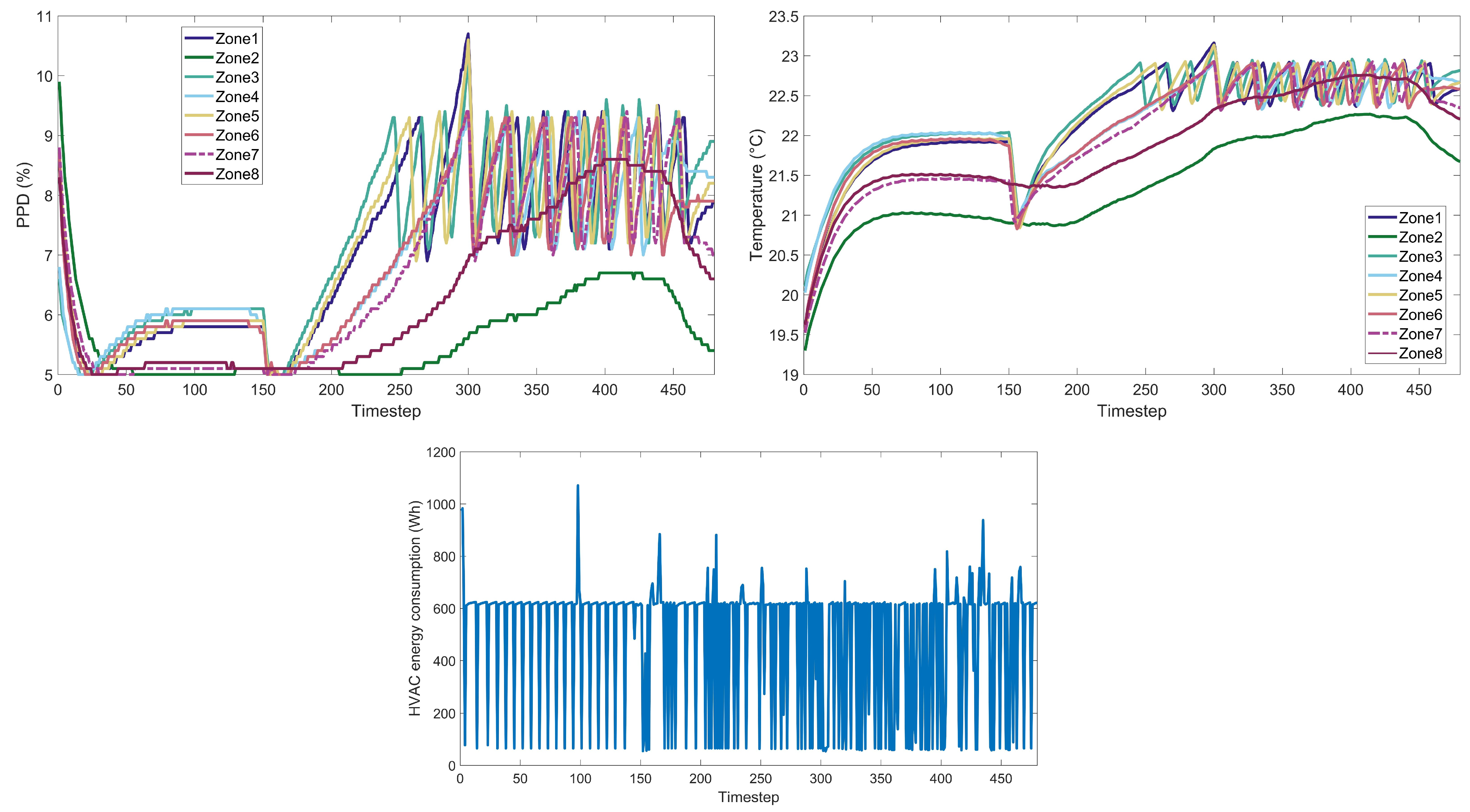
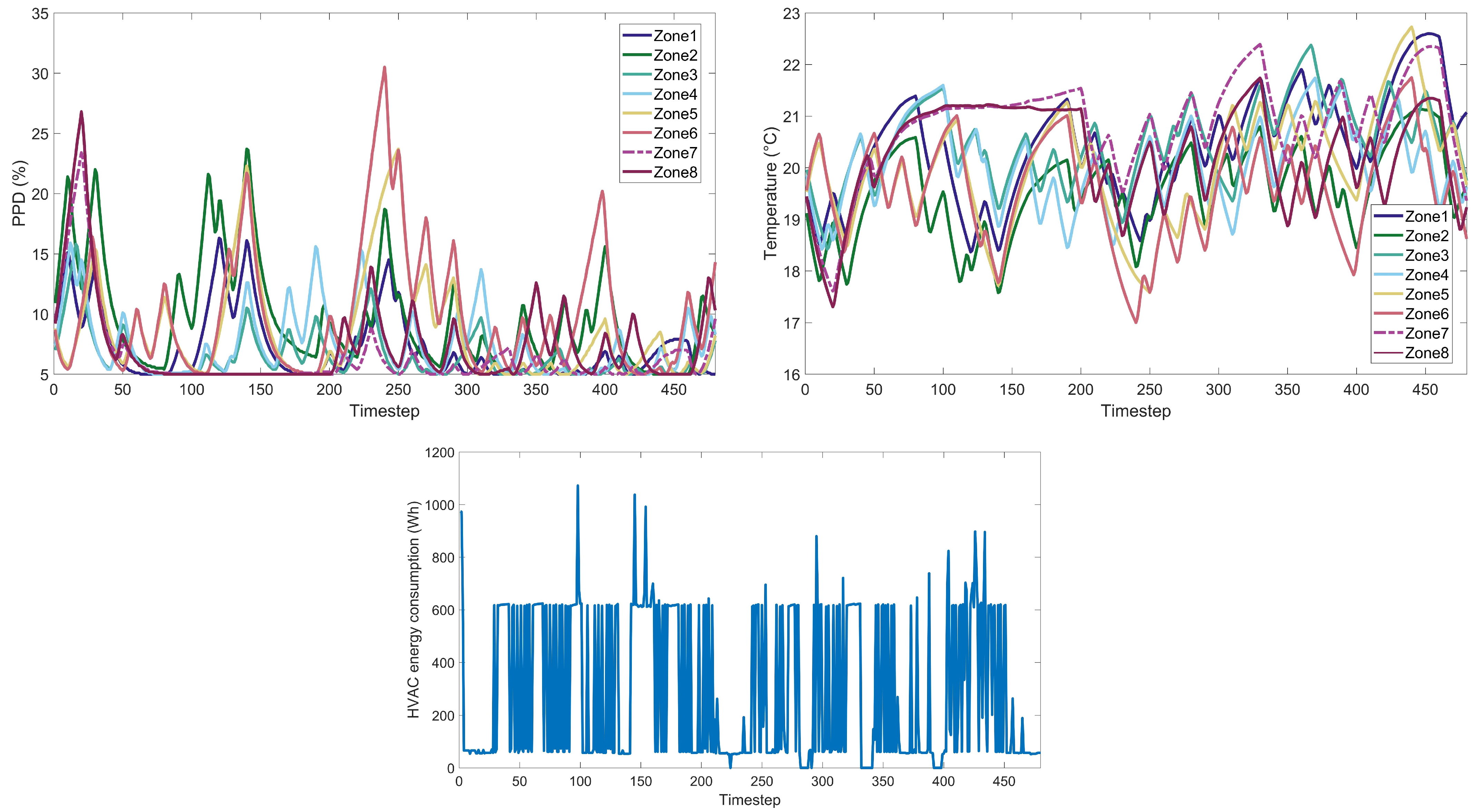
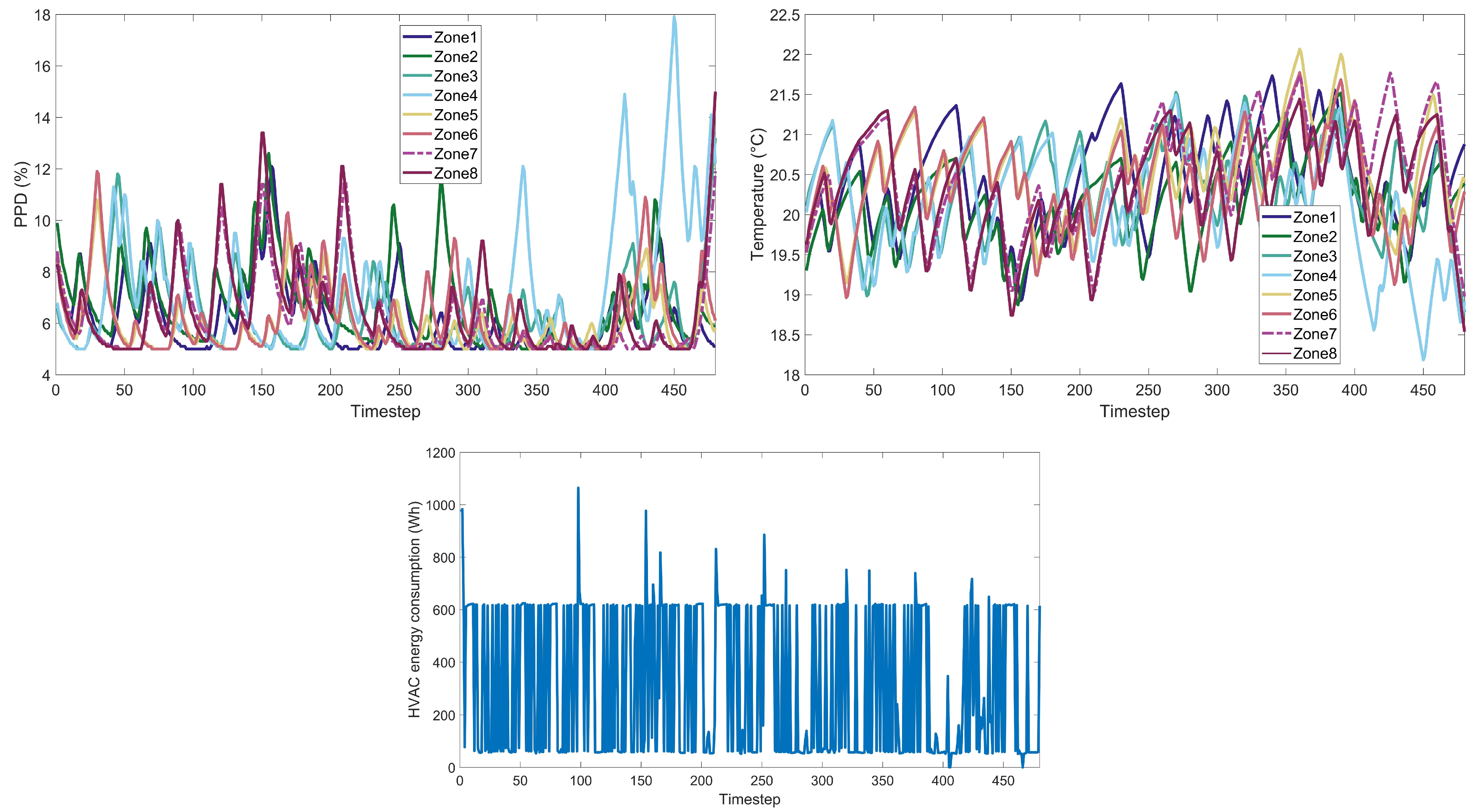
In Appendix C, we provide a comprehensive collection of supplementary results (see Figure A1, Figure A2, Figure A3, Figure A4, Figure A5, Figure A6, Figure A7, Figure A8, Figure A9, Figure A10, Figure A11, Figure A12, Figure A13, Figure A14 and Figure A15) that encapsulate the extensive simulations conducted across various algorithmic cases. For each RL algorithm examined, we present detailed visual data under different weight scenarios, including (a) the Predicted Percentage Dissatisfied (PPD) for each thermal zone within the building, offering insights into the thermal comfort levels achieved; (b) the measured temperature for each building zone, which illustrates the algorithms’ performance in maintaining the desired thermal conditions; (c) the HVAC energy consumption throughout the day, providing a quantitative measure of the algorithms’ energy efficiency. This ensemble of 45 images serves to augment the empirical findings discussed in the main text, allowing for a granular assessment of each RL algorithm’s ability to navigate the trade-offs between thermal comfort and energy consumption. By presenting these data visually, we aim to facilitate a deeper understanding of the nuanced performance characteristics of each algorithm within a residential building energy management context.

4.1. Weight Implications on Performance

The weight factor in the reward function plays a crucial role in balancing between reducing energy consumption and maintaining thermal comfort, specifically:

Weight 0.1: This weight setting places a higher emphasis on energy reduction. Algorithms operating under this weight are expected to minimize energy usage, potentially at the expense of occupant comfort.

Weight 0.5: Represents a balanced approach, giving equal importance to both energy savings and maintaining a satisfactory PPD level.

Weight 0.9: Prioritizes thermal comfort, aiming to achieve a PPD level close to 6%, akin to the performance of the classic controller, and aligning with the standards of Category I, which represents a high level of thermal comfort expectation.

4.2. Analysis of RL Algorithms

Each RL algorithm demonstrates unique characteristics under the aforementioned weight settings:

Soft Actor-Critic (SAC): Under weight 0.1, SAC significantly reduces energy consumption but with a higher PPD, indicating a compromise in comfort. As the weight shifts towards thermal comfort (w = 0.9), SAC shows a balance, maintaining lower energy consumption while keeping the PPD close to the desired 6%. This performance makes SAC particularly suitable for environments that require normal levels of thermal comfort. Its ability to achieve a relatively low PPD while also providing substantial energy savings exemplifies its applicability in scenarios where both comfort and energy efficiency are important, but a perfect balance is not critical (like Category II).

Proximal Policy Optimization: PPO demonstrates moderate energy consumption across all weight settings, with consistently lower PPD values, indicating a steady performance in balancing energy efficiency and comfort. One of PPO’s strengths is its ability to achieve lower PPD values, which is indicative of higher occupant thermal comfort. This is particularly significant in settings where maintaining a comfortable indoor environment is as important as energy efficiency. PPO shows a commendable adaptability to varying weights in the reward function. Whether the focus is on energy efficiency or thermal comfort, PPO adjusts its strategy accordingly, showcasing its flexibility. Perhaps the most notable aspect of PPO is its balanced approach to energy efficiency and occupant comfort. Unlike some algorithms that may excel in one aspect but fall short in the other, PPO provides a harmonious balance, making it a versatile choice for a wide range of applications. Another aspect is related to the reliability it offers. In terms of operational predictability and reliability, PPO presents fewer fluctuations in performance metrics, which is beneficial for long-term planning and consistent building management operations. However, it is crucial to recognize that due to its intrinsic algorithmic design, PPO inherently lacks the granularity to precisely adjust the equilibrium between energy saving and thermal comfort objectives in this formulated problem. PPO is influenced by the reward function’s design, neural network architecture, and entropy term. Adjustments to these factors can help fine-tune the algorithm’s policy, potentially improving adherence to desired comfort levels. This limitation subtly guides its performance to align more closely with scenarios characteristic of Category I, irrespective of the weight variations in the reward function. PPO’s operational framework, therefore, inherently favors occupant comfort optimization, a trait that becomes increasingly apparent under diverse reward function conditions. This inclination towards maintaining lower PPD values, despite shifts in prioritization, highlights PPO’s aptness for environments where thermal comfort is paramount, yet also underscores a potential limitation in settings where a distinct emphasis on energy efficiency, with a more flexible balance, is essential.

Advantage Actor-Critic: At a weight of 0.1, A2C demonstrates the lowest energy usage among all tested algorithms, highlighting its strong inclination towards energy conservation, but with the highest PPD, suggesting a strong bias towards energy saving over comfort. As the weight shifts towards prioritizing thermal comfort (such as at weight 0.9), A2C shows a slight improvement in maintaining comfort levels. However, this improvement is marginal, suggesting that while A2C can adapt to different priorities, its strength lies predominantly in energy saving with a small fraction of penalty in thermal comfort. A2C’s performance profile makes it a decent candidate for energy-critical applications, especially in scenarios where energy budgets are tight, and slight compromises in comfort can be tolerated. One of A2C’s advantages is its predictability in energy-saving outcomes, making it a reliable option for long-term energy management strategies where consistent low energy usage is paramount.

Deep Deterministic Policy Gradient: DDPG’s performance in terms of PPD and energy consumption remains relatively consistent across different weight settings, as indicated by its PPD values ranging from 24.4% to 25.15%. However, it is important to note that these PPD values, hovering around 25%, signify a lower level of occupant thermal comfort, aligning more with Category IV standards (Low Expectation, $PPD<25\%$). While DDPG demonstrates a certain level of stability in its performance, it does so at a relatively lower standard of thermal comfort. This aspect is crucial for applications where higher thermal comfort is a priority.

Deep Q-Network: The performance of the DQN algorithm across different weights suggests a tendency towards higher energy consumption without proportionate gains in thermal comfort with an exception to w = 0.1, where it provides an adequate energy reduction with a small penalty on thermal comfort. Even at a weight of 0.9, where the focus is more on comfort, DQN consumes considerably more energy compared to the classic controller (−8.61%), while achieving only marginally better PPD values (6.3%). This trend is more pronounced at weights 0.5 and 0.9, where DQN’s energy consumption far exceeds the baseline set by the classic controller, indicating inefficiency. This suggests that DQN, despite its potential to achieve lower PPD values, does so at a significant energy cost, making it less suitable for applications where energy efficiency is a priority or where a balance between energy consumption and thermal comfort is desired. The inherent design of DQN, particularly its approach to discretizing the action space, might be a contributing factor to its performance characteristics. Non-continuous discretization can limit the algorithm’s ability to fine-tune its actions for optimal performance, potentially leading to higher energy consumption and only marginal improvements in thermal comfort.

4.3. Overall Comparison and Implications

The analysis reveals a diverse range of responses from each RL algorithm to the prioritization of energy reduction versus thermal comfort. PPO and A2C exhibit a more balanced approach across different weights, suggesting their suitability for scenarios where both energy efficiency and comfort are equally prioritized. SAC and A2C are the most energy-efficient but they heavily compromise comfort in the w = 0.1 scenario. On the other hand, these two algorithms produce the desired performance on the other two weighting scenarios in both objective metrics. DDPG and DQN appear more inclined towards optimizing comfort, especially at higher weights, leading to degraded models.

However, it is essential to identify the best-performing algorithm for each thermal comfort category based on the results to provide clear guidance on which RL algorithms are most suitable for different levels of thermal comfort expectations, from the most strict (Category I) to the least (Category IV). Thus, the best-performing RL algorithms for each thermal comfort category, considering both energy consumption and PPD values, as follows:

Category I (High Expectation, $PPD<6\%$): For this category, where a high level of thermal comfort is expected, the algorithm that maintains PPD closest to $6\%$ with the lowest energy consumption is ideal. In our results, PPO and A2C stand out as the most suitable choices, balancing energy efficiency while maintaining a high level of comfort. More specifically, the lowest achieved PPD values are 6.5% and 6.92% for PPO and A2C, respectively, under weight case w = 0.9, providing energy reduction of 26.83% and 29.81%. Both PPO and A2C demonstrate their capability to operate effectively in scenarios demanding stringent comfort requirements, as defined by Category I. Their performances suggest that they can achieve near-optimal thermal comfort levels while also contributing to energy savings, making them well-suited for applications where occupant comfort is a paramount concern, but energy efficiency cannot be overlooked.

Category II (Normal Expectation, $PPD<10\%$): Here, the acceptable level of discomfort is slightly higher but still lies within the normal level of expectation. Thus, algorithms that can maintain PPD below $10\%$ while optimizing energy consumption are preferred. SAC demonstrates a commendable balance between energy efficiency and thermal comfort. In our results, under the weight case w = 0.9, SAC achieved a PPD of 8.68%, which is within the acceptable range for Category II. Moreover, it managed to reduce energy consumption by nearly 40% (39.88%), indicating its effectiveness in optimizing energy usage while maintaining a reasonable level of occupant comfort. This performance makes SAC particularly suitable for environments that require normal levels of thermal comfort. Its ability to achieve a relatively low PPD while also providing substantial energy savings exemplifies its applicability in scenarios where both comfort and energy efficiency are important, but a perfect balance is not critical.

Category III (Moderate Expectation, $PPD<15\%$): Based on the produced results, no case lies within the PPD range of [10%, 15%), so the selected algorithm would still be SAC. We should select an algorithm that keeps the PPD within this threshold while optimizing energy consumption. Looking at the data, SAC with weight 0.9 could be a better fit for Category III, as it has a PPD of 8.68%, which is within the threshold, and offers a reasonable energy reduction of 39.88%.

Category IV (Low Expectation, $PPD<25\%$): This category allows for a higher level of discomfort in favor of energy savings, but the PPD still needs to be below 25%. DDPG with weight 0.1 might be a suitable option for Category IV, as it has a PPD of 24.4%, which is within the threshold, and an average HVAC power of 191.3231 Wh, indicating high energy efficiency (55.53% consumption reduction with respect to classic controller).

Figure 4 provides a visualized representation of Table 4 to easily compare the trade-offs between energy savings and thermal comfort provided by each algorithm under different preference weightings, giving a clear picture of which algorithms are more suitable for certain comfort categories and energy efficiency objectives. The data points are color-coded and shape-coded for each RL algorithm across three different weight conditions (w = 0.1, w = 0.5, and w = 0.9). The lines with arrows are intended to depict the trajectory from energy reduction towards thermal comfort for each RL algorithm as the weighting factor changes from w = 0.1 to w = 0.9. This way, the arrows represent the direction of increasing weight on the PPD in the reward function, moving from right to left on the graph.

This categorization approach allows for a targeted selection of RL algorithms based on specific thermal comfort requirements and energy efficiency goals. It enables the implementation of more nuanced and effective building management strategies, catering to the varying needs of building occupants and operational efficiency mandates. In the broader context of multi-objective optimization in building management, these insights are critical. They not only inform the selection of appropriate algorithms for specific building environments but also highlight the inherent trade-offs between energy efficiency and occupant comfort. This understanding is pivotal for developing intelligent and sustainable building management systems that align with various occupant needs and environmental sustainability goals.

5. Conclusions and Future Work

The current study presents a comprehensive analysis of five prominent RL algorithms—PPO, DDPG, DQN, A2C, and SAC—in the context of residential energy management, with a focus on balancing energy efficiency and occupant comfort. The research stands out for its in-depth evaluation of these algorithms’ performance in maintaining energy efficiency while ensuring thermal comfort, taking into account different occupant comfort expectations and energy efficiency goals. It should be noted that the study does not merely advance the perception of different RL applications in residential energy and comfort management but also serves as a guide for implementing RL algorithms in real-world scenarios. It underscores the potential of these algorithms to create more energy-efficient and comfortable living environments, while also emphasizing the importance of aligning algorithm selection with specific user preferences and comfort requirements.

The current study quantified thermal comfort using the PPD, aligned with international standards, categorizing levels of thermal comfort expectations into four categories based on the PMV range. The results demonstrated that SAC and A2C are particularly effective in scenarios emphasizing energy savings, presenting minimal deviations in thermal comfort from the ideal thermal comfort category. PPO maintained a balanced performance in energy efficiency and thermal comfort irrespective of the weighting factors in the reward function. DDPG provided a lower level of occupant thermal comfort, leading to a degraded performance, whereas DQN offered an adequate energy reduction with a small penalty on thermal comfort. However, DQN’s tendency to increase energy consumption when prioritizing thermal comfort was evident. This analysis underscored the nuanced capabilities and limitations of each algorithm, suggesting that the optimal choice is highly dependent on specific energy and comfort goals. To this end, the study highlighted the importance of tailored algorithm selection in intelligent building management systems and offered insights for future applications aimed at harmonizing energy conservation with occupant comfort.

The future work generated from the current study is primarily focused on the real-life implementation of RL algorithms in residential energy management. This will provide invaluable data on their performance and robustness in diverse real-world environments, where variables such as varying weather conditions, different architectural designs, and fluctuating occupant behaviors play significant roles. Additionally, integrating user feedback mechanisms to refine the algorithms’ responsiveness to dynamic comfort preferences portrays another essential aspect for the continuation of the work. Moreover, the integration of renewable energy sources (RESs) and the algorithms’ adaptability to smart grid technologies may also significantly enhance their applicability and efficiency, aligning with broader sustainability goals. Such real-world application and continuous refinement will validate the research findings in real life, while also contributing to the evolution of more intelligent, adaptive, and user-centric home energy management systems (BEMS).