Smart Grid Forecasting with MIMO Models: A Comparative Study of Machine Learning Techniques for Day-Ahead Residual Load Prediction

Abstract

With the fast expansion of intermittent renewable energy sources in the upcoming smart grids, simple and accurate day-ahead systems for residual load forecasts are urgently needed. Machine learning strategies can facilitate towards drastic cost minimizations in terms of operating-reserves avoidance to compensate the mismatches between the actual and forecasted values. In this study, a multi-input/multi-output model is developed based on artificial neural networks to map the relationship between different predictor inputs, including time indices, weather variables, human activity parameters, and energy price indicators, and target outputs such as wind and photovoltaic generation. While the information flows in only one direction (from the predictor nodes through the hidden layers to the target node), benchmark training algorithms are employed and assessed under different case studies. The model is evaluated under both parametric and non-parametric formulations, namely neural networks and Gaussian process regression. Essential improvements are achieved by enhancing the number of embedded predictors, while superior performance is observed by using Bayesian regularization mechanisms. In terms of mean-error indices and determination coefficient, this opens the pathway towards minimization via Bayesian inference-based approaches in the presence of increased and highly stochastic renewable inputs.

1. Introduction

The global load demand has seen a rapid increase as a result of global population and domestic appliance increase during the last decades. The continuous utilization of fossil fuels to satisfy these needs causes climate change worldwide. The introduction of polluting emissions including carbon oxides (CO_x), nitrogen oxides (NO_x), sulfur oxides (SO_x), gaseous hydrocarbons (C_xH_y), soot, ash, droplets of tars, and other organic compounds, affects the ozone layer integrity, the greenhouse intensification, and human health [1]. A layer with lower ozone concentration is unable to absorb most of the sun’s ultraviolet (UV) radiation, allowing a large portion to reach the Earth. Due to the innumerable building installations that the planet lists today, large amounts of solar energy are absorbed and stored in the form of heat, whereas the residual fraction that could be otherwise reflected back to the clear sky is now constantly restricted by the greenhouse effect. As a result, both global warming and energy crisis based on fuel-price uncertainty and reserve availability, constitute increasing concerns for modern societies.

In order to reduce the dependency on imported fuels, renewable energy sources (RES) offer a pathway to mitigate the environmental footprint towards sustainability. Between such resources, wind is more accessible and fairly cheaper [2] while solar energy is distributed over a wide geographical region providing a long-term stable cost with minimum maintenance requirements [3]. However, the increasing employment of RES to replace conventional generation brings a lot of stability challenges. The current transformation of passive networks to bi-directional smart grids promises novel mechanisms to guarantee self-healing from disturbances, active consumer participation in real-time operation, the accommodation of all generation and storage options, and assets optimization, without deteriorating the power quality provision. On the other hand, the intermittency and uncertainty of RES impose power quality violations translated in voltage and frequency deviations from nominal values, non-unity power factor, and sinusoidal waveforms with higher harmonics and transients. Hence, it is crucial for the independent transmission system operators (TSOs) to plan ahead the optimal generation scheduling of conventional plants considering the residual, net-load demand.

To account for the mismatches between actual and forecasted values, each TSO must also plan ahead adequate operating reserves, which are generally classified into four categories. In normal conditions, regulating and following reserves can take place to automatically or manually adjust the production to consumption according to the optimal economic dispatch. In case of an event, the ramping reserves offer secondary and tertiary control to return the frequency back to its nominal levels or replace primary and secondary reserves, respectively. Similar control is provided by the contingency reserves, which can also serve in primary services to stabilize the frequency [4]. According to the required reliability and accepted risk, these reserves add considerable costs to the total generation and/or transmission and distribution of power. It should be noted that in increasing the share of RES in the generation mix, the ability to provide the needed flexibility is reduced, since RES cannot contribute in reserve provision but inherently impose its increase. It is therefore important for efficient tools to be employed and to accurately forecast the residual load in upcoming smart grids.

1.1. Literature Survey

The vast majority of the literature on load forecasting concentrates on residential consumption and small-area RES generation [5,6,7]. Relating to wind power, most studies focus on wind speed and direction forecast, stating that they are the only parameters that affect the output power. For the prognostication of wind speed and produced power, the study in [8] proposed a radial basis function neural network using the data from a wind farm near the central Taiwan area. In [9], a generalized regression neural network is proposed to predict the wind speed for the western region of India. The accuracy in wind-speed estimation of the outlier correction algorithm, wavelet, and extreme learning machine was compared in [10], whereas another study [11] presented a novel method based on Weibull and Gaussian probability distribution. Utilizing the past values of measured wind speed and various input parameters including longitude, latitude, daily horizontal solar irradiance, air temperature, relative humidity, elevation, and atmospheric pressure, a few assessments have been made on time-series predictions [2]. Among them, a support vector machine was proposed by [12] to predict the mean 10-min time series data of wind speed. Targeting smaller regions, several studies assess the performance of different models for short-term PV generation forecasting. A neuro-fuzzy method was proposed by [13] to investigate solar radiation taking into account the mean sea level, dry-bulb temperature, wet-bulb temperature, and relative humidity. The dry-bulb temperature and relative humidity were found to be the most dominant factors for radiation prediction. The study in [3] concluded that to effectively predict the hourly solar radiation using machine learning algorithms, the minimum parameter inputs needed are the daily sunshine duration, precipitation, relative humidity, air pressure, and daily minimum/mean/maximum temperatures. Considering the solar energy availability and the absence of measuring stations in some regions, a mechanism based on a group method of data handling was developed by [14]. The proposed formulation made use of particle swarm optimization, genetic algorithm, and ant colony to optimize the artificial intelligence models towards accurate PV forecasts. Finally, the authors in [15] demonstrated a hybrid model named Ensemble Long Short-Term Memory-Feed Forward Neural Network, indicating that it can increase the PV forecasting accuracy in both 15 min- and 1 h-ahead horizons.

Apart from a few studies dealing with load forecasting in small-scale buildings and micro-grids in the short term, most studies investigating the load demand utilize temperature as the only input that affects the overall profile [16]. In this way, long short-term memory networks have to be combined with convolutional neural networks in order to estimate the correlation and minimize the forecast error against the actual load [17]. This could be extremely computational-intensive in the case of residual load forecasting where several inputs with vast historical data have to take place. In addition, aiming at the minimization of the expected error over probability distributions, these frameworks appear versatile and difficult to retrieve temporal and spatial correlations within the entangled functions and dependent variables.

1.2. Objective and Contribution

In this study, a multi-input/multi-output model is utilised to effectively forecast the day-ahead residual load, taking into account a large set of different weather, activity, and cost factors. Utilizing these factors as predictors, the mapping of their relationship with the targets, namely load demand, PV, and wind power production, is performed by making use of a deep feed-forward neural network. In order to identify both the spatial and seasonal correlations between different consumers, several predictors are used to estimate the load repetition, seasonal, weather, energy price, and overall activity impacts. Moreover, the forecast model accounts for a wide variety of predictors for the simultaneous determination of the power output generated by PV parks and wind farms. Based on actual data, the proposed model is assessed over three case studies varying the input parameters, and its performance is compared under a wide variety of fitness algorithms used to update the weights and bias towards nonlinear regression. The aim is to develop a comprehensive forecast model able to observe day-ahead residual load with high accuracy based on realistic and publicly available input parameters. The model could form a benchmark framework for comparisons under different conditions, regions, scales, and training algorithms. Although deep reinforcement learning [18] and hierarchical reinforcement learning [19] are both capable of solving complex decision-making tasks, the burden of increased dimensionality and time-intensive training becomes superior in forecasting tasks. The main reasons rely on deteriorating uncertainty due to increasing renewable sources and weather-dependent electric devices. Consequently, the stochastic behavior related to people’s daily habits and fluctuating generation is proposed to be conducted with the aid of Gaussian process regression.

In modern power systems, each independent producer provides the day-ahead generation to the associate system operator. Consequently, the aggregators of PV and small wind parks are accountable to distribution system operators, whereas bigger wind farms must inform the transmission system operators about their actual hourly power output. Between the transmission and distribution system operators, a bi-directional communication exists in order to identify the residual load for the optimum unit commitment and economic power dispatch of the conventional, thermal generating units, which may be connected to either distribution or transmission networks. In addition, all information with respect to the load demand derives from individual load forecasts by the distribution system operator. In this regard, it is highly important to predict the load with high accuracy, especially in the case of prosumer (producer and consumer), demand response, and demand-side management customers. As a result, the day-ahead residual load forecasting constitutes a critical tool for transmission system operators, since the overall production and consumption is predicted consolidating the transmission and distribution losses in relation to exogenous factors, such as temperature, wind speed, and time. Furthermore, the privacy and personal information pertaining different stakeholders (e.g., consumers, prosumers, RES producers, conventional producers, distribution system owners, transmission system owners, aggregators, distribution system operators, transmission system operators, etc.) is retained. To this end, historical data possess a vital role and thus, their right choice and overall management becomes a key requirement for the forecasting accuracy.

The rest of the paper is organised as follows. In Section 2, the mathematical framework relating to the load demand and wind and PV power generation is presented. The multi-input/multi-output (MIMO) model for residual load forecasting is explained in Section 3, while the extensive experimental evaluation and overall comparisons are included in Section 4. The conclusions are drawn in Section 5.

2. Mathematical Framework

To define the least required predictor inputs, the formulation of load, wind power, and PV power is taken into account. Both targets depend on uncertain weather conditions, while load relates also some other parameters which are discussed in the following sections.

2.1. Load Profile

Load demand varies based on a periodic hourly, daily, weekly, monthly, seasonal, and annual basis. This expresses the load fraction according to the human activity and energy requirements to satisfy its overall needs. Consequently, the load curve demonstrates a decreasing trend when most people sleep and constantly increases when they wake up and start working. Peak demand coincides with weather (especially temperature) extremities and when people return from their work and residential buildings are occupied again [20]. Apart from the electricity needed for heating, cooling, and cooking, a further share, which is important, refers to the lighting load. The last also depends on weather conditions (mainly on sunlight) and the time. As a result, cloud-coverage may form a different input to the load-forecasting task.

With the fast expansion of rooftop PV systems engaged with net-metering or net-billing schemes, residential load forecasting became a serious challenge. The relationship between domestic load and PV generation for self-producers acquired a complex relation that differs considerably by hour and season. To capture their correlation, humidity and wind speed are needed to appropriately define how the actual temperature feels and, together with the previous day, previous week and previous year load, to estimate the extent of load increases or decreases. Historical load serves in adding the respective knowledge for grid extensions, load additions and upgrades, increase in tourism, and so on. Human habits can be distinguished by date into weekdays, weekends, and holidays.

All the aforementioned parameters regard the satisfaction of humans’ electricity needs without their participation. Considering the demand response, fuel and electricity price can contribute to the reshaping of the load profile [21]. Indeed, during periods with increased cost of oil per barrel, demand has seen drastic reductions. Similarly, the electricity price can affect the time-of-use in some households, which either participate in demand response programs or not. For a random facility k, the electricity requirements (P_k) can be calculated via Equation (1), where η_i and P_i represent the overall efficiency and input needs of the ith domestic appliance to convert electricity into useful work at a specific time t, such as sound, light, heat, rotation, etc.

$$P_k(t)=\sum _i{\eta }_i{P}_i\left(t\right)$$

(1)

The electricity-to-work efficiency varies from device to device. Apart from the time of use, weather-dependent devices offer a varying efficiency, difficult to estimate in most cases. Towards this realization, the total electricity demand (P_load) is planned based on Equation (2) for each time-interval (usually hourly). The nominal frequency (50 or 60 Hz) is retained considering the following (Equation (3)) power balance condition:

$$P_{load}(t)=\sum _{k=1}^K{P}_k\left(t\right)$$

(2)

$$P_{RL}\left(t\right)=\sum _{j=1}^N{U}_j\left(t\right)P_j\left(t\right)=P_{load}\left(t\right)-P_{wind}\left(t\right)-P_{pv}\left(t\right)$$

(3)

U_j indicates the status of conventional generator j, while P_j represents its actual power output. Hence, the residual load (P_RL) must always be equal to the total generation from all (N) thermal units and accounts for the total load demand excluding the contribution of RES, namely wind power P_wind and solar PV power P_pv, at each time interval. Typical examples are depicted in Figure 1, where the contribution of RES transforms the conventional load demand in the summer of consecutive years to the “duck curve”.

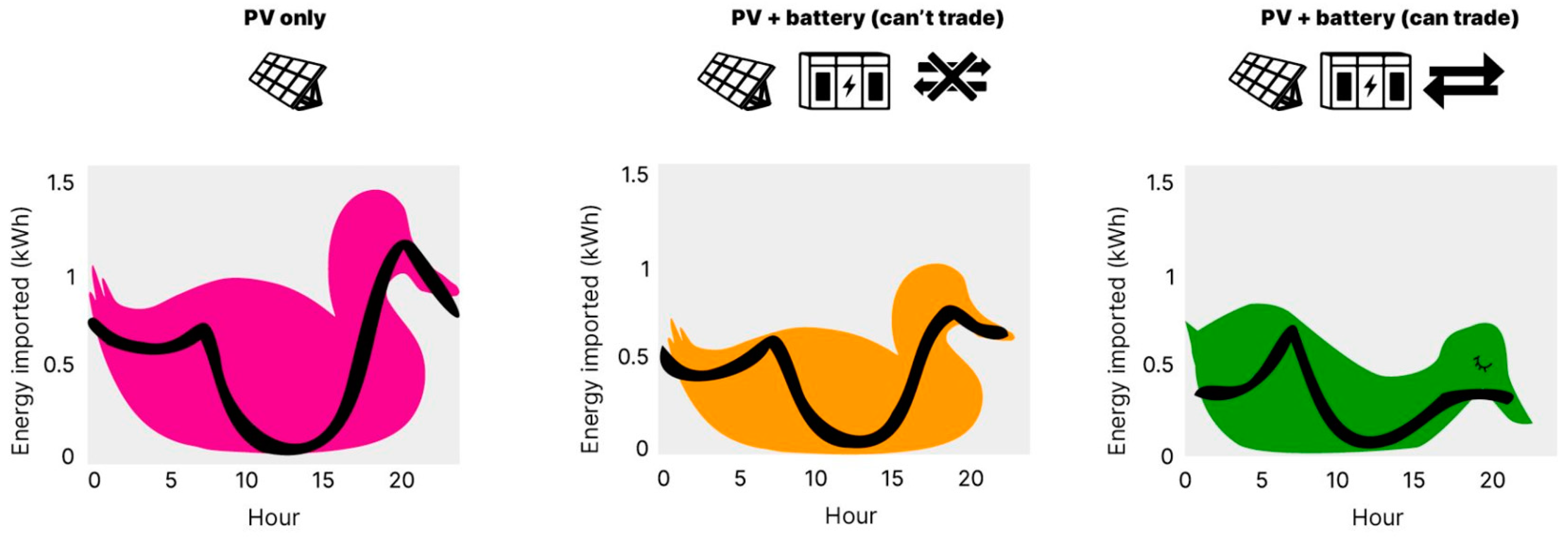
As can be seen, the midday solar saturation and evening ramp, also known as the “belly” and “neck” of the duck, constitute challenging tasks that require extremely fast ramp rates from the conventional generating units. In addition, increasing the contribution of RES, the spinning reserve capability is decreased, deteriorating the system stability and reliability [22]. To ameliorate for the security-constraint problem of optimal unit commitment and allow for a smoother transition towards carbon-free and environmentally friendly energy resources, electricity storage solutions are continuously assessed in a wide variety of applications. In this way, the current thermal resources can be replaced with future low-carbon alternatives which will be quite ‘dispatchable’. However, this solution adds considerable uncertainty and cost, while the residual load for the conventional generators may fluctuate even more stochastically. Figure 2 illustrates three typical paradigms without storage, in the presence of storage, and with prosumer participation.

2.2. Wind Generation

Wind turbines can convert the kinetic energy from wind to electrical energy with the aid of rotor blades based on the following equation.

$$P_w={\displaystyle \frac{1}{2}}·{\rho }_{air}·A·v_w^3$$

(4)

P_w constitutes the wind power as a function of the air density (ρ_air), the spanned area by the rotor blades (A), and the wind velocity (v_w). However, a turbine cannot extract 100% of the kinetic energy from wind according to the Betz limit (c_p ~ 59.26%). In this way, the maximum power output from a wind turbine can be obtained via Equation (5).

$$P_w={\displaystyle \frac{1}{2}}·c_P·{\rho }_{air}·A·v_w^3$$

(5)

According to the type and scale of the wind turbine, most manufacturers define the kinetic energy converted into electricity as a function of the rated power P_r and wind speed v_r with respect to the cut-in v_i and cut-out speed v_o speed. In this regard, the following formulation can be used:

$$P_w\left(t\right)=\left\{\begin{array}{ll}{P}_r,& v_r\le v_w\le v_o\\ P_r{\displaystyle \frac{v_w\left(t\right)-v_i}{v_r-v_i}},& v_i<v_w<v_r\\ 0,& v_w\le v_{i}or{v}_w>v_o\end{array}\right.$$

(6)

The wind velocity v_w,ref is measured at weather stations with a pre-defined height h_w,ref (e.g., 10 m), which may be significantly lower than the actual height h_w of a wind turbine (~100 m). At the desired height, these measurements can be corrected to represent the actual velocity v_w based on Equation (7), combining the roughness of the terrain h_o.

$$v_w=v_{w,ref}·{\displaystyle \frac{\ln \left(\frac{h_w}{h_o}\right)}{\ln \left(\frac{h_{w,ref}}{h_o}\right)}}$$

(7)

Together with wind direction, these parameters are the most important to estimate the actual power output from wind turbines, while pitch regulation, gear selection, and yaw angle control are performed in order to keep c_p near its maximum value considering the tip speed ratio (TSR or λ) as follows:

$$\lambda ={\displaystyle \frac{\omega ·r}{v_w}},$$

(8)

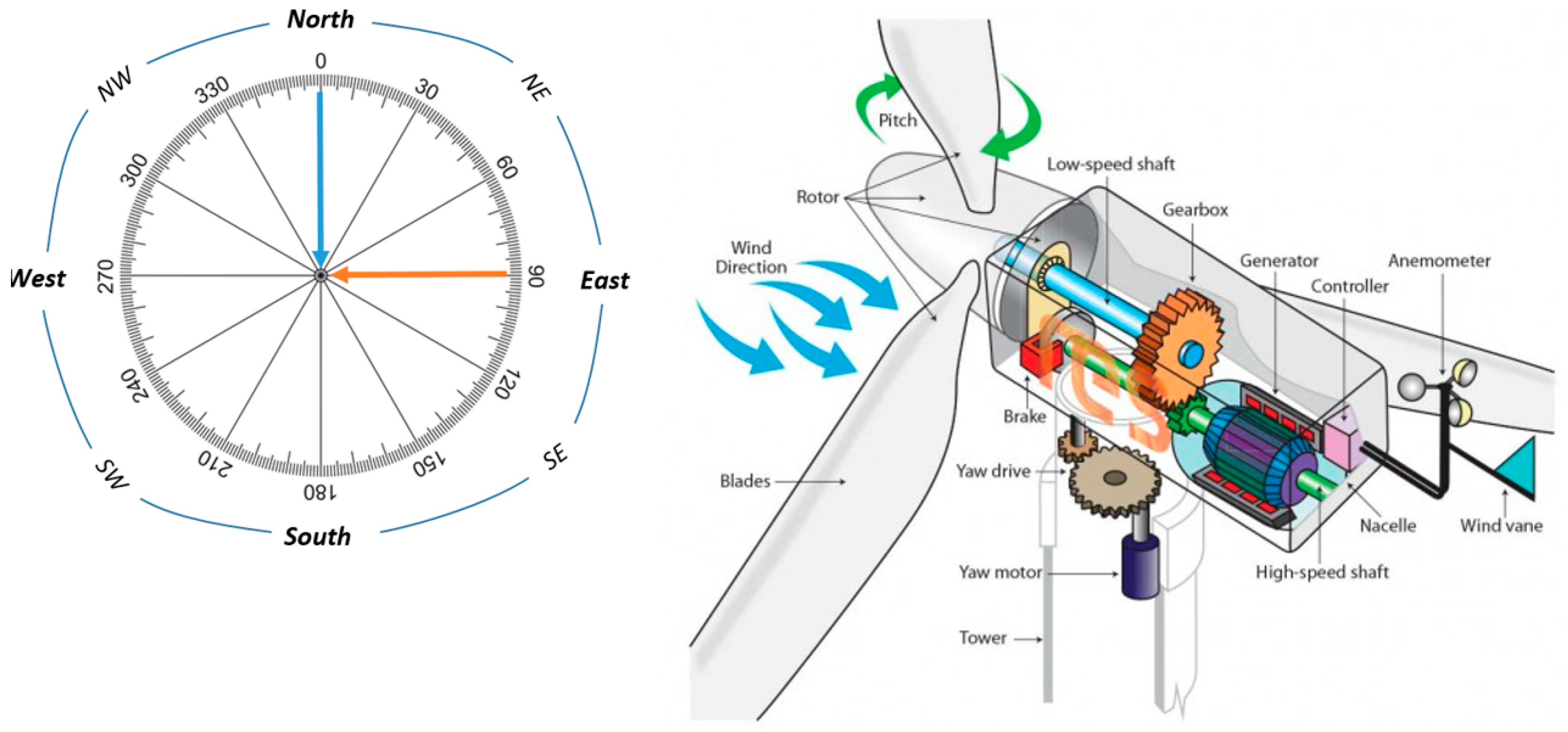
where r is the radius of the circular disc formed by the blades and ω defines the rotational speed. Figure 3 demonstrates a simulation of a wind turbine and a simple diagram for the determination of wind direction in degrees. Identifying the parameters A, h_w, r, c_p and the variables ρ_air, λ, v_w, required to estimate the wind power generation, the necessary data collection can take place as will be explained in the model description section.

Wind power forecasting plays a pivotal role in the efficient integration of renewable energy into the grid. However, several uncertain parameters pose significant challenges to accurate predictions. One of the foremost factors contributing to uncertainty is the variability in wind speed, which is inherently unpredictable and subject to rapid changes. Additionally, the performance and characteristics of wind turbines introduce uncertainties, encompassing factors such as degradation over time and variations in equipment specifications. Meteorological conditions, including temperature, air density, and atmospheric pressure, further compound the intricacies of wind power forecasting. Accurate prediction of wind direction is paramount, as changes in this parameter can markedly impact the performance of wind turbines. Furthermore, the local topography, including hills, valleys, and other geographical features, plays a crucial role in influencing wind patterns, adding another layer of complexity to forecasting models.

Addressing the uncertainties associated with seasonal and diurnal variations is equally imperative for reliable wind power forecasting. Wind patterns exhibit cyclic variations over the course of a day and are subject to seasonal shifts, necessitating robust modeling approaches. Moreover, the quality and availability of data, both historical and real-time, introduce uncertainties into forecasting models. Data gaps, inaccuracies, and limitations in measurement technologies must be carefully considered. Climate change effects on wind resources represent an emerging concern, with potential long-term impacts on forecasting accuracy. The integration of wind power into the grid is also contingent on understanding and mitigating uncertainties related to transmission and grid constraints. Finally, the parameters within the forecasting models themselves, such as algorithm selection, time horizons, and updating frequencies, contribute to the overall uncertainty in wind power forecasting.

2.3. PV Generation

Electric power can be provided directly from solar PV panels considering the photovoltaic conversion efficiency (η_pv), the global solar irradiation (G_A), and the ambient temperature (T_a). According to the type of the PV arrays employed, some technical parameters are also needed to estimate the actual power output. These refer to the solar radiation under standard conditions (G_SC), the temperature under standard conditions (T_SC), and the PV temperature coefficient (C_T). Hence, a nominal output (P_SC) under 25 °C and 1 kW/m², which are usually taken into account by manufacturers during testing and validation, is given and the actual PV generation (P_pv) is estimated as:

$$P_{PV}=P_{SC}·{\eta }_{PV}·{\displaystyle \frac{G_A}{G_{SC}}}·\left[1+\left(T_a-T_{SC}\right)·C_T\right]$$

(9)

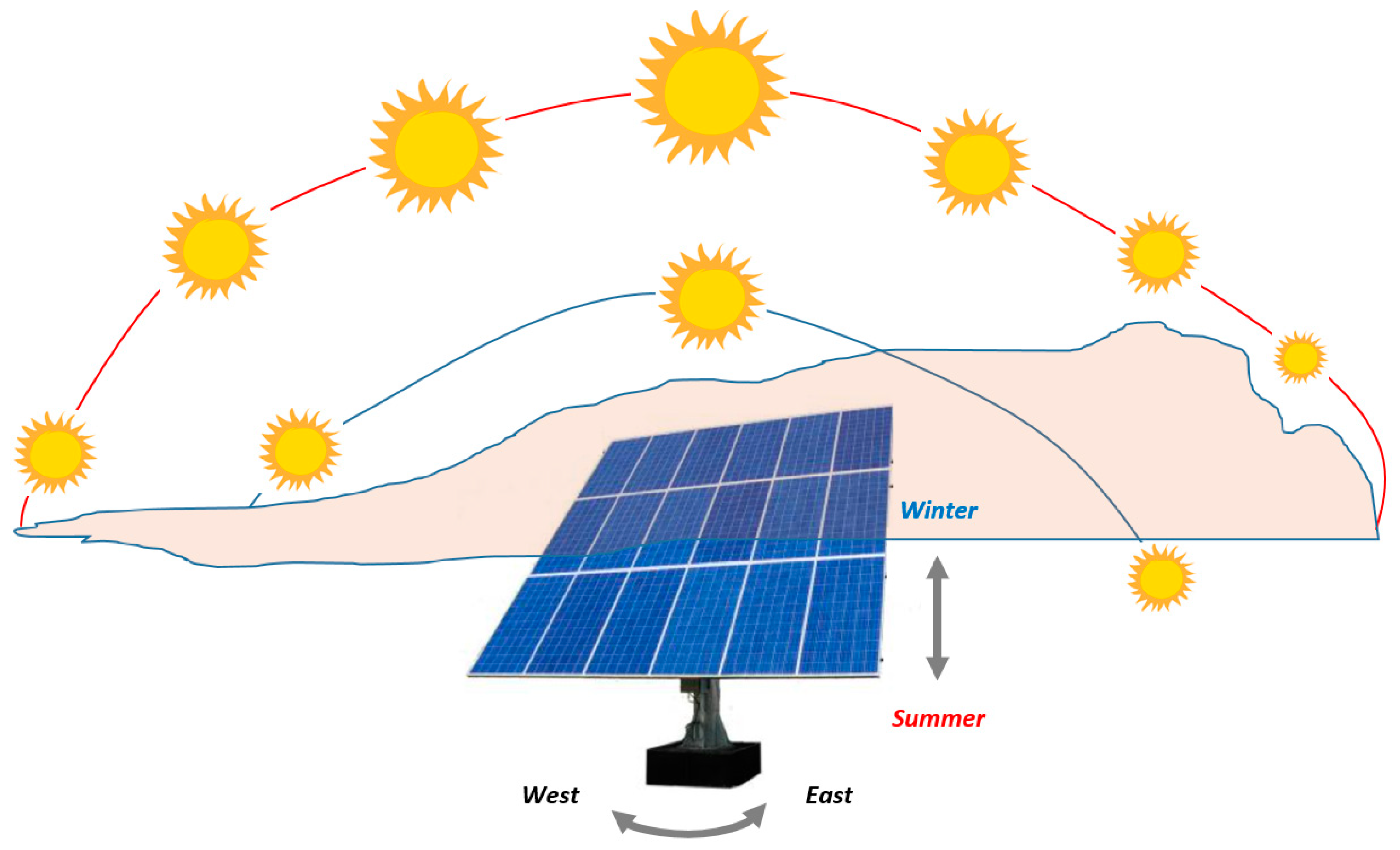
Tilted PV modules show an angular loss due to the fact that the irradiation is not always perpendicular to the PV surface during the day and the year. Therefore, two tilt- angle corrections can be made via two-axis tracking systems, namely the module tilt angle from vertical axis a and the tilt angle from horizontal axis β. During daylight (from sunrise to sunset), β can vary from 0° to 180°, tracking the sun’s direction from east to west. During the year, and according to the season, a ranges between 0° and 90° to increase the solar absorption towards maximum conversion efficiency [23]. Figure 4 illustrates a paradigm of a PV module with a two-axes tracking system.

G_A can vary depending on the cloud cover prevailing at a given time. Thus, a clearness index indicating the fraction of solar radiation transmitted through the atmosphere to strike the earth’s surface can be used. Utilizing a dimensionless number between 0 and 1, it can range between a minimum of 0.25 and the maximum of 0.75, to define a mostly cloudy and a mostly sunny day, respectively. A similar effect can be observed with dust and other atmospheric particulate matter (PM) which is able to reduce the solar energy provision by ~17–25% with roughly equal contributions from ambient PM and PM deposited on photovoltaic surfaces [24].

Finally, the impact of temperature on a PV panel must be considered. The controversial effect of decreased generation during higher solar irradiance can be explained by engaging the ambient temperature information. According to Equation (9), every 1 °C above the standard temperature of 25 °C can decrease the photovoltaic efficiency by 0.3–0.5% (assuming that the temperature coefficient sits between −0.3 and −0.5%/°C).

Accurate forecasting of solar photovoltaic power output is essential for the effective integration of renewable energy into the grid. However, numerous uncertain parameters contribute to the complexity of predicting solar PV generation. Central among these is the variability in solar irradiance, influenced by dynamic atmospheric conditions, cloud cover, and diurnal cycles [25,26]. Addressing this uncertainty is paramount for reliable predictions, as fluctuations in irradiance directly impact the energy yield of solar panels. Additionally, the effects of temperature on PV panel performance introduce a layer of unpredictability, requiring sophisticated modelling to capture temperature-related efficiency changes accurately. Beyond these meteorological factors, considerations of panel soiling and degradation over time become integral, affecting the long-term reliability of PV systems. The challenge extends further to encompass shadowing and obstructions, as well as the optimal orientation and tilt angles of solar panels, which collectively influence the spatial and temporal distribution of sunlight exposure.

Inverter efficiency represents another critical parameter introducing uncertainty into solar PV power predictions. Accurate conversion of direct current (DC) to alternating current (AC) is pivotal for maximizing energy output, and fluctuations in inverter efficiency must be meticulously considered. Moreover, the impact of weather-related factors, such as atmospheric pressure, humidity, and wind speed, on PV performance necessitates a comprehensive approach to forecasting. The quality and availability of data, spanning historical solar irradiance records to real-time measurements, constitute additional sources of uncertainty that researchers must contend with in the development of robust forecasting models. As we strive for greater reliance on solar energy, understanding and mitigating these uncertain parameters are fundamental to advancing the precision and reliability of solar PV power predictions.

3. Model Description

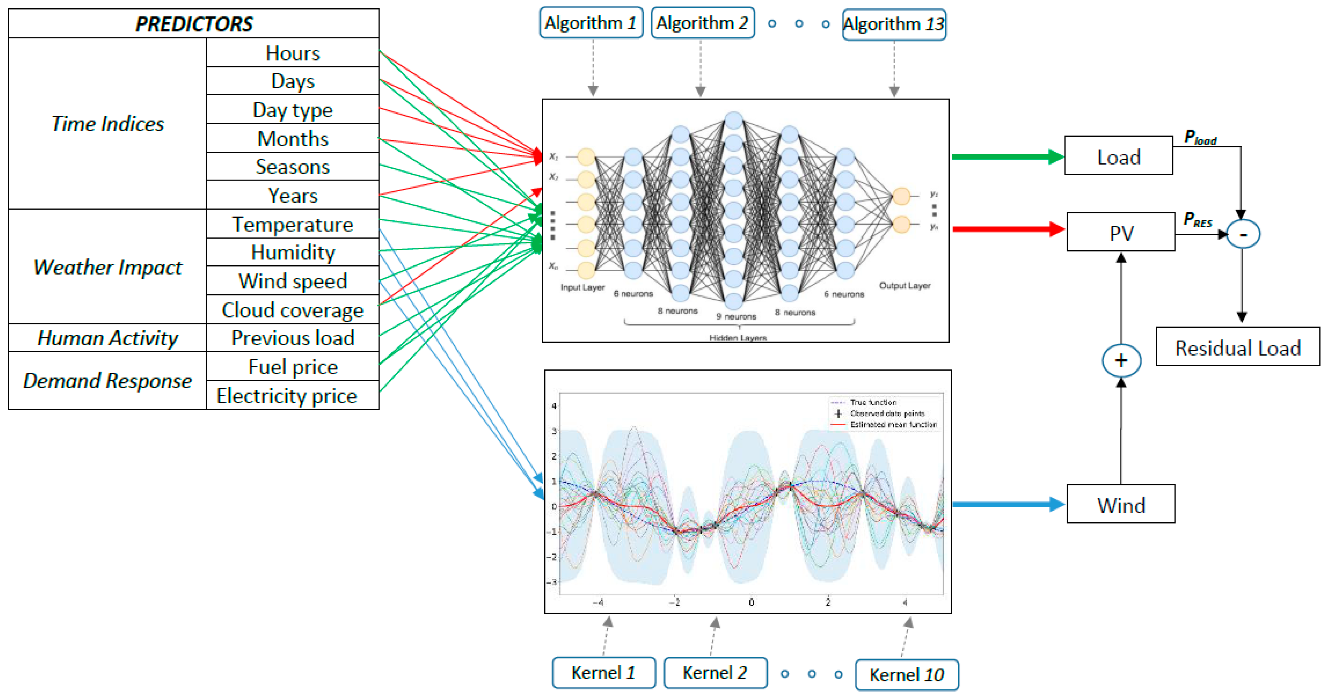
In this section, the proposed model for day-ahead residual load forecasting is described. The input parameters used as predictors are explained in detail along with the mapping process for the relationship between the input predictors and output targets. The generic input factors are classified in five major categories. Constant values such as the Boltzmann constant, Betz limit, water density, and various test conditions are excluded from the studied predictor list. The input parameters including wind turbine heights, fixed tilt angles of PV surface, device efficiency, and so on are also excluded. Although they possess diverse values for each independent system, in total evaluation they occur as constants or target (output) independent variables. The third class regards the controllable variables like tilted PV arrays with tracking systems, pitch and yaw angle, gear ratio, etc. These variables vary towards optimum power output, and thus they are also excluded from the predictor matrix. Following are the non-controllable variables, which are strictly correlated with output target values. These relate the ambient temperature, humidity, cloud coverage, wind speed, energy prices, and past knowledge with respect to the considered targets. Together with the last category, which accommodates the time indices (hour, day, month, season, and year), all uncontrollable variables are used as predictors for the proposed forecasting model.

Aiming at the effective forecast of residual load, the impact of weather is taken into account for the determination of power generation from RES (wind and PV). Wind output is strictly correlated with wind speed, wind direction, and air density. To guarantee that the wind blows perpendicular to the turbine blades, the gear selection process takes place and is not required to be included as a predictor input. On the other hand, the air density formed by controllable and uncontrollable weather variables is indirectly included together with wind speed. Analysing the origin of density, one can simply conclude that it depends on altitude, which forms a parameter, and temperature and humidity which are uncontrollable variables and must be taken into account. On the contrary, PV offers periodically equivalent outputs due to the sun’s position during identical daily, monthly, and seasonal intervals.

With respect to the load demand, the human activity in terms of day type in combination with past load observations, the weather impact, seasonality, and energy price are considered as important predictors for a proper day-ahead prognostication. Consequently, the required predictors, for which historical data must be obtained, are day type, temperature, humidity, wind speed, cloud coverage index, fuel price, electricity price, previous-day load, previous-week load, and previous-year load. These are related to the output targets f load demand, wind, and solar PV output and are grouped by hour of day, day of the year, the month, the season, and the year. It is worth noting that, apart from the knowledge of the previous load, the rest of the inputs constitute forecasted values for the day-ahead representation.

Table 1. Predictors and targets required for training the proposed model.

Predictors		Targets
Indices	Variables	Residual Load
Hours	Temperature	Load
Days	Humidity
Day type	Wind speed	Wind
Months	Cloud coverage
Seasons	Energy price	PV
Years	Previous load

lists the selected predictors and targets by category.

Hours and days form important predictors in predicting the PV output. In normal cases, the cloud coverage index may help the model to increase the accuracy; more enhanced configurations must involve the temperature, humidity, and years. Apart from the weather impact, the input indicating the year under assessment provides the information of PV installations added from year to year (translated as capacity increments). To forecast the fluctuating load in enhanced systems, all time indices are needed (hours, days, day types, months, seasons, and years) along with the weather impact predictors of temperature, humidity, and cloud coverage. In addition, the load trend can be explained via the previous load knowledge, and overall customer behavior is affected by the varying energy prices. The last target, wind power, is time-independent and is affected only by wind speed and air density, which can be defined equivalently by the ambient temperature and relative humidity.

Neural networks are often preferred for load forecasting due to their ability to model complex, nonlinear relationships between input variables and the target output, which is particularly useful in capturing the intricate dynamics of energy demand. They can effectively learn from historical data and identify patterns that traditional statistical methods might miss. Additionally, neural networks are highly flexible and can be adapted to different forecasting horizons (short-, medium-, or long-term) and can handle large amounts of data, improving the accuracy and robustness of predictions. Their capability to generalize well across varying conditions makes them ideal for dealing with the uncertainties and fluctuations in load forecasting. The developed model exploits a feed-forward neural network with a varying number of hidden layers. The layers vary from one to five according to the number of input predictors under assessment. In more detail, a number (K) of predictors x are imported in the feed-forward network along with the target y to form the dataset $\left.x_i,y_i\right|i=1,\dots ,n$. The model is trained using the largest share (70%) of the historical data for training, while the rest is equally distributed for validation (15%) and testing (15%). The multi-input/multi-output model is employed as follows [27]. Considering six neurons for the first hidden layer (h₁₁–h₁₆), Equations (10) and (11) can be employed to extract the first output h₂₁.

$$h_{11}=\sigma \left(\sum _{k=1}^K{w}_k{x}_k+b_{11}\right)$$

(10)

$$h_{21}=\sigma \left(\sum _{k=1}^6{w}_k{h}_{1_k}+b_{21}\right)$$

(11)

This is repeated through the neural configuration [6, 8, 9, 8, 6] for the respective five hidden layers, estimating the outputs of h₂₁–h₂₈, h₃₁–h₃₉, h₄₁–h₄₈, h₅₁–h₅₆ and the final target of y (Equations (12)–(16)).

$$h_{38}=\sigma \left(\sum _{k=1}^6{w}_k{h}_{2_k}+b_{38}\right)$$

(12)

$$h_{49}=\sigma \left(\sum _{k=1}^8{w}_k{h}_{3_k}+b_{49}\right)$$

(13)

$$h_{58}=\sigma \left(\sum _{k=1}^9{w}_k{h}_{4_k}+b_{58}\right)$$

(14)

$$h_{66}=\sigma \left(\sum _{k=1}^8{w}_k{h}_{5_k}+b_{66}\right)$$

(15)

$$y=\sum _{k=1}^6{w}_k{h}_{6_k}+b_y$$

(16)

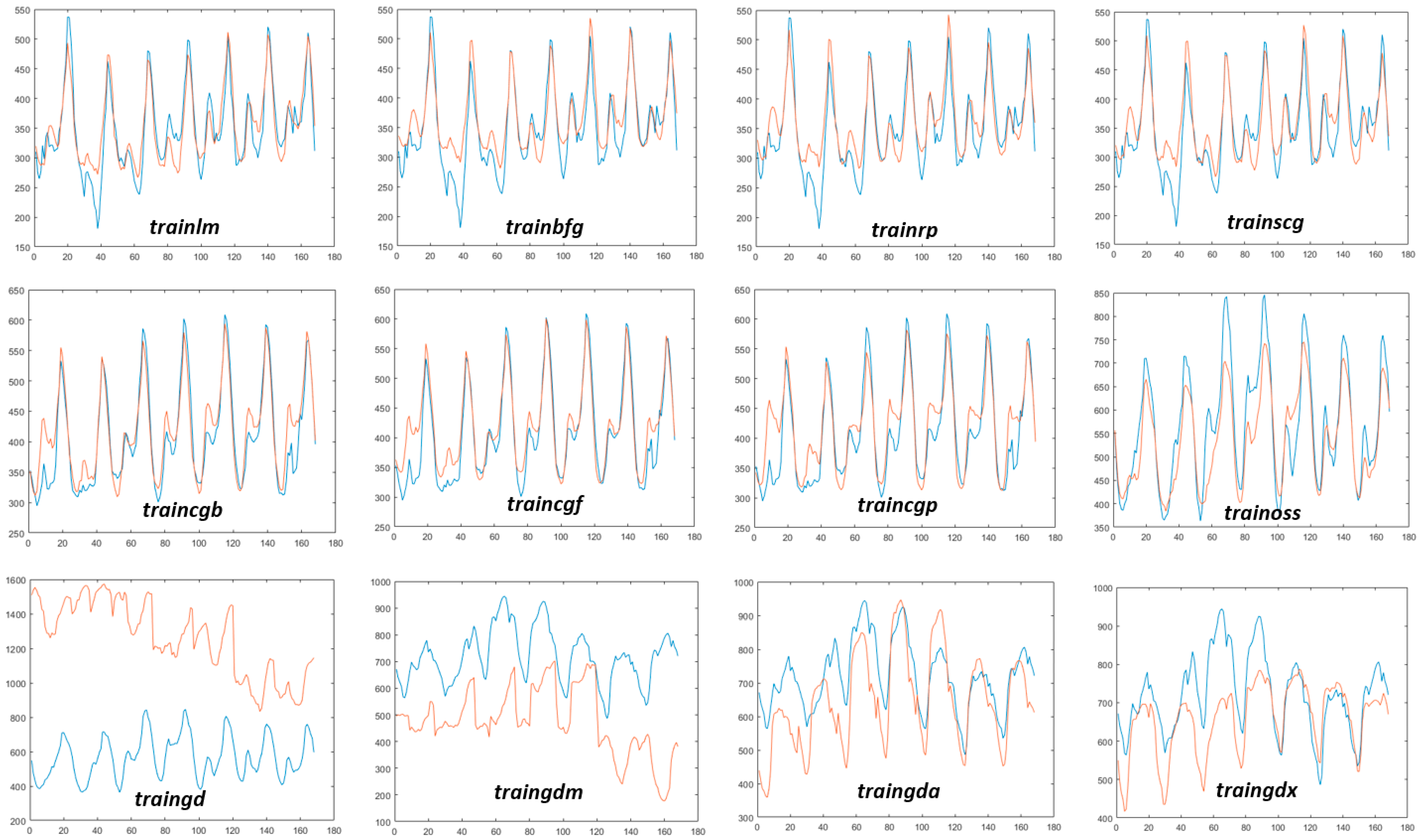
The sigmoid activation function is expressed via σ(.), h_i is the output of each hidden layer, w_k constitutes the weights, and b_i represents the bias operator. A temporal optimal observation y at each iteration k is assumed as target data, and the scope is to effectively reduce the error between this target outcome and the progressively obtained pattern solution. To this end, different algorithms can be used to update the weight matrix and bias between consecutive iterations (e.g., k and k + 1). For example, performing simulations in MATLAB R2022-MathWorks, the available training algorithms (and their respective function) for nonlinear regression are: Levenberg Marquardt (trainlm), BFGS Quasi-Newton (trainbfg), resilient backpropagation (trainrp), scaled conjugate Gradient (trainscg), conjugate gradient with Powell/Beale restarts (traincgb), Fletcher-Power conjugate gradient (traincgf), Polak-Ribiere conjugate gradient (traincgp), one-step secant (trainoss), Bayesian regularization (trainbr), gradient descent (traingd), gradient descent with momentum backpropagation (traingdm), gradient descent adaptive learning rate backpropagation (traingda), gradient descent with momentum, and adaptive learning backpropagation (traingdx).

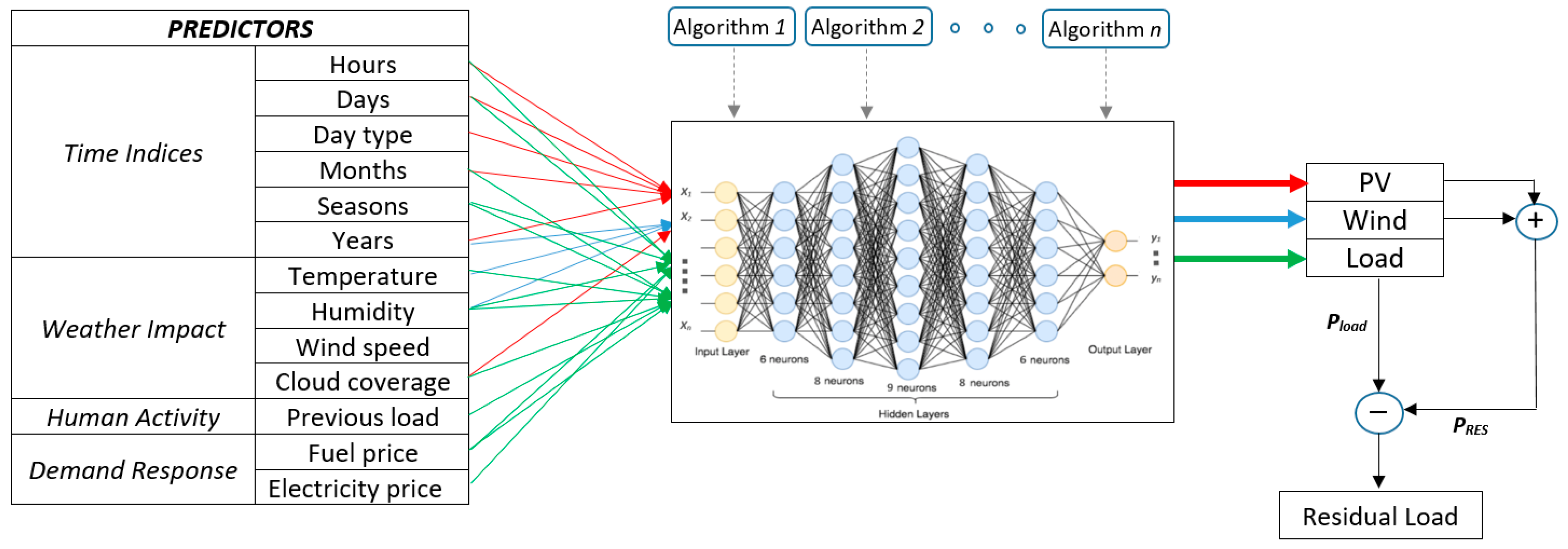
In this way, the neural is separately used to make use of an algorithm at a time and to observe the targets of load, PV, and wind power, while the residual load is estimated by the model based on Equation (3). Figure 5 depicts the proposed multi-input/multi-output model. Time series data with hourly resolution are used as input predictors. To distinguish the targets, all data are separated by hours, days, day types, months, seasons, and years, each one forming an individual input. Hence, the inputs of temperature, humidity, wind speed, cloud coverage, energy price, and previous load constitute Mx1 vectors, where M equals to 26,280 (assuming 3 years, 365 days/year, and 24 h/day).

Utilizing one of the aforementioned training algorithms each time, a neural network with different inputs is employed for every target. Based on this model, the prediction is performed using 24 h forecasted values recording the output. Once the day-ahead forecast of load demand, PV, and wind output is completed, the residual load is estimated and the performance metrics are recorded. The procedure is repeated for the 13 training algorithms. To account for the imposed uncertainty between the actual and predicted residual load, nonparametric models can take place. Gaussian process regression (GPR) is expected to be favored for load forecasting because of its ability to provide not only accurate predictions but also a measure of uncertainty in those predictions, which is crucial for managing energy systems. It also performs well with small- to medium-sized datasets, as it does not require large amounts of data to achieve high accuracy. GPR models are nonparametric, probabilistic models that rely on kernel functions. Considering a training set $\left\{\left(x_i,y_i\right);i=\mathrm{1,2},\dots ,n\right\}$ where $x_i\in {\mathbb{R}}^d$ and $y_i\in {\mathbb{R}}^d$ are drawn from an unknown distribution, the goal of a GPR model is to predict the response variable y_new, given the new input vector x_new, and the information from the training data. A linear regression model is expressed as:

$$y=x^T\beta +\epsilon ,$$

(17)

where $\epsilon ~\mathsf{{\rm N}}\left(0,{\sigma }^2\right)$. The error variance ${\sigma }^2$ and the coefficients β are typically estimated from the data. A GPR model explains the response by introducing latent variables, $f\left(x_i\right),i-\mathrm{1,2},\dots ,n$, derived from a Gaussian process, along with explicit basis functions, h. The covariance function of these latent variables reflects the smoothness of the response, while the basis functions map the inputs x to a p-dimensional feature space. Gaussian process is a collection of random variables, such that any finite subset has a joint Gaussian distribution. Therefore, if we define $\left\{f\left(x\right),x\in {\mathbb{R}}^d\right\}$ as a Gaussian process, then for given observations $x_1,x_2,\dots ,x_n$, the random variables $f\left(x_1\right),f\left(x_2\right),\dots ,f\left(x_n\right)$ follow a joint Gaussian distribution. To comprehensively specify it, the mean value is defined via the function m(x), whereas the covariance is demonstrated by $k\left(x,x^{\prime }\right)$. Specifically, if $\left\{f\left(x\right),x\in {\mathbb{R}}^d\right\}$ forms a GP, then $E(f\left(x\right)=m(x)$ and $Cov\left[f\left(x\right),f\left(x^{\prime }\right)\right]=E\left[\left\{f\left(x\right)-m\left(x\right)\right\}\left\{f\left(x^{\prime }\right)-m\left(x^{\prime }\right)\right\}\right]=k\left(x,x^{\prime }\right)$.

Consider the model ${h\left(x\right)}^T\beta +f\left(x\right)$ where $f\left(x\right)~GP(0,k\left(x,x^{\prime }\right))$. This represents a GPR framework, where the response variable can be modelled as:

$$P\left(y|f,X\right)~N\left(y_i|{h\left(x_i\right)}^T\beta +f\left(x_i\right),{\sigma }^2\right)$$

(18)

For each observation x_i, the joint distribution of latent variables $f\left(x_1\right),f\left(x_2\right),\dots ,f\left(x_n\right)$ is presented in vector form as $P\left(f|X\right)~N\left(f|0,K(X,X)\right)$, where $K(X,X)$ is written as follows:

$$K\left(X,X\right)=\left(\begin{array}{ccc}\begin{array}{c}k\left(x_1,x_1\right)k(x_1,x_2)\\ k\left(x_2,x_1\right)k(x_2,x_2)\end{array}& \cdots & \begin{array}{c}k(x_1,x_n)\\ k(x_2,x_n)\end{array}\\ ⋮& \ddots & ⋮\\ k\left(x_n,x_1\right)k(x_n,x_2)& \cdots & k(x_n,x_n)\end{array}\right)$$

(19)

The covariance function $k\left(x,x^{\prime }\right)$ is typically parameterized by a set of kernel parameters or hyperparameters, denoted by θ. Sometimes, $k\left(x,x^{\prime }|\theta \right)$ is used to explicitly show this dependence on θ. Exploiting a fitness function available in MATLAB R2022, known as ‘fitrgp’, the kernel values of β, σ² and θ can be estimated during the training of the GPR model. Hence, the covariance (or kernel) function expresses how the response (or target) y_i at one point x_i is affected by responses (y_j) at other points x_j which possess similar predictor values. The characteristic length, σ_l, is utilized to define a magnitude apart from which the input values are treated as uncorrelated to the response output.

During the evaluation of the demonstrated MIMO using GPR, two categories of kernel functions have been tested. The first category pertains to the exponential, the squared exponential, the Matern 3/2, the Matern 5/2, and the rational quadratic kernel functions which concern same length-scale for each predictor. The other category accommodates the built-in functions which consider a separate length scale for each predictor. These kernels are referred to as automatic relevance determination (ARD) alternatives. The mathematical expressions of the kernel functions used are listed in

Table 2. Mathematical formulation of the assessed kernel functions.

Kernel Function	Formulation	Euclidian Distance
Exponential	$k\left(x_i,x_j|\theta \right)={\sigma }^{2}exp\left(-{\displaystyle \frac{r}{{\sigma }_l}}\right)$	$r=\sqrt{{\left(x_i-x_j\right)}^T\left(x_i-x_j\right)}$
Squared Exponential	$k\left(x_i,x_j|\theta \right)={\sigma }^{2}exp\left(-{\displaystyle \frac{r^2}{2{\sigma }_l}}\right)$
Matern 3/2	$k\left(x_i,x_j|\theta \right)={\sigma }^2\left(1+{\displaystyle \frac{\sqrt{3}r}{{\sigma }_l}}\right)exp\left(-{\displaystyle \frac{\sqrt{3}r}{{\sigma }_l}}\right)$
Matern 5/2	$k\left(x_i,x_j|\theta \right)={\sigma }^2\left(1+{\displaystyle \frac{\sqrt{5}r}{{\sigma }_l}}+{\displaystyle \frac{\sqrt{5}{r}^2}{3{{\sigma }_l}^2}}\right)exp\left(-{\displaystyle \frac{\sqrt{5}r}{{\sigma }_l}}\right)$
Rational Quadratic *	$k\left(x_i,x_j|\theta \right)={\sigma }^2{\left(1+{\displaystyle \frac{r^2}{2a{{\sigma }_l}^2}}\right)}^{-a}$
ARD Exponential	$k\left(x_i,x_j|\theta \right)={\sigma }^{2}exp\left(-r\right)$	$r=\sqrt{{\displaystyle \sum _{m=1}^d}{\displaystyle \frac{{\left(x_{im}-x_{jm}\right)}^2}{{\sigma }^2}}}$
ARD Squared Exponential	$k\left(x_i,x_j|\theta \right)={\sigma }^{2}exp\left(-{\displaystyle \frac{r^2}{2}}\right)$
ARD Matern 3/2	$k\left(x_i,x_j|\theta \right)={\sigma }^2\left(1+\sqrt{3}r\right)exp\left(-\sqrt{3}r\right)$
ARD Matern 5/2	$k\left(x_i,x_j|\theta \right)={\sigma }^2\left(1+\sqrt{5}r+{\displaystyle \frac{5}{3}}{r}^2\right)exp\left(-\sqrt{5}r\right)$
ARD Rational Quadratic *	$k\left(x_i,x_j|\theta \right)={\sigma }^2{\left(1+{\displaystyle \frac{r^2}{2a}}\right)}^{-a}$

* α represents a positive scale-mixture parameter.

. The Euclidian distance between x_i and x_j is noted by r, while θ expresses the vector of ${\theta }_1=log{\sigma }_l$ and ${\theta }_2=log\sigma$, which forces both σ_l and σ to be always a positive number.

4. Experimental Evaluation

Considering different algorithms for training purposes and a deep neural network with five hidden layers, the proposed MIMO model is assessed under three case studies based on real historical data from 2018 to 2022. A second experiment takes place to compare the ANN with GPR under the exploitation of different kernel types. The assessed system regards the isolated power system of the island of Cyprus. As the third-largest and third-most-populous island in the Mediterranean, Cyprus constitutes a representative islanded system within Europe, lying between 34° and 36° N latitudes and 32° and 35° E longitudes. The ~1.1 million inhabitants are distributed, by ranking, in the cities of Nicosia (Capital), Limassol, Larnaca, and Paphos, composing a density of about 123.4/km². Up to the end of the 2020s, the island’s electricity needs were satisfied mostly by making use of imported conventional fuels (heavy fuel oil and diesel) via three power plants at a rate close to 85% [28]. The rest was supplied by domestic renewable energy sources, including biomass, wind, and solar PV systems. However, biomass has been excluded from the forecasting task since it constitutes a storable energy carrier with predictable and simply controllable potential. The actual data pertaining to the PV and wind power generated across the real load demand and weather conditions were obtained from the Cyprus energy regulatory authority (CERA). To avoid any distortion, extreme values have been identified using a simple outlier detection method and replaced by their mean consecutive values. Then, a cross-validation process took place considering the capacity expansions per month, in order to maintain data integrity, accuracy, and reliability throughout the historical data.

4.1. Input Profile

To justify the selection of the most relevant input features, both the Pearson method and mutual information are employed. The Pearson method is used to estimate the correlation coefficients and the mutual dependency between the input features and wind power output. Considering the input variables x_i, the output Y_i, and their respective mean values $\overline{x}$ and $\overline{Y}$, the correlation coefficient $r\in [-1,+1]$ is defined as [29]:

$$r={\displaystyle \frac{\sum \left(x_i-\overline{x}\right)\left(Y_i-\overline{Y}\right)}{\sqrt{\sum {\left(x_i-\overline{x}\right)}^2{\left(Y_i-\overline{Y}\right)}^2}}}$$

(20)

By treating the predictor/target pairs as random variables X and Y, their mutual dependencies can be quantified using Equation (21) [30]. This approach considers the number of respective states, S_n and S_m, along with their joint probability P(x_n, Y_m) and marginal probabilities P(x_n) and P(Y_m). The mutual information $I\in [0,+\infty )$ is then computed as follows:

$$I\left(X;Y\right)=\sum _{n=1}^{S_n}\sum _{m=1}^{S_m}P\left(x_n,Y_m\right)\log {\displaystyle \frac{P\left(x_n,Y_m\right)}{P\left(x_n\right)P\left(Y_m\right)}}$$

(21)

Among the input features, the predictors that demonstrate the highest correlation (r ≥ 0.20) and dependency (I ≥ 0.25) with their respective target were included in the first case study. As previously mentioned, the factors involved in estimating load and generation are distinguished into constants, parameters, controllable variables, uncontrollable variables, and indices. Assuming that $P_{RL}=P_{load}-P_{wind}-P_{pv}$, and expressing each component of the right side of the equation in terms of the uncontrollable variables, the necessary elements for which we need historical data collection can appear. In this way, the uncontrollable variables of temperature, humidity, and fuel cost (c_f) are consolidated as:

$$P_{load}=f\left(T,H,c_f\right)$$

(22)

If information from past load facts (indicated with apostrophes such as: $P_{load}^{\prime }$ for the previous day load, $P_{load}^{″}$ for the previous week load, and $P_{load}^{‴}$ for the previous year load) are taken into account, (17) can be rewritten as presented below. The mathematical representation of load parameters is respectively indicated as $P_{load}^{\prime }\left(t\right)=P_{load}(t-24)$, $P_{load}^{″}\left(t\right)=P_{load}(t-168)$ and $P_{load}^{‴}=P_{load}(t-8760)$. In Equation (18), $c_{el}^{\prime }$ defines the electricity cost, while D determines the day type. Thus, weekdays are indicated with the value “1”, weekends with “2”, and holidays with “3”. While c_f follows the trend of changing crude-oil costs, $c_{el}^{\prime }$ is employed based on peak and off-peak hours during weekdays and weekends, according to

Table 3. Monthly residential and commercial use tariff in cent per unit kWh.

Periods	October–May		June–September
	Weekdays	Weekends/Holidays	Weekdays	Weekends/Holidays
Peak	11.95	11.62	16.74	11.76
Off-peak	10.92	10.57	11.59	11.39

.

$$P_{load}=f\left(T,H,c_f,c_{el}^{\prime },P_{load}^{\prime },P_{load}^{″},P_{load}^{‴},D\right)$$

(23)

In terms of PVs, the indices alone occur adequate at the first step, since the sun’s position is exactly the same comparing identical time intervals within different years. However, to account for the imposed inefficiencies, the variable temperature, humidity, and cloud-coverage index (C) are included to form Equation (24).

$$P_{pv}=f\left(T,H,C\right)$$

(24)

Finally, understanding the dependency of wind power on v_w and ρ_air (which in turn depends on the altitude parameter and uncontrollable temperature and humidity), the following condition can be fulfilled.

$$P_{wind}=f\left(v_w,T,H\right)$$

(25)

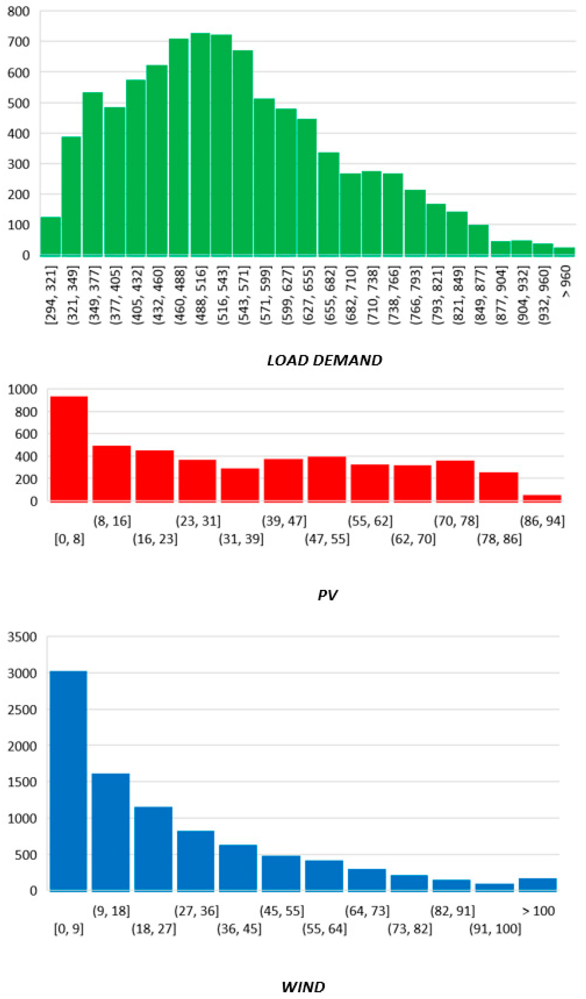
To gain an overview of the system loading, the hourly distribution of MW-power for the annual load and generation is provided in Figure 6. The minimum and maximum needs, the respective contribution of intermittent renewable sources, and their statistical mean, min/max and standard deviation, can be observed in Figure 7.

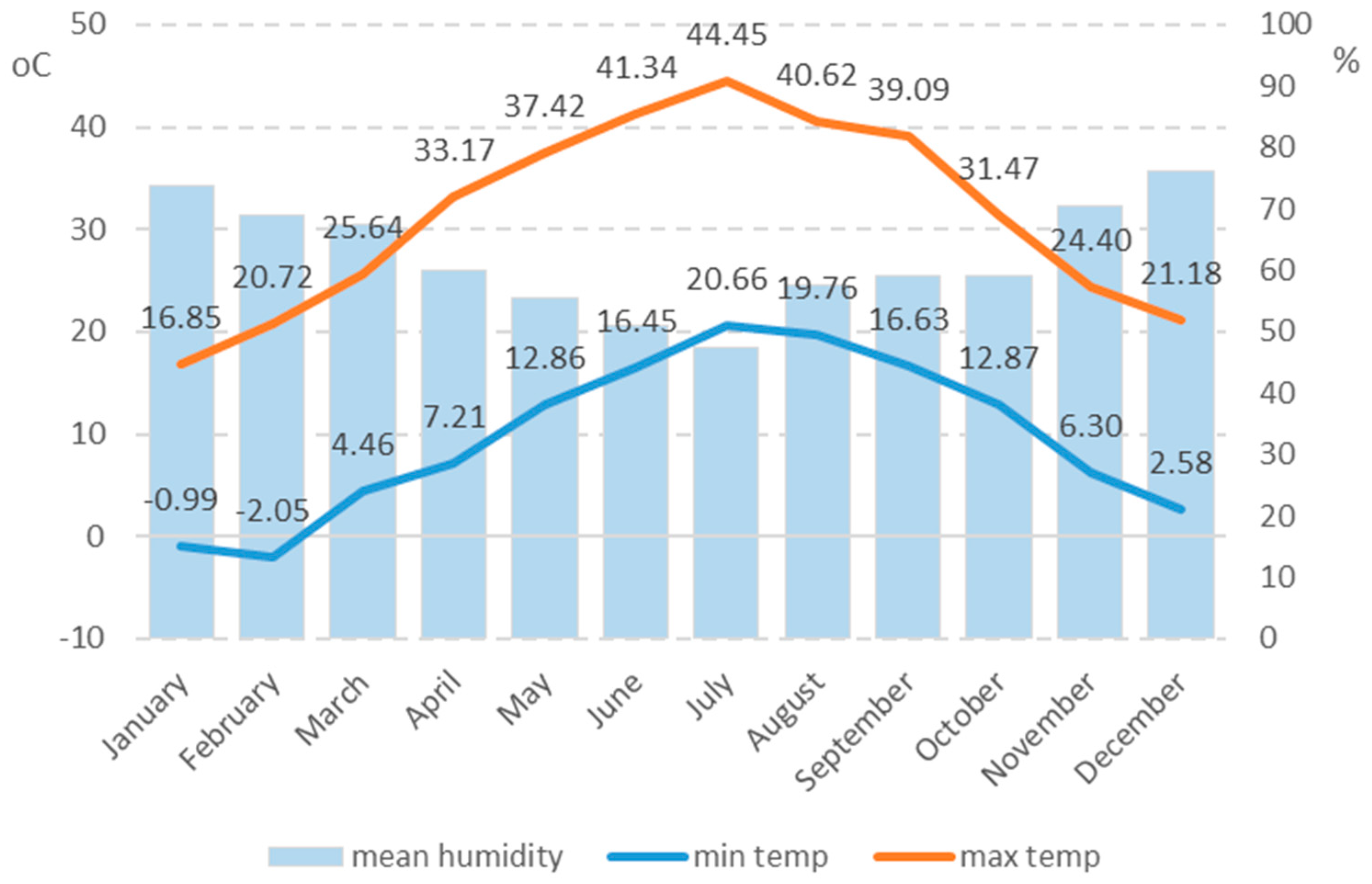
The annual load demand demonstrates a mean of 544 MW, whereas 25 MW and 22 MW are provided by wind farms and PV parks, respectively. During the same year, the temperature showed a big variation between −2.1 °C and 44.5 °C. Its monthly fluctuation can be seen in Figure 8, where the monthly minimum and maximum values are depicted. The average humidity for the respective months is also depicted.

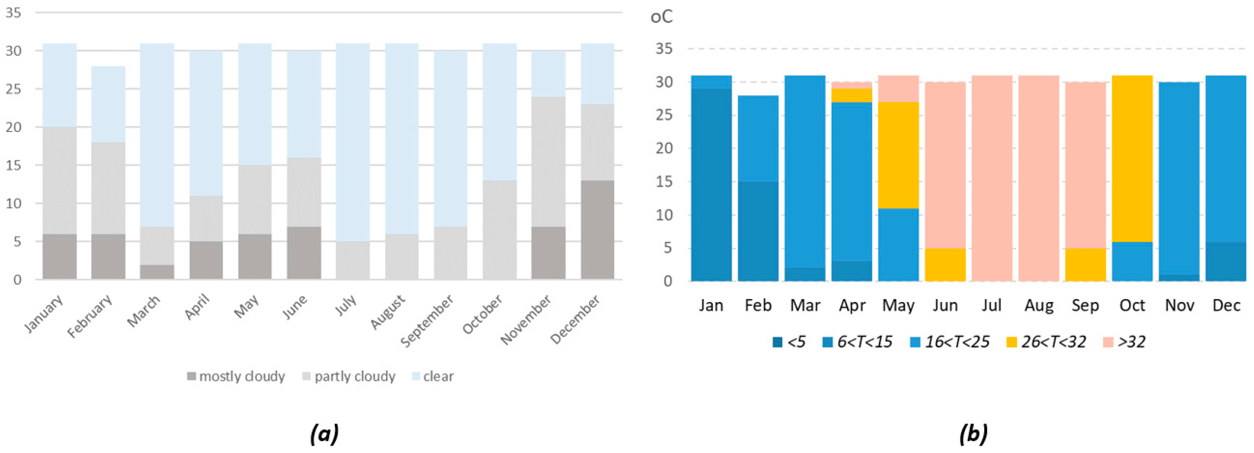
To discuss the correlation of weather conditions with demand and RES production, two monthly histograms are used to represent the cloud coverage and average temperature by month. For this purpose, Figure 9a describes each month in terms of cloudiness. Figure 9b lists the monthly staggered temperature change by counting and distinguishing the days into categories of temperatures below 5 °C (very cold days), within 6 °C and 15 °C (cold days), between 16 °C and 25 °C (normal days), in the range of 26 °C and 32 °C (hot days), and above 32 °C (very hot days).

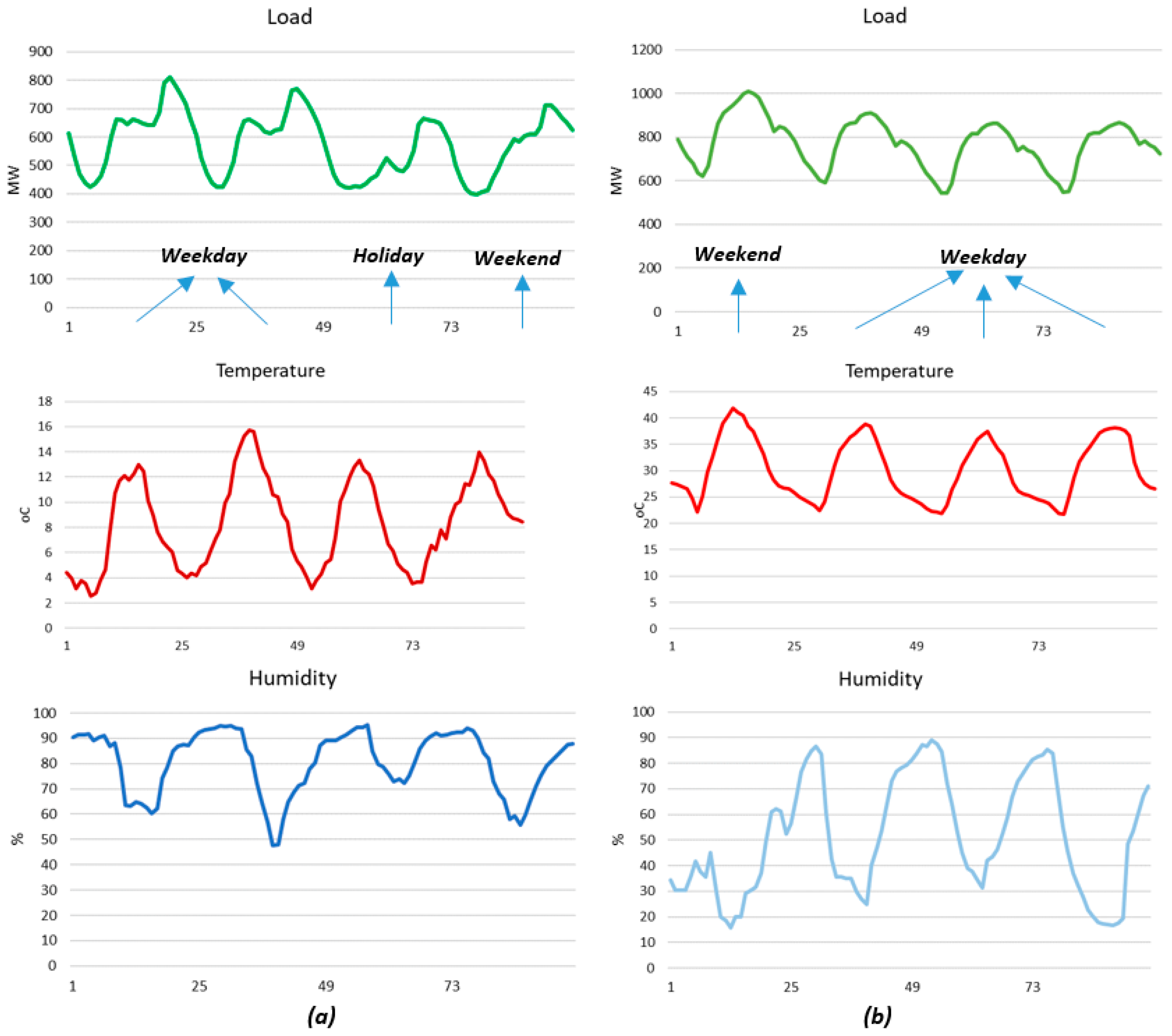
An inversely proportional relation, between load demand and temperature, is illustrated during the winter months. Their relationship becomes proportional during the hotter months in summer, at the beginning of autumn, and at the end of spring. The peak demand coincides with intervals with the highest daily temperature, while in winter, the peak hours are shifted when people return from their work and the ambient temperatures are quite low. As can be seen from Figure 10, higher temperatures during winter allow people to get out and enjoy their holidays and weekends. This results in decreased load demand during daylight.

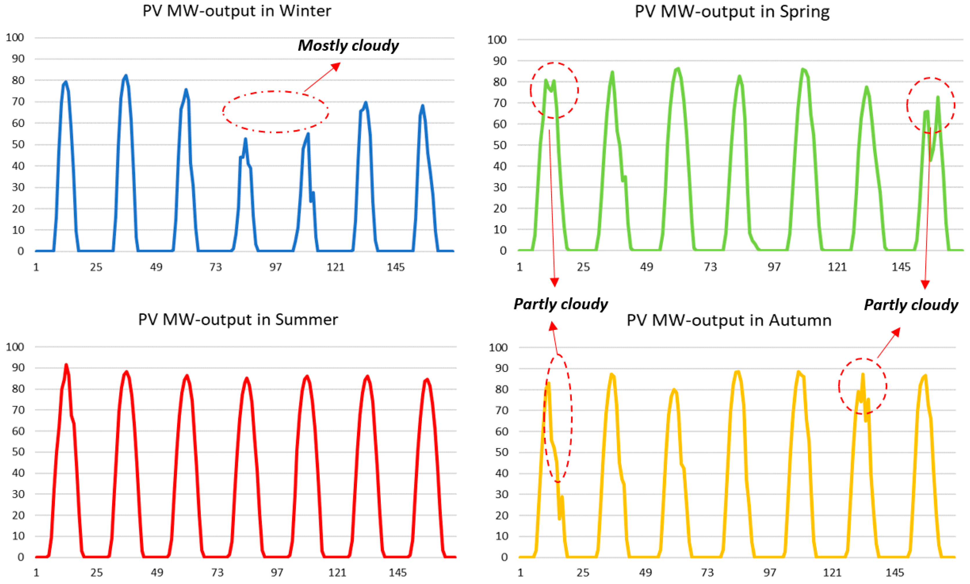
The opposite happens during the same hours in summer, where the higher temperatures, in combination with low humidity, force people to stay home and consume energy for their cooling needs. The respective temperature impact on PV generation shows a slightly negative effect. As can be observed, high temperatures impose efficiency degradation for PVs favoring their contribution during spring and autumn rather than summer. However, due to the enhanced duration between the sunrise and sunset in summer, the total energy PV provision balances these disturbances. Solar radiation possesses the most significant impact on PV generation, and this can be also observed by the cloud coverage index applied during partly cloudy and mostly cloudy days.

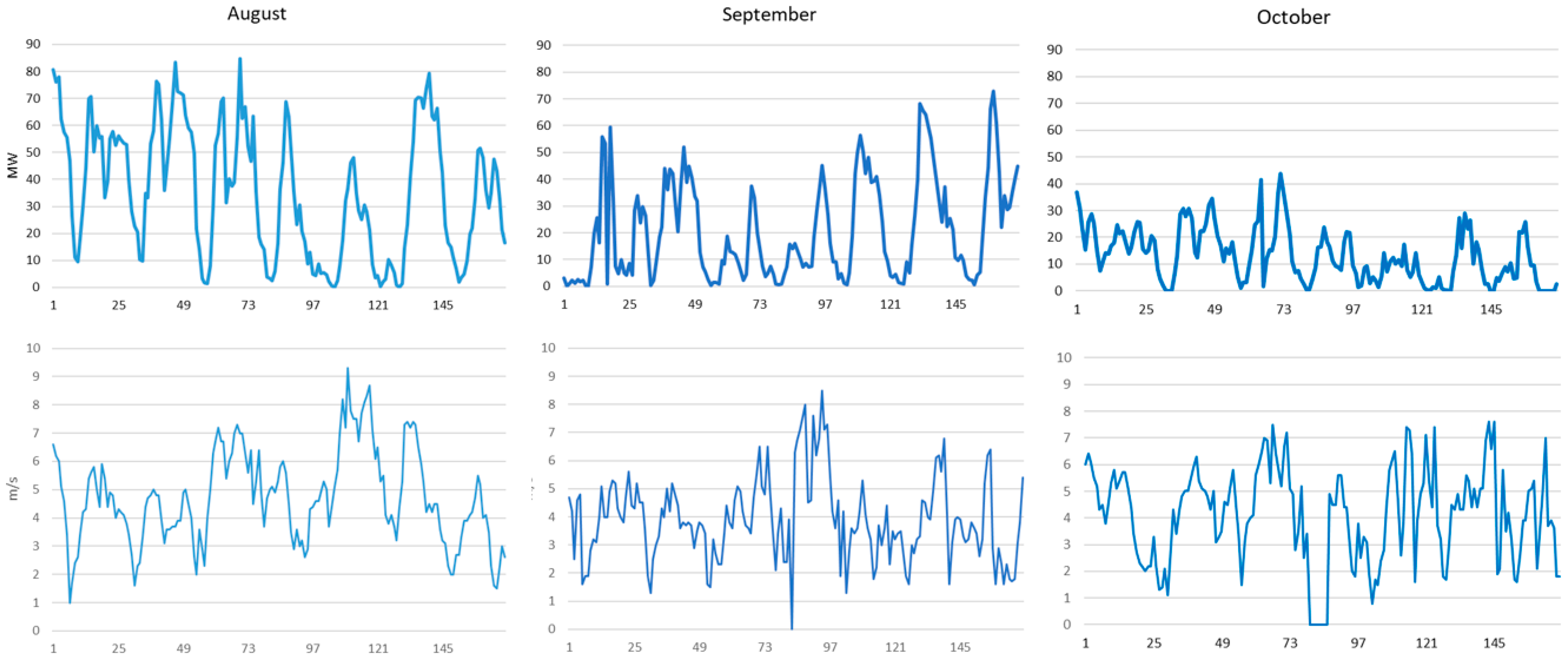
As regards the wind farms, a more complex dependency exists between wind power and air density, which is strictly correlated with temperature and humidity [31]. Hence, wind power depends mostly on wind speed. Figure 11 illustrates the seasonal power generation using PVs against the cloud coverage, while the stochastic contribution of wind is presented in Figure 12.

4.2. Results and Discussion

To discuss the results and how they could be interpreted from the perspective of future studies, 3 case studies and 13 training algorithms are taken into account. The difference between them lies in the different number of predictors used in each case. The aim is to identify whether an algorithm functions better with fewer input predictors (due to a probable difficulty in acquiring historical data) and which one occurs advantageous in terms of best performance. The forecasting accuracy of the imposed algorithms is calculated in terms of the mean absolute error (MAE), the root mean square error (RMSE), the mean absolute percentage error (MAPE), the mean absolute range normalized error (MARNE), and the determination coefficient R-squared (R²) between the actual (P_a) and predicted (P_p) residual load. Denoting with $\overline{P_a}$ the average residual load for τ time steps, the error metrics are calculated via Equations (26)–(30).

$$MAE={\displaystyle \frac{1}{\tau }}\sum _{t=1}^{\tau }\left|P_a\left(t\right)-P_p\left(t\right)\right|$$

(26)

$$RMSE={\displaystyle \frac{1}{\tau }}\sqrt{\sum _{t=1}^{\tau }{\left(P_a\left(t\right)-P_p\left(t\right)\right)}^2}$$

(27)

$$MAPE={\displaystyle \frac{1}{\tau }}\sum _{t=1}^{\tau }\left|{\displaystyle \frac{P_a\left(t\right)-P_p\left(t\right)}{P_a\left(t\right)}}\right|$$

(28)

$$MARNE={\displaystyle \frac{1}{\tau }}\sum _{t=1}^{\tau }{\displaystyle \frac{\left|P_a\left(t\right)-P_p\left(t\right)\right|}{\underset{t}{\max }{P}_a\left(t\right)}}\times 100$$

(29)

$$R^2=1-{\displaystyle \frac{\sum _{t=1}^{\tau }{\left(P_a\left(t\right)-P_p\left(t\right)\right)}^2}{\sum _{t=1}^{\tau }{\left(P_a\left(t\right)-\overline{P_a}\right)}^2}}$$

(30)

Regarding the parameter settings, for simulation purposes the learning rate was set to 0.01 as the initial momentum update. The decrease and increase factor remained at 0.1 and 2.5, respectively, while the maximum momentum was set at 20.10¹⁰. The number of neurons varies for each implementation based on the configuration [n₁ (n₁ + 2) (n₁ + 3) (n₁ + 2) n₁], where n₁ accounts for the number of input predictors at each case. Finally, the performance goal was set to 10⁻⁶ with a maximum number of epochs training 1000 and 200 validation failures. The first case study makes use of minimum inputs considering the hour of the day t; the day of the year d; and the temperature for the load target, the hour of the day for the PV generation, and the wind speed solely for the target of wind power production. The inputs in this case are formulated as follows:

$$X_1=\left\{\begin{array}{c}t,d\\ t\\ v_w\end{array}\right.$$

(31)

The respective results obtained by the employed algorithms are listed in

Table 4. Performance indices pertaining case study 1.

Algorithm	MAE	RMSE	MAPE	MARNE	R2
trainlm	52.0579	0.70639	0.11098	5.51395	0.763704
trainbfg	65.4909	0.8779	0.1403	6.9368	0.635
trainrp	64.4048	0.8660	0.1356	6.8217	0.6449
trainscg	67.0164	0.8934	0.1417	7.0984	0.6220
traincgb	56.2291	0.7758	0.1206	5.9558	0.7295
traincgf	96.4177	1	0.2083	10.2125	0.2499
traincgp	57.8913	0.7751	0.1253	6.1318	0.7155
trainoss	57.3835	0.7708	0.1245	6.078	0.7186
trainbr	51.2384	0.7052	0.1098	5.4272	0.7645
traingd	379.0277	4.9587	0.8204	40.1465	−10.6439
traingdm	198.1535	2.5655	0.4310	20.9884	−2.1168
traingda	87.2362	1.1631	0.1960	9.2400	0.3594

.

Based on the obtained results, the Bayesian regularization algorithm outperforms the alternatives in terms of MAE, RMSE, MAPE, MARNE, and R² performance indices. Following is the Levenberg–Marquardt backpropagation algorithm, which offers quite high accuracy with minor deviations from the first. The gradient descent approach fails in fitting the target with high accuracy, providing a slight improvement with momentum backpropagation and adaptive learning. During the second case, the assessed algorithms utilize a normal number of inputs widely achievable. Thus, for the load target, the month of the year (m), the season of the year (s), the year (y), the temperature, the humidity, and the day type (D) have been also considered as predictor inputs. The RES targets accounted for the day, month, season, year, and cloud coverage for PV output, and temperature for the respective wind output. In this way, the predictor in the underlying study transformed into the following:

$$X_2=\left\{\begin{array}{c}t,d,m,s,y,T,H,D\\ t,d,m,s,y,C\\ v_w,T\end{array}\right.$$

(32)

Apart from the traincgb, trainoss, and all gradient-descent based algorithms, the rest of the alternatives showed improved performance. Although the Levenberg–Marquardt algorithm provided a minor improvement, Bayesian regularization training demonstrated a proven accuracy, increasing the performance difference by its competitors. The respective results are tabulated in

Table 5. Performance indices pertaining to case study 2.

Algorithm	MAE	RMSE	MAPE	MARNE	R2
trainlm	52.7104	0.7166	0.1135	5.5831	0.7568
trainbfg	59.5057	0.7976	0.1280	6.3028	0.6988
trainrp	51.3698	0.6995	0.1115	5.4413	0.7683
trainscg	53.6320	0.731115629	0.1157	5.6807	0.7469
traincgb	56.6209	0.7618	0.1221	5.9973	0.7251
traincgf	66.2414	0.8969	0.1422	7.0163	0.6191
traincgp	56.7489	0.7782	0.1209	6.0108	0.7132
trainoss	58.2981	0.7871	0.1245	6.1749	0.7066
trainbr	46.2131	0.6349	0.099	4.8949	0.8091
traingd	573.3197	6.7253	1.3112	60.7259	−20.4185
traingdm	357.1059	4.2111	0.8105	37.8246	−7.3976
traingda	93.1269	1.2261	0.1963	9.8640	0.2882

.

Finally, the accuracy of the proposed MIMO model is examined by assessing the respective algorithms using an enhanced number of input predictors. These consolidate the current fuel price and past knowledge in load target considering also the electricity, the previous day load ($P_{load}^{\prime }$), the previous week load ($P_{load}^{″}$), and the previous year load ($P_{load}^{‴}$). Accordingly, the weather variables of temperature and humidity are simultaneously included as predictors for both PV and wind power targets. This converts (32) as follows:

$$X_3=\left\{\begin{array}{c}t,d,m,s,y,T,H,D,c_f,c_{el}^{\prime },P_{load}^{\prime },P_{load}^{″},P_{load}^{‴}\\ t,d,m,s,y,C,T,H\\ v_w,T,H\end{array}\right.$$

(33)

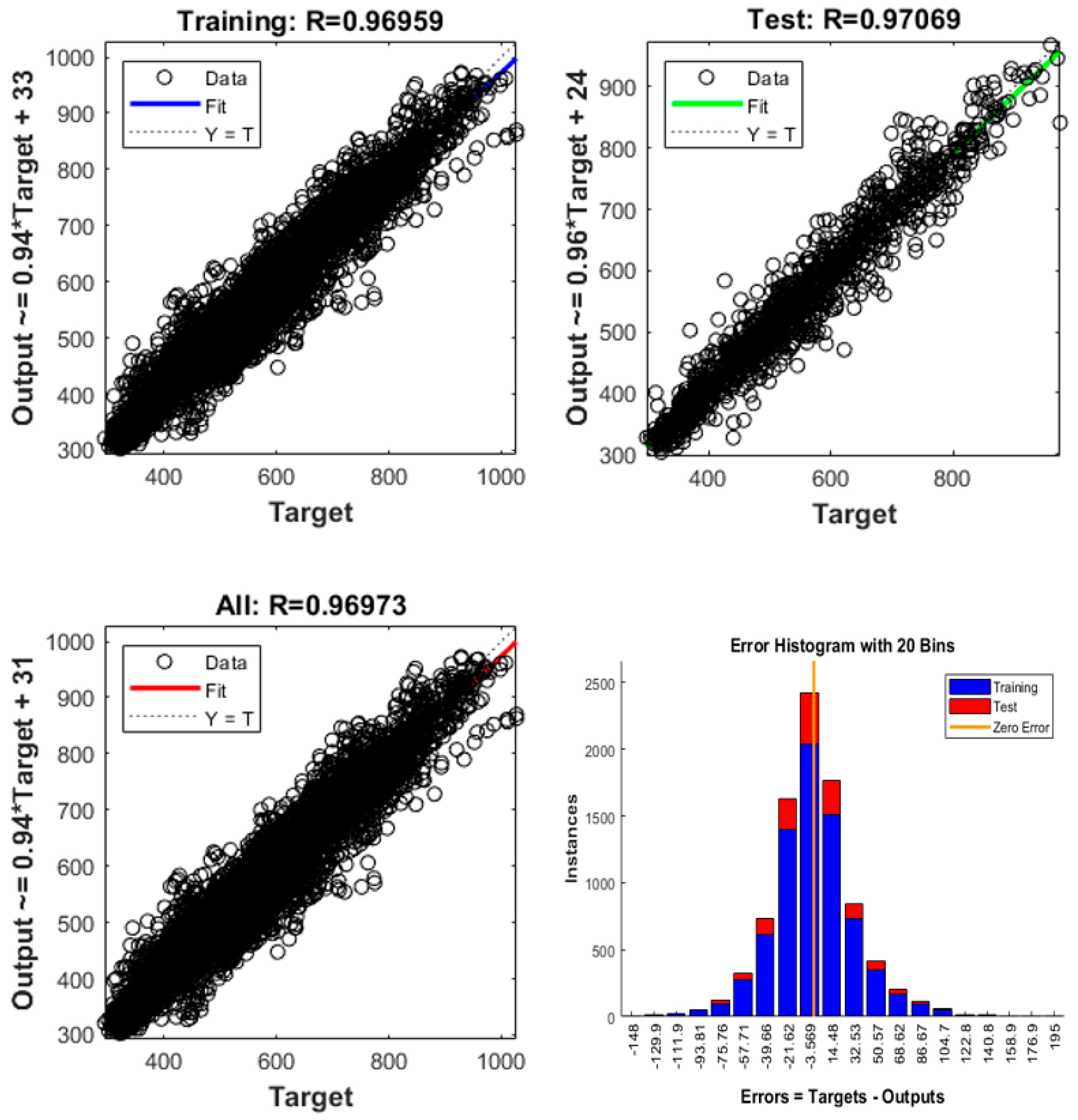
As expected, the Levenberg–Marquardt and Bayesian regularization training algorithms achieve superior performance against the others in terms of MAE, MAPE, MARNE, and R² indices, slightly favouring Bayesian regularization (trainbr). The Fletcher–Power conjugate gradient (traincgf) appears advantageous when comparing the RMSE performance. Figure 13 depicts the regression diagrams for the trainbr algorithm and enhanced predictor inputs. Testing and validation ranges show a narrower band compared to the training range. This stems from the fact that the selected training rate was 70% in contrast to the 15% of the test and validation cases, a combination selected after comparing three training–testing–validation alternatives, namely 50-25-25, 60-20-20, and 70-15-15.

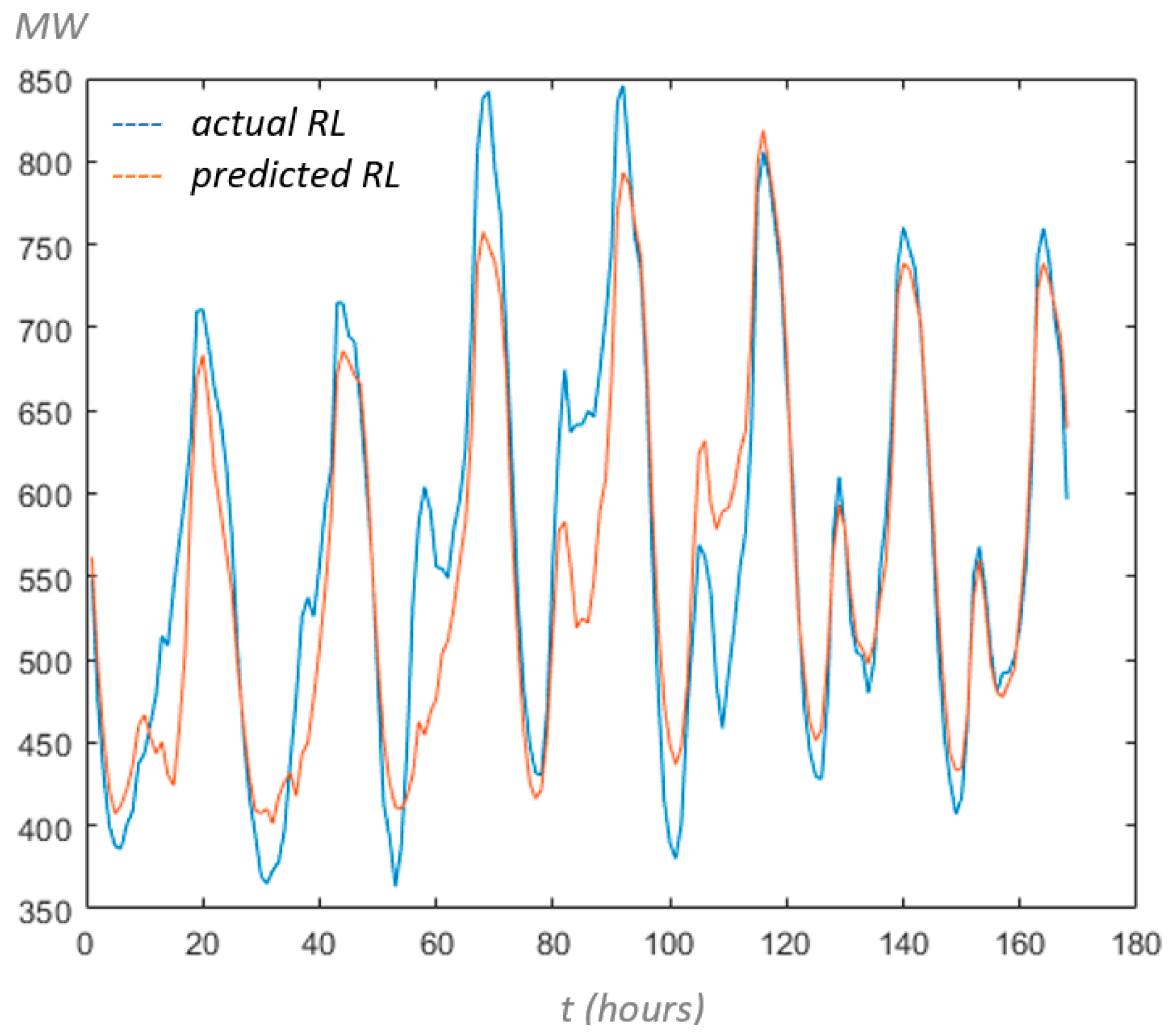
It is worth noting that in the third case where enhanced inputs were taken into account for training purposes, all algorithms showed considerable improvements against the first and second case studies. The obtained results relating to the algorithms assessed in the third case study are shown in

Table 6. Performance indices pertaining case study 3.

Algorithm	MAE	RMSE	MAPE	MARNE	R2
trainlm	31.8937	0.4545	0.0687	3.3782	0.9022
trainbfg	36.9099	0.5238	0.079	3.9095	0.8701
trainrp	38.5916	0.5429	0.0833	4.0876	0.8604
trainscg	37.9135	0.5412	0.0809	4.0158	0.8613
traincgb	35.2977	0.501	0.0758	3.7387	0.8812
traincgf	35.098	0.4493	0.0752	3.7176	0.882
traincgp	35.1019	0.4983	0.0755	3.718	0.8824
trainoss	37.3	0.5275	0.0799	3.9508	0.8682
trainbr	31.6578	0.4556	0.0681	3.3532	0.9017
traingd	244.8243	3.1092	0.5686	25.9317	−3.5779
traingdm	84.4704	1.1370	0.1809	8.9471	0.3878
traingda	49.9334	0.6833	0.1078	5.2889	0.7789

. To display the contrast with trainbr, the forecasted residual load demand for a representative week in the worst case (in winter) is presented in Figure 14 against the actual residual load. In order to provide a direct comparison between the best candidate and potential competitors, the respective best output can be observed in Figure 15. The quantification of uncertainty due to the variability in renewable energy was estimated in terms of MAE, RMSE, and MARNE. PV generation presented an annual variation of ±0.72, ±0.2, and ±0.35, respectively. The corresponding errors for the generated wind are evaluated at ±1.6, ±0.04, and ±3.7.

Repeating the experiments with varying hidden layers, the obtained results were similar, leading to identical performance indices. Consequently, there is no need of high-level abstraction because of the noncomplex relation between inputs and outputs. In this way, the same results can be achieved with traditional neural networks conserving vast computational efforts.

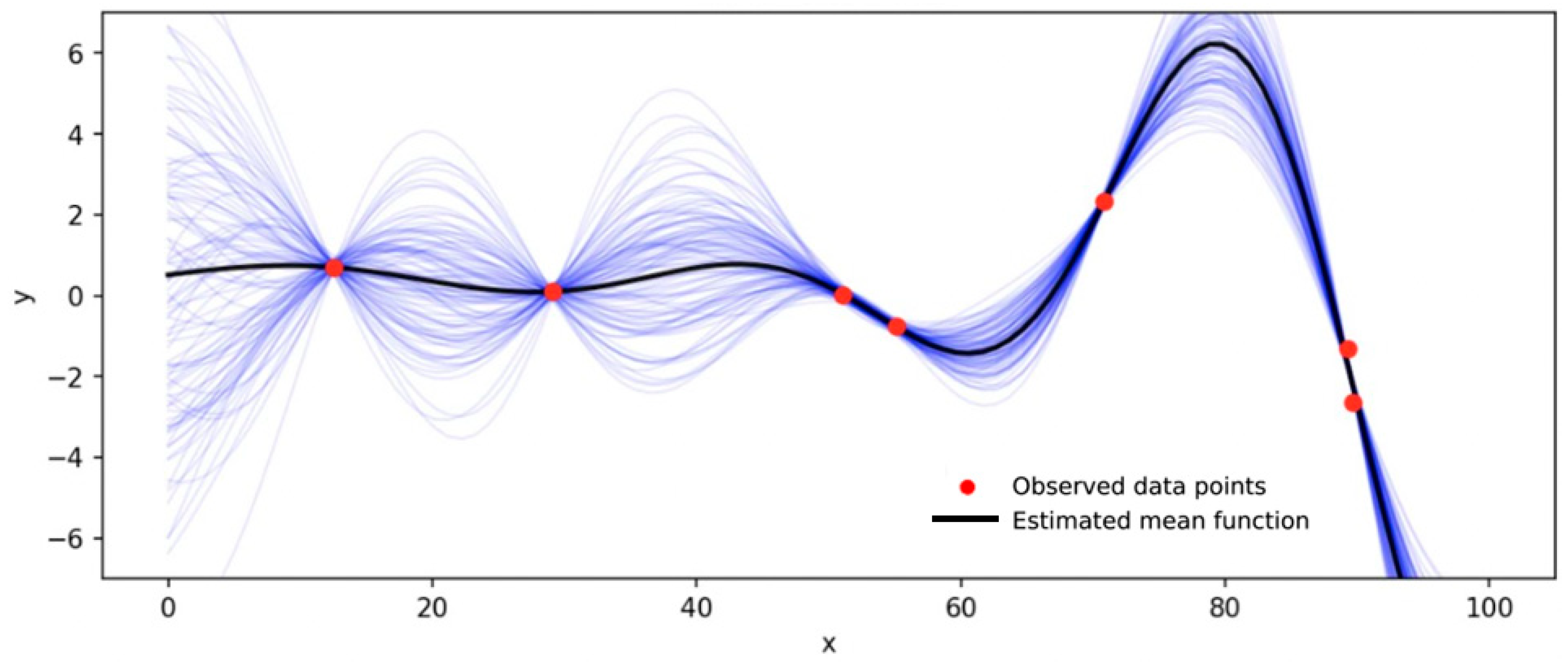
Applying GPR, the obtained results appear promising, offering increased performance. The accuracy has been drastically improved in the expense of computational effort. In contrast to parametric formulations which give only point estimations, GPR provides a probabilistic framework with uncertainty estimates for prediction. In this way, it is able to capture complex relationships in data, enhancing flexibility. Figure 16 demonstrates a typical example of the estimated mean function over the observed data points.

Since computational speed is crucial for day-ahead forecasting, the performance, in terms of time, of each algorithm must be taken into account. Defining the times each algorithm visits the dataset to update weights as epochs, the following

Table 7. Epochs and average execution times (AET-bold values) pertaining the examined algorithms.

	trainlm	trainbfg	trainrp	trainscg	traincgb	traincgf	traincgp	trainoss	trainbr	traingd	traingdm	traingda	traingdx
Case 1	22	188	62	47	64	26	75	16	54	6	6	38	30
Case 2	34	863	82	24	14	59	19	49	163	6	6	39	121
Case 3	18	1000	50	31	32	71	36	13	162	6	72	35	36
AET (s)	14	102	5	4	13	5	4	11	87	0	0	0	1

lists this feature for the examined case studies.

Although GPR can be adequately applied for time-series forecasting, it appears very computationally expensive when dealing with large datasets. This can be mainly derived from the required inversion of the covariance matrix. As a result, the increasing number of predictors complicates the fitting task and adds considerable efforts that can become extremely time-intensive. Since the day-ahead prognosis requires low execution times that do not exceed a few minutes, the simulation experiments were limited to the forecast of wind power generation which imposes the fewest input predictors. The remaining inputs can be predicted by making use of neural-based models, and the underline target of residual load can be evaluated with the aid of a parallel configuration of the MIMO depicted in Figure 17.

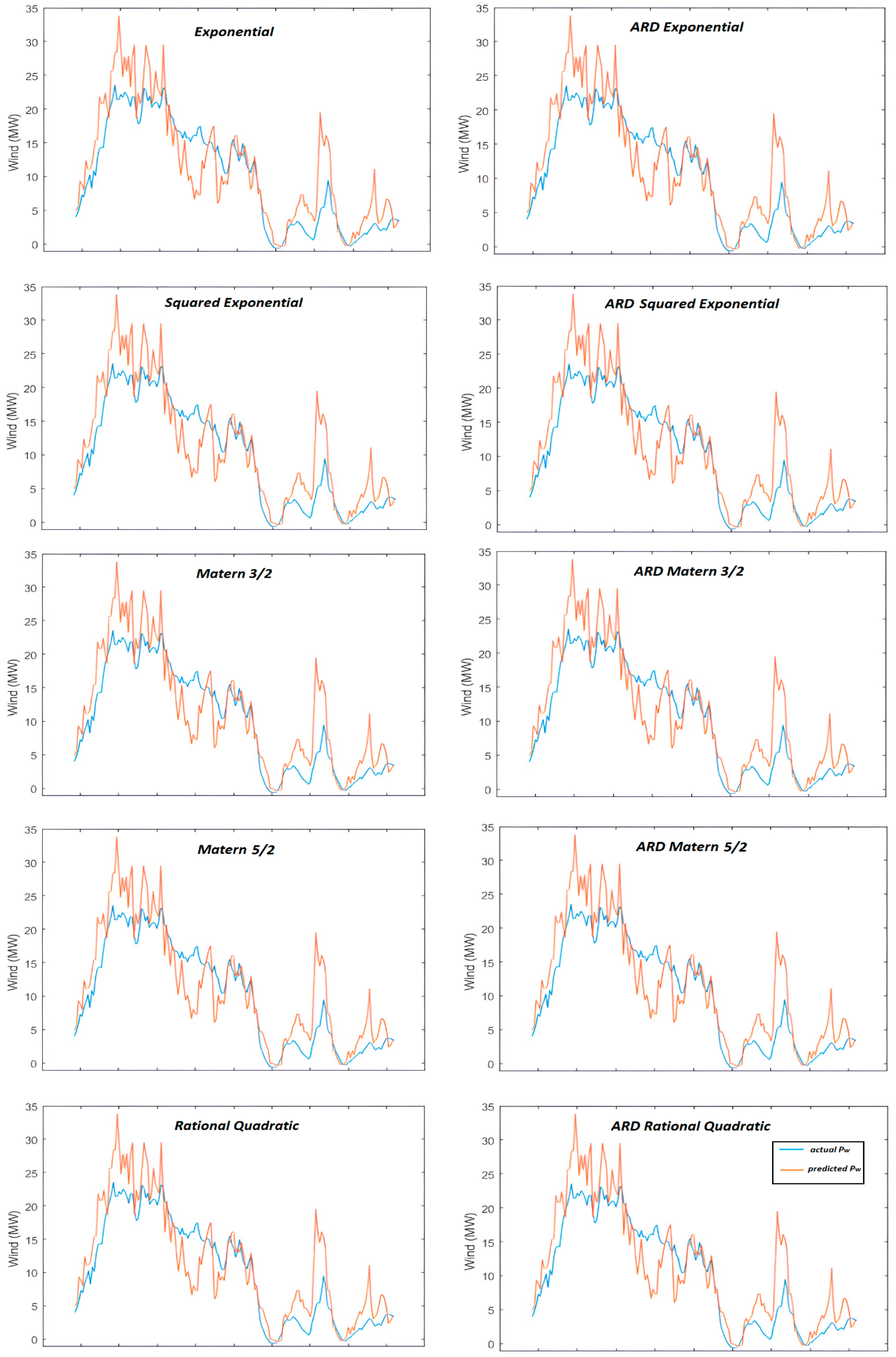
In order to gain a broad overview of the performance between kernels with the same and a separate length scale for each predictor, Figure 18 illustrates the wind power prediction over the actual generation. The depicted outcome refers to a specific day in 2021 which was characterized by extreme weather conditions and strongly fluctuating wind speeds with continuous changes in its direction. At first glance, it can be concluded that all kernels give similar predictions that contain several inaccuracies. The contrasts arise from the calculation of the performance indices, where the ARD exponential appears superior followed by ARD Matern 3/2. Their overall achievements are summarised in

Table 8. Kernel performance indices pertaining the parallel ANN-GPR in case study 3.

Algorithm	MAE	RMSE	MAPE	MARNE	R2
Exponential	3.0133	0.0180	1.1259	3.6771	0.9395
ARD exponential	2.8838	0.0175	1.1029	3.5191	0.9429
Squared exponential	4.5092	0.0249	4.1842	5.5026	0.8846
ARD squared exponential	3.2132	0.0195	1.1350	3.9211	0.9292
Matern 3/2	3.9574	0.0219	3.5578	4.8292	0.9105
ARD Matern 3/2	3.0244	0.0184	1.1317	3.6907	0.9370
Matern 5/2	4.3099	0.0237	4.2216	5.2594	0.8955
ARD Matern 5/2	3.0976	0.0189	1.1422	3.7800	0.9339
Rational quadratic	4.4132	0.0244	4.1132	5.3854	0.8896
ARD rational quadratic	3.1616	0.0192	1.1540	3.8582	0.9313

. The obtained results regard case study 3, where wind speed, relative humidity, and temperature constitute the only predictor inputs for prognosis.

5. Conclusions

The required operating reserves to balance the mismatches between actual and forecasted power add considerable costs to the total electricity generation in the presence of renewable sources. Efficient and adequate tools are needed in order to enhance the forecasting accuracy of residual-load prognosis in the upcoming smart grids. In this study, a multi-input/multi-output model is proposed to improve system security and reliability. Specifically, based on a feed-forward deep neural network employed to map the relationship between multiple inputs and output targets, the model is assessed by utilizing 13 different training algorithms. The assessment was performed with simulations based on annual, actual data relating to the islanded system of Cyprus under three case studies. This constitutes a benchmark framework for the testing and validation of future novel forecast models by making use of minimum, normal, and enhanced predictors and multiple highly variable targets. Apart from the historical data size, the added predictive information facilitates decreasing the error between the actual and predicted targets. For example, the forecasted demand based on the weather impact (such as temperature and humidity) appears inadequate to observe the share due to the increasing load from one year to another. This characteristic is retrieved by making use the previous load information, which provides the trend of increasing load because of either new electrical installations or prolonged tourism accommodation. The same occurs in renewable contribution where more predictors correlated with weather conditions allow for better output prognosis.

Varying the number of input predictors, the Levenberg–Marquardt and Bayesian regularization algorithms outperform their competitors in forecasting in terms of the mean absolute error, the root mean square error, the mean absolute percentage error, the mean absolute range normalized error, and the determination coefficient. With enhanced input predictors during the third case study, the Bayesian regularization mechanism achieved a superior mean absolute error < 31 MW and 0.9017 determination coefficient. Showing vigorous improvement between the underlying studies, this puts it in the first place of choice for load forecasts in the presence of strongly variable wind and PV contributions. Increasing the hidden layers to compare the outcome in deep learning, the obtained results showed similar behaviour without improving the overall performance indices. On the contrary, the execution times increased, disadvantaging their application in day-ahead forecasting tasks. This achievement reveals the importance of using optimization towards minimizing the fitting error during the training process. Therefore, for future directions to research, it is indicated to involve Gaussian process-based Bayesian optimization to further improve the performance indices in systems with increased stochastic inputs such that of renewable energy sources. A wide variety of kernel functions can be used, combining proper Bayesian inference strategies to minimize the fitness loss and optimally define the involved hyperparameters. In each case, the best-fit kernel choice can be engaged with a different target, leading to improved performance metrics with respect to residual load forecasts. Apart from the training–testing–validation optimum combination, a further aspect can also take into account the optimal neural size (or network configuration) in parallel configurations of multi-input/multi-output artificial models.

References

1. Nikolaidis, P.; Poullikkas, A. A Thorough Emission-Cost Analysis of the Gradual Replacement of Carbon-Rich Fuels with Carbon-Free Energy Carriers in Modern Power Plants: The Case of Cyprus. Sustainability 2022, 14, 10800. [Google Scholar] [CrossRef]
2. Khosravi, A.; Koury, R.; Machado, L.; Pabon, J. Prediction of wind speed and wind direction using artificial neural network, support vector regression and adaptive neuro-fuzzy inference system. Sustain. Energy Technol. Assess. 2018, 25, 146–160. [Google Scholar] [CrossRef]
3. Khosravi, A.; Koury, R.; Machado, L.; Pabon, J. Prediction of hourly solar radiation in Abu Musa Island using machine learning algorithms. J. Clean. Prod. 2018, 176, 63–75. [Google Scholar] [CrossRef]
4. Pierro, M.; De Felice, M.; Maggioni, E.; Moser, D.; Perotto, A.; Spada, F.; Cornaro, C. Residual load probabilistic forecast for reserve assessment: A real case study. Renew. Energy 2019, 149, 508–522. [Google Scholar] [CrossRef]
5. Shi, H.; Xu, M.; Li, R. Deep Learning for Household Load Forecasting—A Novel Pooling Deep RNN. IEEE Trans. Smart Grid 2018, 9, 5271–5280. [Google Scholar] [CrossRef]
6. Kong, W.; Dong, Z.Y.; Jia, Y.; Hill, D.J.; Xu, Y.; Zhang, Y. Short-Term Residential Load Forecasting Based on LSTM Recurrent Neural Network. IEEE Trans. Smart Grid 2017, 10, 841–851. [Google Scholar] [CrossRef]
7. Kong, W.; Dong, Z.Y.; Hill, D.J.; Luo, F.; Xu, Y. Short-Term Residential Load Forecasting Based on Resident Behaviour Learning. IEEE Trans. Power Syst. 2017, 33, 1087–1088. [Google Scholar] [CrossRef]
8. Chang, G.; Lu, H.; Chang, Y.; Lee, Y. An improved neural network-based approach for short-term wind speed and power forecast. Renew. Energy 2017, 105, 301–311. [Google Scholar] [CrossRef]
9. Kumar, G.; Malik, H. Generalized Regression Neural Network Based Wind Speed Prediction Model for Western Region of India. Procedia Comput. Sci. 2016, 93, 26–32. [Google Scholar] [CrossRef]
10. Mi, X.-W.; Liu, H.; Li, Y.-F. Wind speed forecasting method using wavelet, extreme learning machine and outlier correction algorithm. Energy Convers. Manag. 2017, 151, 709–722. [Google Scholar] [CrossRef]
11. Kaplan, O.; Temiz, M. A novel method based on Weibull distribution for short-term wind speed prediction. Int. J. Hydrogen Energy 2017, 42, 17793–17800. [Google Scholar] [CrossRef]
12. Yu, C.; Li, Y.; Bao, Y.; Tang, H.; Zhai, G. A novel framework for wind speed prediction based on recurrent neural networks and support vector machine. Energy Convers. Manag. 2018, 178, 137–145. [Google Scholar] [CrossRef]
13. Salisu, S.; Mustafa, M.W.; Mustapha, M. A Wavelet Based Solar Radiation Prediction in Nigeria Using Adaptive Neuro-Fuzzy Approach. Indones. J. Electr. Eng. Comput. Sci. 2018, 12, 907–915. [Google Scholar] [CrossRef]
14. Khosravi, A.; Nunes, R.; Assad, M.; Machado, L. Comparison of artificial intelligence methods in estimation of daily global solar radiation. J. Clean. Prod. 2018, 194, 342–358. [Google Scholar] [CrossRef]
15. Kothona, D.; Panapakidis, I.P.; Christoforidis, G.C. A novel hybrid ensemble LSTM-FFNN forecasting model for very short-term and short-term PV generation forecasting. IET Renew. Power Gener. 2021, 16, 3–18. [Google Scholar] [CrossRef]
16. Dudek, G. Pattern-based local linear regression models for short-term load forecasting. Electr. Power Syst. Res. 2016, 130, 139–147. [Google Scholar] [CrossRef]
17. Tian, C.; Ma, J.; Zhang, C.; Zhan, P. A Deep Neural Network Model for Short-Term Load Forecast Based on Long Short-Term Memory Network and Convolutional Neural Network. Energies 2018, 11, 3493. [Google Scholar] [CrossRef]
18. Xu, S.; Guo, S. Distributed Reactive Power Optimization for Energy Internet via Multiagent Deep Reinforcement Learning with Graph Attention Networks. IEEE Trans. Ind. Inform. 2024, 20, 8696–8706. [Google Scholar] [CrossRef]
19. Zhang, N.; Yan, J.; Hu, C.; Sun, Q.; Yang, L.; Gao, D.W.; Guerrero, J.M.; Li, Y. Price-Matching-Based Regional Energy Market with Hierarchical Reinforcement Learning Algorithm. IEEE Trans. Ind. Inform. 2024, 20, 11103–11114. [Google Scholar] [CrossRef]
20. Yang, Y.; Wu, J.; Chen, Y.; Li, C. A New Strategy for Short-Term Load Forecasting. Abstr. Appl. Anal. 2013, 2013, 208964. [Google Scholar] [CrossRef]
21. Yang, D.; Guo, J.-E.; Li, J.; Wang, S.; Sun, S. Knowledge Mapping in Electricity Demand Forecasting: A Scientometric Insight. Front. Energy Res. 2021, 9, 771433. [Google Scholar] [CrossRef]
22. Nikolaidis, P. Variational Bayes to Accelerate the Lagrange Multipliers towards the Dual Optimization of Reliability and Cost in Renewable Energy Systems. Algorithms 2022, 16, 20. [Google Scholar] [CrossRef]
23. Dubey, S.; Sarvaiya, J.N.; Seshadri, B. Temperature Dependent Photovoltaic (PV) Efficiency and Its Effect on PV Production in the World—A Review. Energy Procedia 2013, 33, 311–321. [Google Scholar] [CrossRef]
24. Bergin, M.H.; Ghoroi, C.; Dixit, D.; Schauer, J.J.; Shindell, D.T. Large Reductions in Solar Energy Production Due to Dust and Particulate Air Pollution. Environ. Sci. Technol. Lett. 2017, 4, 339–344. [Google Scholar] [CrossRef]
25. Konstantinou, M.; Peratikou, S.; Charalambides, A.G. Solar Photovoltaic Forecasting of Power Output Using LSTM Networks. Atmosphere 2021, 12, 124. [Google Scholar] [CrossRef]
26. Peratikou, S.; Charalambides, A.G. Estimating clear-sky PV electricity production without exogenous data. Sol. Energy Adv. 2022, 2, 100015. [Google Scholar] [CrossRef]
27. Bilski, J.; Smoląg, J.; Kowalczyk, B.; Grzanek, K.; Izonin, I. Fast Computational Approach to the Levenberg-Marquardt Algorithm for Training Feedforward Neural Networks. J. Artif. Intell. Soft Comput. Res. 2023, 13, 45–61. [Google Scholar] [CrossRef]
28. CERA. CERA 2020 Annual Report. 2020. Available online: https://www.cera.org.cy/Templates/00001/data/ektheseis/2022_en.pdf (accessed on 27 August 2024).
29. Livera, A.; Paphitis, G.; Theristis, M.; Lopez-Lorente, J.; Makrides, G.; Georghiou, G.E. Photovoltaic System Health-State Architecture for Data-Driven Failure Detection. Solar 2022, 2, 81–98. [Google Scholar] [CrossRef]
30. Kraskov, A.; Stögbauer, H.; Grassberger, P. Estimating mutual information. Phys. Rev. E Stat. Phys. Plasmas Fluids Relat. Interdiscip. Top. 2004, 69, 066138. [Google Scholar] [CrossRef]
31. Nikolaidis, P. Wind power forecasting in distribution networks using non-parametric models and regression trees. Discov. Energy 2022, 2, 6. [Google Scholar] [CrossRef]
Figure 1. Daily configurations of summer demand in the presence of RES.
Energies 17 05219 g001
Figure 2. “Duck curve” variation in the presence of storage and incentivised prosumer participation.
Energies 17 05219 g002
Figure 3. Simulation of wind direction diagram for an upwind turbine.
Energies 17 05219 g003
Figure 4. Paradigm of a PV generation system with two-axis tracking system.
Energies 17 05219 g004
Figure 5. Demonstration of the proposed neural-based multi-input/multi-output (MIMO) model.
Energies 17 05219 g005
Figure 6. Distribution of the annual MW-power for load, PV, and wind.
Energies 17 05219 g006
Figure 7. Actual and statistical annual loading (MW) for demand and RES generation.
Energies 17 05219 g007
Figure 8. Monthly temperature extremities (°C) and average humidity (%).
Energies 17 05219 g008
Figure 9. Stepped histograms for the (a) cloudiness and (b) respective average temperatures.
Energies 17 05219 g009
Figure 10. Load demand relation with temperature and humidity during (a) winter and (b) summer.
Energies 17 05219 g010
Figure 11. PV contribution for a representative week per season.
Energies 17 05219 g011
Figure 12. Hourly variation in wind power and wind speed for three random weeks.
Energies 17 05219 g012
Figure 13. Bayesian regularization regression and error histogram diagrams for the case study 3.
Energies 17 05219 g013
Figure 14. Actual vs. forecasted residual load (RL) based on Bayesian regularization algorithm.
Energies 17 05219 g014
Figure 15. Actual vs. forecasted residual load (RL) of training algorithm alternatives (blue line –actual, red line-predicted).
Energies 17 05219 g015
Figure 16. Typical implementation of Gaussian process regression.
Energies 17 05219 g016
Figure 17. Demonstration of the parallel ANN-GPR MIMO model.
Energies 17 05219 g017
Figure 18. Actual vs. forecasted wind production derived by using different kernel types.
Energies 17 05219 g018