Machine Learning-Based Predictions of Flow and Heat Transfer Characteristics in a Lid-Driven Cavity with a Rotating Cylinder

Abstract

Machine learning-based predictions of heat transfer characteristics in lid-driven cavities are transforming the field of computational fluid dynamics (CFD). Lid-driven cavities are a fundamental problem in fluid mechanics, characterized by the motion of a fluid inside a square cavity driven by the motion of one of its walls. The goal of this study was to develop multiple machine-learning regression models and highlight the discrepancies between the predicted and actual average Nusselt numbers. Additionally, the study utilized physics-informed neural networks (PINNs) to model the flow and thermal behavior at both low and high Reynolds numbers. The results were compared among actual data from computational fluid dynamics (CFD) simulations, PINN models trained with CFD data, and purely PINN models created without any prior data input. The findings of this study showed that the random forest model exhibited an exceptional stability in its predictions, consistently maintaining low errors even as the Reynolds number increased compared with other machine-learning regression models. Further, the results of this study in terms of flow and thermal behavior within the cavity were found to depend significantly on the PINN method. The data-driven PINN exhibited a much lower mean average errors at both Reynolds numbers, while the physics-based PINN showed lower physics loss.

1. Introduction

The lid-driven cavity flow problem is a fundamental scenario encountered in various engineering applications, including solar systems, microelectronics, and nuclear reactors [1,2,3,4,5]. It generally involves a square cavity with a top lid that moves at a constant velocity, generating complex flow patterns within the cavity. Introducing a rotating cylinder at the center of the cavity adds a layer of complexity, as it generates additional vortices and influences the flow structure [6,7]. For instance, Ghaddar [8] examined mixed convection heat transfer resulting from the interaction between natural convection and a rotating cylindrical heat source in a rectangular enclosure. The findings of that study indicated that the heat transfer rate due to the cylinder’s rotation was affected by the cylinder’s position within the enclosure. Liao and Lin [9] explored mixed convection flow and heat transfer in a cavity containing a heated rotating cylinder, examining various parameters such as the Rayleigh number, Prandtl number, and aspect ratio. Their findings revealed that smaller aspect ratios resulted in higher Nusselt numbers, while the cylinder’s rotation led to a reduction in the average Nusselt number. Khanafer and Aithal [6] conducted a numerical analysis of mixed convection heat transfer in a lid-driven cavity with a rotating cylinder, focusing on two key parameters: the Richardson number, the non-dimensional angular velocity of the cylinder, and the direction of rotation. The simulation results were validated using the open-source spectral element code, Nek5000, and were presented through streamlines, isotherms, and average and local Nusselt numbers. Their findings demonstrated that the average Nusselt number was affected by the direction of the cylinder’s angular velocity. Specifically, the average Nusselt number increased with an increase in the clockwise angular velocity of the cylinder across various Richardson numbers. Khanafer et al. [7] numerically studied mixed convection heat transfer in a differentially heated cavity with two rotating cylinders, considering parameters like Richardson number, Reynolds number, cylinder rotation speed, and location. The results, validated using the Nek5000 code, showed that the average Nusselt number was significantly affected by the cylinder’s rotation speed, Reynolds number, and Richardson number, though it becomes independent of rotation speed at a high Richardson number (Ri = 10). The direction of rotation was also found to play a crucial role, changing both the average Nusselt number and flow patterns.

Solving this problem using traditional computational fluid dynamics (CFD) methods requires solving the Navier–Stokes equations, which can be computationally intensive, especially when multiple simulations are needed for different parameters like cylinder rotation speed, Reynolds number, or lid velocity, and Richardson number. Recently, machine learning (ML) is transforming various fields by enabling more efficient data analysis, predictive modeling, and optimization. In areas like healthcare, robotics, and autonomous systems, ML algorithms have revolutionized decision-making processes by offering accurate predictions and uncovering patterns in complex datasets [10,11]. In the field of fluid mechanics and heat transfer, ML has shown significant promise by reducing the computational cost and time associated with solving complex problems. For example, ML models can be trained on high-fidelity simulation data to predict flow patterns, temperature distributions, and turbulence characteristics without the need for extensive numerical simulations [12,13,14,15]. This capability allows for real-time analysis and design optimization, which is particularly valuable in applications such as aerospace, automotive design, and energy systems.

Additionally, ML techniques like neural networks and Gaussian process regression (GPR) are being used to enhance the accuracy of simulations and to develop new insights into the underlying physics of fluid flow and heat transfer processes [16,17,18,19]. Selimefendigil and Öztop [20] numerically investigated mixed convection in a nanofluid-filled square cavity with ventilation ports and an adiabatic rotating cylinder, using COMSOL to solve the governing equations. The effects of the Grashof number, Reynolds number, nanoparticle volume fraction, and cylinder rotation angle on the flow and thermal fields are analyzed. The generalized regression neural network (GRNN) was used to predict thermal performance, showing that heat transfer increased linearly with higher nanoparticle volume fractions and clockwise rotation. The GRNN outperformed radial basis and feed-forward networks in predicting thermal outcomes. Tizakast et al. [21] explored the use of machine-learning models to analyze double-diffusive natural convection in rectangular cavities filled with non-Newtonian fluids. The flow was characterized by four dimensionless parameters: thermal Rayleigh number, Lewis number, buoyancy ratio, and power-law behavior index, which were used as input features. Another study explored the use of surrogate models to optimize surface textures for enhanced heat transfer in cavity flows [22], by coupling genetic algorithms with ML-based surrogates, and it was found that a significant reduction in optimization time was possible while maintaining high predictive accuracy. This approach demonstrates the potential of ML to revolutionize design processes in engineering applications, particularly in scenarios demanding high precision and computational efficiency. To accurately model fluid flow, the study predicted three key characteristics: flow intensity, the average Nusselt number, and the average Sherwood number, utilizing four machine-learning models: artificial neural networks (ANN), random forests (RF), gradient boosted decision trees (GBDT), and extreme gradient boosting (XGBoost v2.1.1). This paper confirmed the effectiveness of using a machine-learning approach to model non-Newtonian double-diffusive fluid flows.

As ML continues to evolve, its integration with traditional methods is likely to lead to breakthroughs in both efficiency and understanding across these critical fields. It is evident from the cited literature that the use of machine learning to predict flow and heat transfer in a lid-driven cavity with a rotating cylinder at its center has not been explored. Most of the investigations were focused on flow and heat transfer in a lid-driven cavity [23,24,25,26]. Accurately capturing the multi-physics interactions—such as the coupling between fluid flow, heat transfer, and rotational dynamics—demands advanced machine-learning architectures capable of learning these complex dependencies. This makes model training more challenging, requiring careful tuning of network parameters, loss functions, and the integration of physical constraints to avoid overfitting and ensure realistic predictions. Additionally, due to the wide range of possible flow regimes affected by the rotation speed and direction, machine-learning methods must handle a larger parameter space, making it harder to achieve convergence and stability during training compared to a simpler lid-driven cavity without a rotating cylinder. Therefore, this study aims to develop various machine-learning regression models and emphasize the differences between the predicted and actual average Nusselt numbers. Additionally, it seeks to apply physics-informed neural networks (PINNs) to model flow and thermal behavior at both low and high Reynolds numbers. The results will be compared between actual data from computational fluid dynamics (CFD) simulations, PINN models trained with CFD data, and purely PINN models developed without any prior data input.

2. Mathematical Formulation

Figure 1 illustrates the physical setup of a lid-driven cavity containing a rotating cylinder. The flow within the cavity, which has a height H, is considered steady, laminar, incompressible, and two-dimensional. A circular cylinder with a radius r_o (=0.2 H) is centrally located at coordinates (0.5 H, 0.5 H). The top lid moves horizontally from left to right at a constant speed u_o, while the cylinder rotates at a constant angular velocity ω (either clockwise or counterclockwise). The vertical walls of the cavity are assumed to be insulated while the top wall and the cylinder are maintained at a colder temperature T_C than the bottom wall, which is maintained at T_H. The working fluid, assumed to be air (Pr = 0.7), has constant thermophysical properties, including viscosity, thermal conductivity, and specific heat, except for density, which varies linearly with temperature according to the Boussinesq approximation. Based on the above assumptions, the governing equations expressed in non-dimensional form is written as follows [6,7]:

$${\displaystyle \frac{\partial U}{\partial X}}+{\displaystyle \frac{\partial V}{\partial Y}}=0$$

(1)

$$U{\displaystyle \frac{\partial U}{\partial X}}+V{\displaystyle \frac{\partial U}{\partial Y}}={\displaystyle \frac{1}{Re}}\left(-{\displaystyle \frac{\partial P}{\partial X}}+{\nabla }^{2}U\right)$$

(2)

$$U{\displaystyle \frac{\partial V}{\partial X}}+V{\displaystyle \frac{\partial V}{\partial Y}}={\displaystyle \frac{1}{Re}}\left(-{\displaystyle \frac{\partial P}{\partial Y}}+{\nabla }^{2}V+{\displaystyle \frac{Gr}{Re}}\theta \right)$$

(3)

$$U{\displaystyle \frac{\partial \theta }{\partial X}}+V{\displaystyle \frac{\partial \theta }{\partial Y}}={\displaystyle \frac{{\nabla }^2\theta }{PrRe}}$$

(4)

The following variables were introduced to express the above equations in non-dimensional form as follows:

$$\begin{array}{c}\hfill X={\displaystyle \frac{x}{H}}, Y={\displaystyle \frac{y}{H}}, U={\displaystyle \frac{u}{u_o}}, V={\displaystyle \frac{v}{u_o}}\hfill \\ \hfill \theta ={\displaystyle \frac{T-T_C}{T_H-T_C}}, P={\displaystyle \frac{p}{\rho u_o^2}}\hfill \\ \hfill Re={\displaystyle \frac{u_{o}H}{v}}, Gr={\displaystyle \frac{g\beta \left(T_H-T_C\right)}{v^2}}, Pr={\displaystyle \frac{v}{\alpha }} \hfill \end{array}$$

(5)

where P is the dimensionless pressure, Re is the Reynolds number, Gr is the Grashof number, and Pr is the Prandtl number. The boundary conditions utilized in this study can be summarized as follows:

$$U=0, V=0,=1:Y=0, 0<X<1$$

(6)

$$U=1, V=0,=0:Y=1, 0<X<1$$

(7)

$$U=V={\displaystyle \frac{\partial \theta }{\partial X}}=0: X=0, 1, 0<Y<1$$

(8)

The boundary conditions imposed on the cylinder are as follows:

$$\mathrm{Cylinder}: \theta =0, \omega =\omega o$$

(9)

Finally, the average Nusselt number is calculated along the bottom surface using the following:

$$\overline{Nu}=-{\int }_0^1{\displaystyle \frac{\partial \theta }{\partial Y}}dX$$

(10)

3. Machine-Learning Modeling

This investigation consists of two parts: The first part develops and compares different machine-learning regression models such as neural networks (NN), random forest regression (RFR), and Gaussian process regression (GPR) to predict the average Nusselt number in a lid-driven cavity with a rotating cylinder. The differences between the predicted and actual average Nusselt numbers for each model are highlighted and discussed in the following sections. The second part employs physics-informed neural networks (PINNs) to model flow and thermal behavior at two Reynolds numbers, Re = 100 and Re = 1000. Comparisons are made between actual data obtained from computational fluid dynamics (CFD) simulations, PINN models trained using CFD data, and purely PINN models developed without any prior data input.

3.1. Neural Network

A neural network is a powerful machine-learning model capable of approximating complex functions and identifying patterns in data through layers of interconnected nodes. One of its primary applications is in regression, where it is used to predict continuous values based on input data. In regression tasks, neural networks learn the relationship between input features and a target variable by minimizing the error between predicted and actual values. This makes neural networks particularly useful for handling problems where traditional linear regression models may fall short due to the complexity or nonlinearity of the data. Applications of neural networks in regression span various fields, including predicting housing prices, forecasting stock market trends, estimating energy consumption, and modeling medical outcomes. Neural networks excel in regression tasks because they can model intricate patterns, handle large amounts of data, and adapt to highly nonlinear relationships, providing more accurate and robust predictions compared to conventional regression techniques.

3.2. Random Forest

Random forest is a versatile machine-learning algorithm with numerous applications, especially in classification, regression, and feature selection. It is widely used in fields like healthcare for disease prediction, finance for fraud detection, and marketing for customer segmentation. In image recognition, random forest can classify objects, while in regression tasks, it is used for predicting values like housing prices or stock market trends. The algorithm’s primary advantage is its ability to handle large datasets with high dimensionality, offering robust performance even in the presence of missing or noisy data. It reduces overfitting by averaging the predictions of multiple decision trees, providing a higher accuracy and generalization than individual trees. Additionally, random forest can rank the importance of features, aiding in feature selection and dimensionality reduction. However, the algorithm has some disadvantages. It can be computationally expensive, especially when dealing with very large datasets or many trees, as training and prediction may require significant time and memory. Random forest models can also be less interpretable compared to simpler models like decision trees, making it harder to understand how specific predictions are made. Despite these challenges, its flexibility, accuracy, and ability to manage complex datasets make it a popular choice for many real-world applications.

3.3. Gaussian Process Regression

Gaussian process regression (GPR) is a versatile non-parametric machine-learning algorithm that excels in tasks where uncertainty quantification and smooth function approximation are essential. In the field of flow and heat transfer, GPR is applied to model complex fluid dynamics and heat distribution in systems where traditional analytical solutions may be difficult to obtain. For example, it is used to predict temperature distribution in heat exchangers, simulate airflow patterns, and optimize the design of cooling systems. Its probabilistic nature allows engineers to quantify uncertainties in these predictions, making it particularly useful in optimization tasks and experimental design, where minimizing error and maximizing performance are critical. The key advantage of GPR lies in its ability to provide not only accurate predictions but also uncertainty estimates, making it valuable in applications like flow and heat transfer where precise control is needed. GPR is highly flexible and capable of capturing complex, non-linear relationships without requiring large datasets or extensive preprocessing. This makes it effective in scenarios where data are limited or costly to obtain, such as in experimental fluid dynamics. However, GPR’s computational complexity scales poorly with larger datasets, as its cost increases cubically with the number of data points, limiting its scalability in large-scale simulations. Additionally, selecting the appropriate kernel function is crucial, as it defines how data points relate and can significantly affect model performance. Despite these limitations, GPR’s ability to offer smooth predictions with quantified uncertainty makes it a powerful tool for flow and heat transfer modeling and optimization.

4. Results

4.1. Machine Learning-Based Predictions of Heat Transfer Characteristics

As mentioned earlier, machine-learning regression models were developed to predict the average Nusselt number in a lid-driven cavity with a rotating cylinder. Three different machine-learning models were applied: random forest regression, neural networks, and Gaussian process regression. Additionally, a conventional linear regression approach was employed for comparison purposes. The model’s predictive performance is demonstrated by the close agreement between the predicted and actual Nusselt number (Nu) values. In this study, the dataset was split into 70% for training and 30% for testing. The scatter plots (see Figure 2), which compare the predicted versus actual Nu values for the test set, show a strong correlation, with most points closely aligned along the 45-degree line. This indicates a minimal deviation between the predicted and actual results for the tested ML models. In particular, the alignment is apparent for the random forest and neural network models, which exhibit a high predictive accuracy across a broad range of flow conditions.

Initial observations indicate that the performance of linear regression is limited in its ability to model the intricacies of the flow. While this baseline model achieves an acceptable R² score, its error metrics, particularly the mean absolute error (MAE), are considerably higher than those of more advanced machine-learning techniques. This disparity becomes evident as one moves to more sophisticated models, particularly random forest, which consistently exhibits a superior accuracy. As shown in the comparative performance metrics (as depicted in

Table 1. Nusselt number (Nu) prediction performance metrics for various machine-learning regression models.

Model	R2 Score	MAE (%)	MSE (%)	RMSE (%)
Linear Regression	0.817653	20.718633	6.611882	25.713579
Random Forest	0.817653	5.758769	1.208190	10.991772
Neural Network	0.957946	7.702881	1.524888	12.348636
Gaussian Process Regression	0.930667	9.460664	2.514001	15.855602

), the random forest model achieves the highest R² and the lowest errors across all measures, clearly outperforming other models. This suggests its ability to handle the nonlinearity and high-dimensionality inherent in the fluid dynamics data, particularly when capturing the turbulent structures that significantly impact heat transfer.

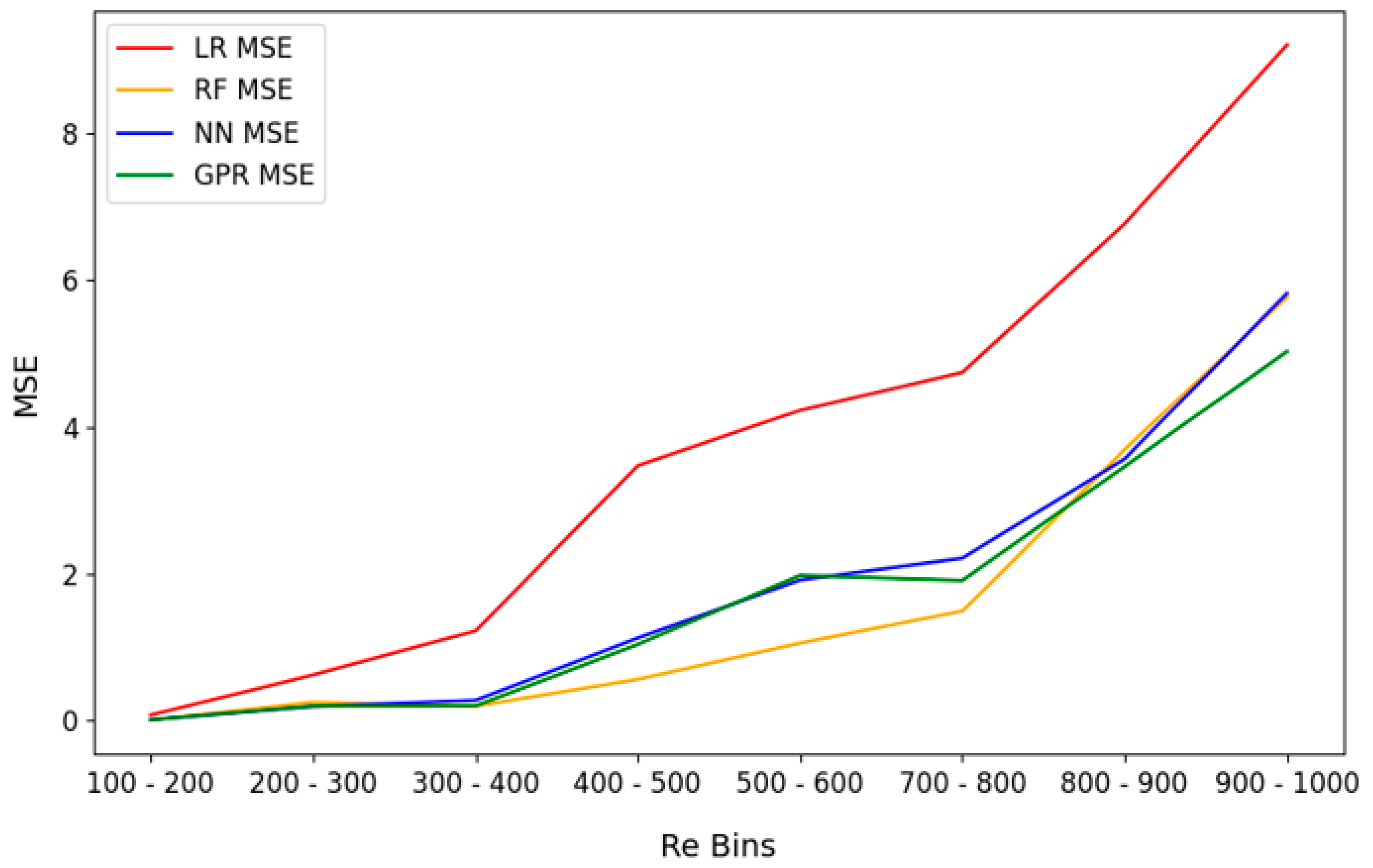
The neural network also performs well, closely trailing random forest in terms of accuracy. Although it shows slightly lower precision in predicting extreme conditions compared to random forest, its overall performance remains robust, especially when analyzing flow regimes characterized by moderate turbulence. These findings are further substantiated by the cross-validation results, where the mean squared error (MSE) of both random forest and neural network models remains consistently low across the entire range of Reynolds numbers, as illustrated in the cross-validation analysis observed in Figure 3. Random forest, in particular, demonstrates notable stability in its predictive capacity, maintaining low errors even as the Reynolds number approaches higher, more turbulent values.

An important part of the model interpretation involves understanding the impact of the key flow parameters—Reynolds number (Re), Richardson number (Ri), and the rotational speed of the cylinder (ω)—on the prediction of the average Nusselt number. Feature importance analysis is performed using SHAP (Shapley additive explanations, Microsoft Research: Redmond, WA, USA) value analysis, a method derived from cooperative game theory that helps to interpret complex machine-learning models by quantifying the contribution of each feature to the model’s predictions. SHAP values attribute an individual contribution to each feature by comparing the model’s output with and without that feature. It can be seen that Re consistently emerges as the feature with the highest average impact on model predictions, as depicted in Figure 4. This indicates the role of inertia in driving heat transfer within the cavity over the buoyancy and rotational effects.

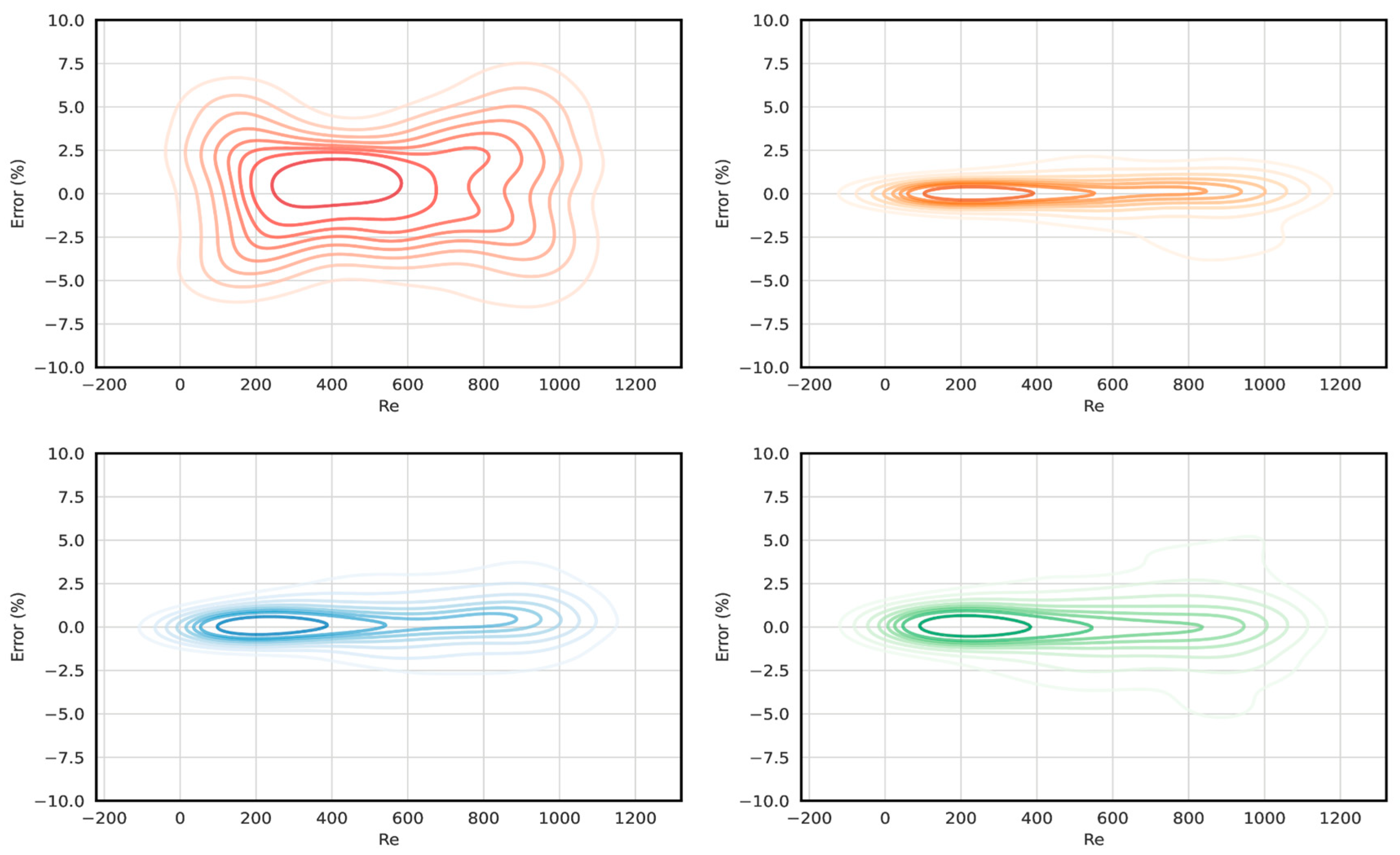
The error distribution across the different flow parameters is also tested to provide a better view into the strengths and weaknesses of the models. Among the key parameters affecting the predicted average Nusselt number (Nu), the Reynolds number (Re) consistently stands out as the most significant, as highlighted in the feature importance analysis. Given the dominant role of Re in the prediction process, we focus on the error contours for Re to examine the model’s accuracy under varying flow conditions.

Figure 5 illustrates the error contours for the Reynolds number across the tested ML models; the contours indicate that the random forest model (orange) and neural network (blue) show the lowest error values throughout the entire range of Re, demonstrating their ability to better capture the complex flow dynamics at higher Reynolds numbers. The Gaussian process regression model (green) follows closely, but with slightly higher errors in the upper Reynolds number range. Conversely, the linear regression model (red) exhibits the largest errors, particularly at higher Reynolds numbers, where the flow becomes more turbulent. This suggests that linear regression struggles to account for the nonlinear and chaotic nature of the flow at higher Re values, in contrast to more advanced models like random forest and neural network models, which manage to retain predictive accuracy even under these more challenging flow conditions.

4.2. Efficiency of Physics-Informed Neural Networks (PINN) in a Lid-Driven Cavity with a Rotating Cylinder

Physics-informed neural networks (PINNs) represent a groundbreaking approach that merges machine learning with physical laws to tackle complex problems. By embedding differential equations and boundary conditions directly into the training process, PINNs ensure that the solutions adhere to fundamental physical principles, such as the conservation of mass, momentum, and energy. This method is particularly advantageous in fields like flow and heat transfer. In fluid dynamics, PINNs can model intricate flow patterns by incorporating the Navier–Stokes equations, offering insights into phenomena ranging from aerodynamics to climate modeling. For heat transfer, PINNs solve problems related to temperature distribution and thermal conduction by integrating heat diffusion equations. The advantages of PINNs include their ability to handle complex and high-dimensional problems efficiently while ensuring physical consistency. They can significantly reduce the need for extensive data and computational resources, as the physical laws guide the learning process. However, the performance of PINNs is highly dependent on the choice of network architecture and hyperparameters, both of which play a crucial role in accurately capturing complex phenomena like flow dynamics. The architecture, including the number of layers, neurons, and activation functions, affects the network’s ability to model nonlinear behaviors, while the loss function must balance data-driven learning with the satisfaction of physical laws, such as conservation equations. Hyperparameters, such as the learning rate, batch size, and regularization, also significantly influence how well the model converges and generalizes. A poorly tuned learning rate can cause the model to oscillate or slow down convergence, while incorrect batch sizes or regularization terms may lead to overfitting or failure to capture critical flow features. Because PINNs must learn both from data and the governing physical equations, improper tuning can result in inaccurate representations of important flow dynamics, such as vortex formation or pressure gradients, especially in complex setups like a lid-driven cavity with a rotating cylinder. Therefore, optimizing the network architecture and hyperparameters is essential for the model to effectively generalize across different flow regimes, and failing to do so can lead to suboptimal or erroneous solutions.

In the study discussed, PINNs are tested on a heat transfer benchmark—specifically a buoyancy lid-driven thermal cavity with a rotating cylinder placed at the center of the cavity—to evaluate its performance. To the best knowledge of the present authors, this configuration never studied in the literature. As mentioned earlier, majority of the studies were focused on lid-driven flow and heat transfer inside a cavity. The fluid flow and thermal behavior inside a lid-driven cavity with a rotating cylinder are modeled using PINNs. The flow is analyzed for two Reynolds numbers, Re = 100 and Re = 1000, with comparisons made between actual data generated from computational fluid dynamics (CFD) simulations, PINN models trained with CFD data, and pure PINN models constructed without prior knowledge of data. The data-driven PINN model is constructed using pre-generated CFD data exported from Fluent, containing information on the velocity components u, v, pressure p, and temperature T fields at different Reynolds numbers. These data are used to train the neural network to predict flow and temperature fields with high accuracy. The neural network architecture consists of four hidden layers, each with 60 neurons, SiLU (sigmoid linear unit) is used as the activation function, which is known to improve convergence rates. The SiLU activation function is defined as follows:

SiLU(x) = x·σ(x)

(11)

where σ(x) is the sigmoid function. This choice of activation helps to capture the nonlinear dynamics of the system more effectively than the standard Tanh function. In this model, the loss function includes terms derived from the residuals of the continuity, momentum, and energy equations, which govern fluid flow and heat transfer. The training process involves optimizing the network parameters using the Adam optimizer, with the model trained for 10,000 epochs. PINNs combine data-based loss with the physics-informed loss by enforcing the residuals of the PDEs. A typical loss function, L, for PINNs can be expressed in general form as follows:

$$L=L_{data}+{\sum }_{i=1}^n{\lambda }_i{L}_{physicsi}$$

(12)

where L_data is the mean squared error (MSE) loss based on the difference between predicted and observed data (if available). L_physicsi is a loss term associated with the residuals of each governing equation (e.g., continuity, momentum, and energy). λ_i is a weighting factor for different physics terms.

Each residual loss term ensures that the model predictions satisfy the underlying physical laws:

$$L_{continuity}={‖\nabla ·\mathit{V}‖}^2$$

(13)

$$L_{momentum-x}={‖\mathit{V}·\nabla u+{\displaystyle \frac{1}{\rho }}{\displaystyle \frac{\partial p}{\partial x}}-\upsilon {\nabla }^{2}u‖}^2$$

(14)

$$L_{momentum-y}={‖\mathit{V}·\nabla v+{\displaystyle \frac{1}{\rho }}{\displaystyle \frac{\partial p}{\partial y}}-\upsilon {\nabla }^{2}v‖}^2$$

(15)

$$L_{energy}={‖\mathit{V}·\nabla T-\alpha {\nabla }^{2}T‖}^2$$

(16)

The loss function for this model is a combination of the mean squared error (MSE) between the predicted and actual values for each field, as well as a penalty term to enforce adherence to the no-slip condition on the surface of the rotating cylinder. This no-slip boundary condition ensures that the fluid velocity on the cylinder’s surface equals the tangential velocity imposed by the rotation of the cylinder, calculated as follows: v_θ = −ω × r, where ω is the angular velocity and r is the radial distance from the center of the cylinder. The total loss function is then expressed as follows:

L = L_u + L_v + L_p + L_T + λL_boundary

(17)

where L_u + L_v + L_p + L_T represent the MSE losses for the velocity components, pressure, and temperature fields, respectively, and L_boundary enforces the boundary conditions. The optimization process adjusts the neural network weights to minimize this loss over the specified number of epochs. Training data are interpolated onto a high-resolution grid, and a mask is applied to exclude points inside the rotating cylinder. In contrast to the data-driven approach, the second model employed a physics-based PINN method, often referred to as a purely physics-informed model. This approach does not rely on any pre-existing data but instead directly incorporates the governing Navier–Stokes and energy equations into the loss function, thus enforcing the physics of the system throughout the training process. The neural network architecture for this model consists of four layers with 50 neurons each, using the SiLU activation function, similar to the data-driven PINN model. Automatic differentiation is used to compute the necessary spatial derivatives of the predicted fields, allowing the model to enforce these physical laws. Additionally, the boundary conditions for the top wall (driven by velocity), bottom wall (stationary but thermally active), side walls, and the rotating cylinder are included as constraints in the loss function. The training process is carried out for 50,000 epochs, using the Adam optimizer and the total loss function in this model is defined as follows:

L_physics = L_continuity + L_momentum + L_energy + λL_boundary

(18)

where L_continuity ensures mass conservation, L_momentum corresponds to the momentum equations, and L_energy enforces the energy equation. The boundary loss term L_boundary is used for satisfying the boundary conditions at the walls and cylinder surface. The model is evaluated in the same Reynolds number regimes as the data-driven model.

The data-driven PINN model relies on the pre-existing CFD data to predict the flow and thermal fields. By training on actual data, the model implicitly learns to satisfy the governing equations and physical constraints, such as the continuity condition, without needing to explicitly compute the governing equations during training. This enables the model to focus on minimizing the error relative to the given data, which leads to faster training and more accurate predictions, particularly in cases where the flow behavior is intricate or nonlinear. On the other hand, the physics-based PINN model solves for the velocity components u, v, pressure p, temperature T, and stream function ψ by enforcing the governing Navier–Stokes and energy equations through automatic differentiation. The stream function ψ is used to ensure that the incompressibility condition ∇·u = 0 is automatically satisfied, simplifying the enforcement of the continuity equation. The momentum equations are expressed in terms of ψ, which governs the vorticity and streamlines of the flow, while the energy equation models the temperature distribution. The derivatives required for these equations are computed automatically through the network, and boundary conditions are applied as part of the loss function. This approach allows the physics-based PINN to predict flow behavior in situations where external data are unavailable, but it may become computationally more challenging when applied to more complex or turbulent flows, as it relies solely on the enforcement of physical laws through the loss function. The accuracy of PINNs is fundamentally tied to the precision of the embedded physical models. PINNs rely on the incorporation of governing physical laws, such as the Navier–Stokes equations for fluid flow or energy equation for thermal analysis, to guide the learning process alongside data. If these physical models are not accurately formulated or do not fully capture the complexities of the real-world system, the resulting predictions may deviate from actual behavior. This is particularly critical in complex flow scenarios, such as turbulent or multiphase flows, where even small inaccuracies in the representation of physical laws can lead to significant errors in the predicted velocity fields, temperature distributions, or pressure gradients. In cases involving complex geometries or boundary conditions, such as a lid-driven cavity with a rotating cylinder, any oversimplification or misrepresentation of the physical dynamics can cause the PINN to struggle in capturing phenomena like vortex formation or heat transfer patterns. Thus, the fidelity of the physical models embedded within PINNs directly constrains the network’s ability to make accurate and reliable predictions in real-world applications.

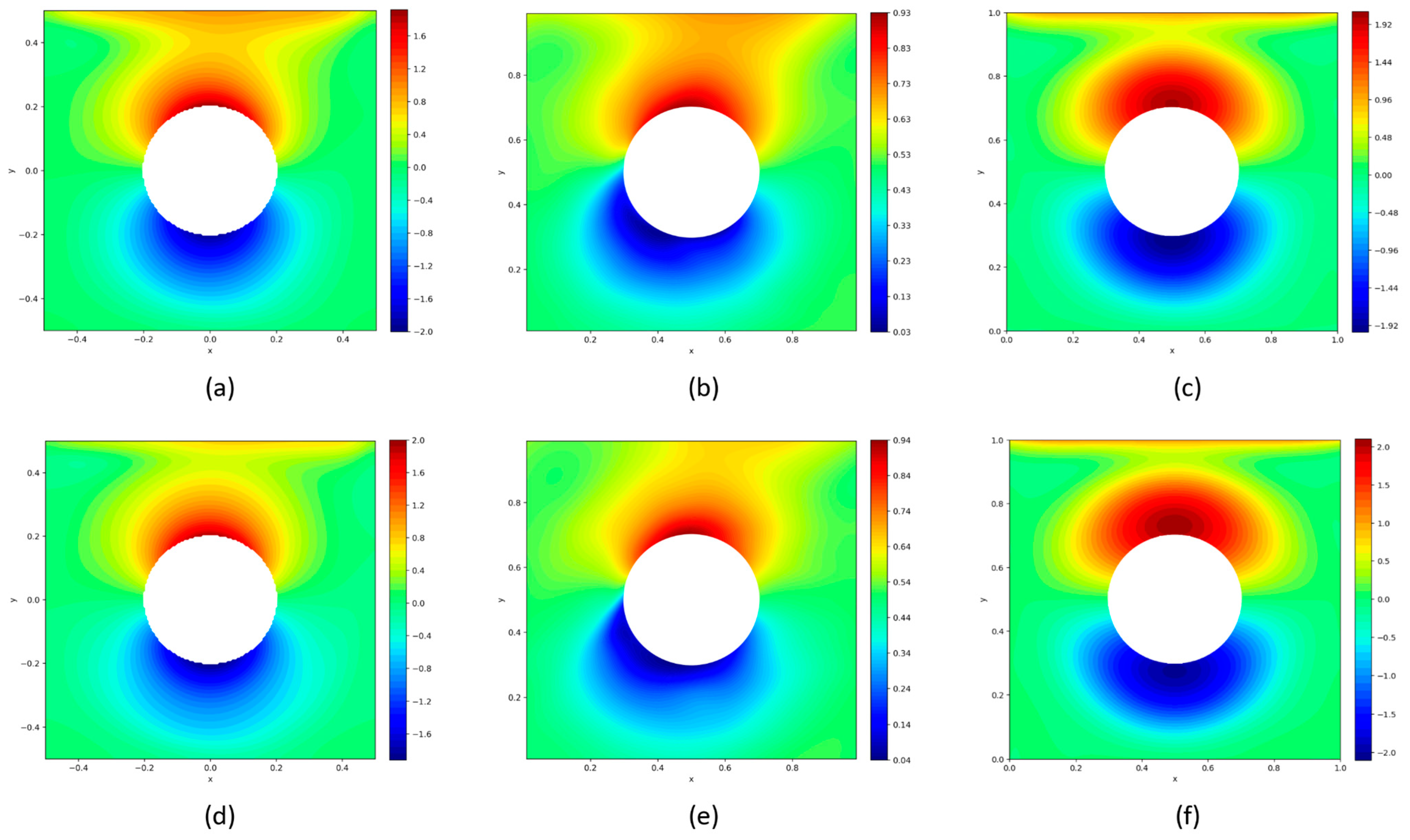
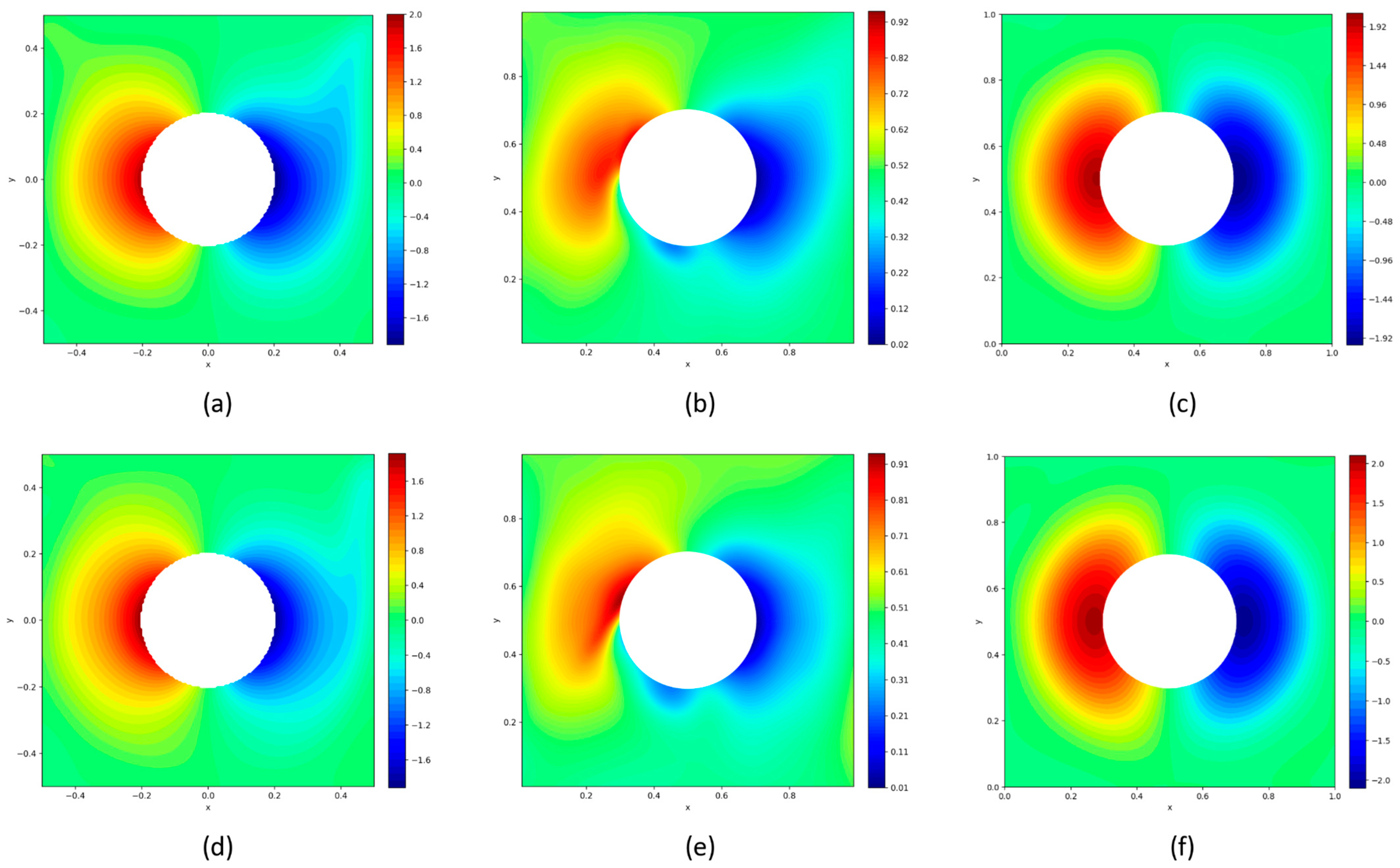
Both models are evaluated at the Reynolds numbers Re = 100 and Re = 1000, with the predictions for each field plotted and compared against the actual data generated from running the case using Fluent Ansys. Figure 6 shows the contours of the u-velocity for the lid-driven cavity with a rotating cylinder at its center, comparing with the actual data, the data-driven PINN results, and the physics-based PINN results for Re = 100 and Re = 1000, respectively. The actual data for Re = 100 and Re = 1000 demonstrate the expected flow behavior. At Re = 100 (Figure 6a), the flow is smooth, laminar, and symmetric around the rotating cylinder. The regions of positive and negative u-velocity are well-defined, with a clear recirculation zone above the cylinder (positive u) and a symmetric downward flow below (negative u). As the Reynolds number increases to Re = 1000 (Figure 6d), the flow becomes highly nonlinear, and the gradients of the u-velocity field become sharper, particularly around the cylinder. The recirculation zones tighten, indicating increased shear due to higher inertia forces. The data-driven PINN model results for both Re = 100 and Re = 1000 depicted in Figure 6b,e show a high degree of similarity to the actual data. At Re = 100, the recirculation zones and velocity transitions are captured accurately, with smooth gradients and proper representation of the laminar flow characteristics. At Re = 1000, the model continues to perform well in predicting the sharper gradients and tighter recirculation regions around the cylinder that arise due to the rotation of the cylinder. On the other hand, the results of the physics-based PINN model, shown in Figure 6c,f, correctly capture the general flow pattern but tend to produce overly smooth results, especially at Re = 1000. At Re = 100, the flow structure is largely correct, but the contours show a lack of irregularities that are present in the actual data and the data-driven model. This is even more pronounced at Re = 1000. This behavior can also be observed in the v-velocity analysis, as observed in Figure 7.

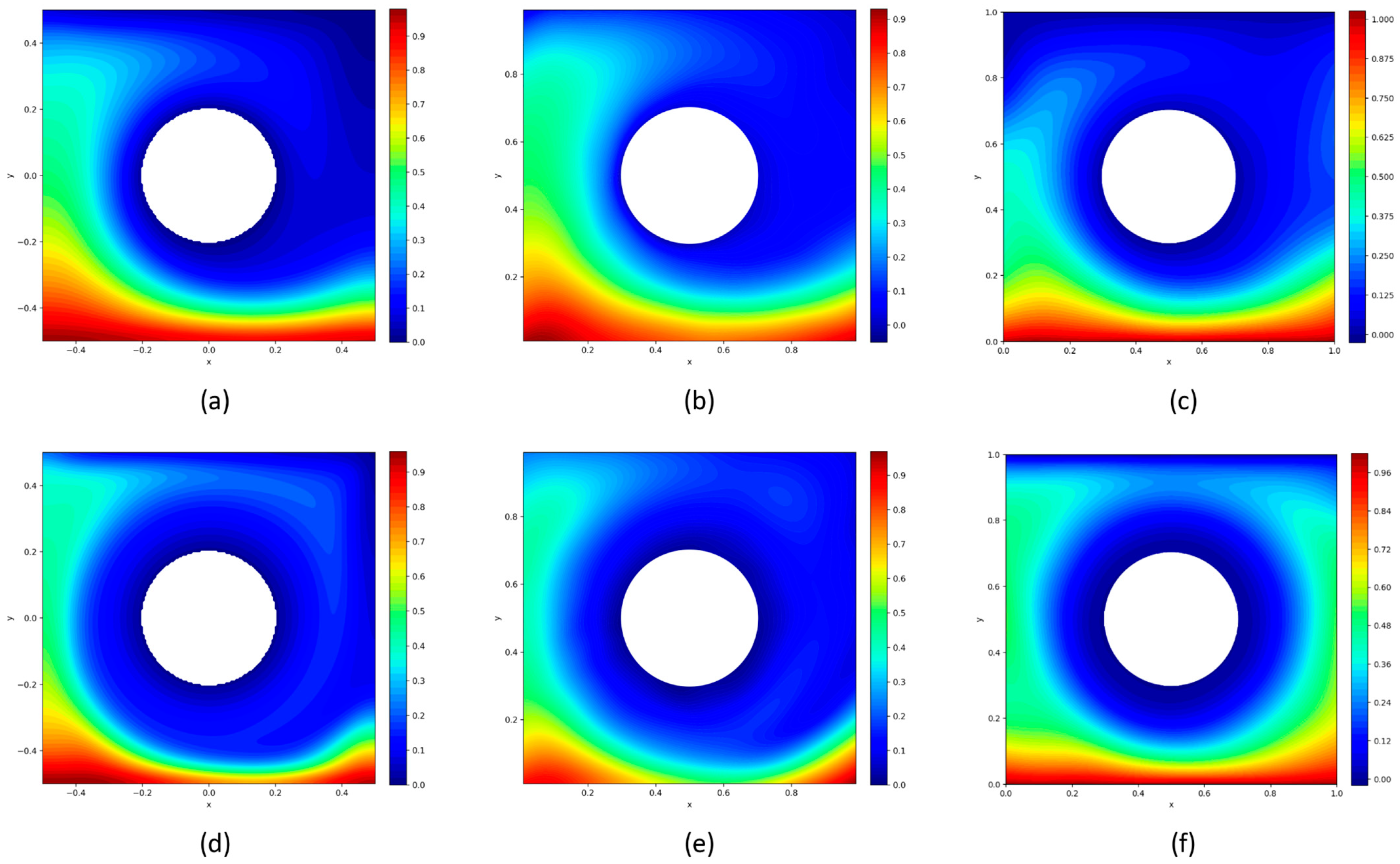
Figure 8 highlights the temperature distribution across the domain for both Re = 100 and Re = 1000, as previously mentioned, the lower wall is maintained at a hot temperature T_h = 1 and the upper wall at a cold temperature T_c = 0. The presence of a rotating cylinder in the center induces convective effects that influence the temperature gradients. At Re = 100, the actual data (Figure 8a) show a smooth transition from hot at the bottom to cold at the top, with mild rotational influence around the cylinder. The data-driven PINN (Figure 8b) accurately replicates this thermal behavior. The physics-based PINN (Figure 8c), while generally following the same trend, produces a slightly smoother temperature field, indicating that it fails to capture the localized thermal effects of the rotation as precisely as the data-driven model. At Re = 1000, the actual data (Figure 8d) reveal sharper temperature gradients near the hot wall due to increased convection, with the rotating cylinder further disturbing the temperature field. The data-driven PINN (Figure 8e) closely mimics these sharper gradients and rotational effects, effectively representing the complex convective flow. However, the physics-based PINN (Figure 8f) once again produces a more uniform temperature field and struggles to accurately capture the enhanced convection and rotational disturbances.

This difference in performance can be further observed in the MAE and physics loss results shown in

Table 2. Mean absolute error (MAE) and physics loss for data-driven and physics-based PINN models at Re = 100 and Re = 1000.

Model	MAE Re = 100	Physics Loss Re = 100	MAE Re = 1000	Physics Loss Re = 1000
Data-driven PINN	3.16 × 10−2	8.68 × 10−1	3.9 × 10−2	1.304
Physics-based PINN	5.24 × 10−1	3.03 × 10−2	1.57	2.56 × 10−2

. It is shown that the data-driven PINN achieves a significantly lower MAE at both Reynolds numbers, while the physics-based PINN exhibits much lower physics loss at both Reynolds numbers. This can be attributed to the model directly enforcing the governing equations through its loss function, which leads to higher adherence to physical laws. However, the higher MAE indicates that this strict adherence leads to less accurate predictions, particularly at higher Reynolds numbers, where the flow becomes more turbulent and difficult to resolve. In summary, the study emphasizes the challenges of achieving both convergence and stability during the training process, particularly when accounting for the expanded parameter space introduced by varying the rotation speeds, lid-driven speeds, and directions of the cylinder. As the complexity of the flow dynamics increases, it becomes more difficult for the model to generalize effectively. This increased complexity often results in overtraining, where the model fits the training data with high accuracy but fails to perform well on unseen or new data. The difficulty in balancing the learning process and ensuring the model adapts to a broad range of conditions without sacrificing predictive accuracy represents a critical limitation in machine-learning applications for complex flow and heat transfer problems.

5. Conclusions

This study highlights the role of machine learning-based predictions in enhancing the understanding of heat transfer in lid-driven cavities, a key issue in computational fluid dynamics (CFD). Lid-driven cavities involve fluid motion driven by one moving wall, and the study focused on developing machine-learning regression models to analyze discrepancies between predicted and actual average Nusselt numbers. Physics-informed neural networks (PINNs) were also utilized to model flow and thermal behavior at varying Reynolds numbers, comparing results from CFD simulations, PINNs trained with CFD data, and purely theoretical PINNs without prior data input. The random forest model emerged as the most stable and accurate, maintaining low error rates even at higher Reynolds numbers, outperforming the other models. Flow and thermal behavior were found to heavily depend on the type of PINN used. The data-driven PINN showed lower mean average errors by incorporating CFD data, adapting to the nonlinearities and turbulence present in real-world flows. In contrast, the physics-based PINN, which strictly followed theoretical principles, exhibited lower physics loss but produced smoother, more idealized solutions, failing to capture complex flow behavior at higher Reynolds numbers.

The novelty of this study lies in its comprehensive comparison of machine-learning techniques, particularly PINNs, in predicting complex heat transfer behavior, bridging the gap between traditional CFD and advanced machine-learning models. The use of PINNs, combined with CFD data, demonstrated a significant improvement in capturing real-world flow dynamics. This contribution offers a new approach to enhancing the accuracy and efficiency of CFD simulations, particularly for complex systems where high Reynolds numbers introduce nonlinearities. To mitigate the limitations of PINNs, several improvements can be implemented. Physics-data combined machine learning and parametric reduced-order models (ROMs) can help to accelerate convergence and improve generalization by integrating real-world data. XPINNs extend PINNs by dividing the domain into subdomains, enabling better boundary handling and scalability. Additionally, combining physics and data through neural networks and employing multi-fidelity approaches can reduce training instability, improve accuracy, and enhance performance in complex, real-world applications.

References

1. Khanafer, K.; Chamkha, A.J. Mixed convection flow in a lid-driven enclosure filled with a fluid-saturated porous medium. Int. J. Heat Mass Transf. 1998, 42, 2465–2481. [Google Scholar] [CrossRef]
2. Khanafer, K.; Vafai, K. Double-diffusive mixed convection in a lid-driven enclosure filled with a fluid-saturated porous medium. Numer. Heat Transf. A 2002, 42, 465–486. [Google Scholar] [CrossRef]
3. Khanafer, K.; AlAmiri, A.; Pop, I. Numerical simulation of unsteady mixed convection in a driven cavity using an externally excited sliding lid. Eur. J. Mech. B Fluids 2007, 26, 669–687. [Google Scholar] [CrossRef]
4. Iwatsu, R.; Hyun, J.M.; Kuwahara, K. Mixed convection in a driven cavity with a stable vertical temperature gradient. Int. J. Heat Mass Transf. 1993, 36, 1601–1608. [Google Scholar] [CrossRef]
5. Al-Amiri, A.; Khanafer, K.; Bull, J.; Pop, I. Effect of sinusoidal wavy bottom surface on mixed convection heat transfer in a lid-driven cavity. Int. J. Heat Mass Transf. 2007, 50, 1771–1780. [Google Scholar] [CrossRef]
6. Khanafer, K.; Aithal, S.M. Mixed convection heat transfer in a lid-driven cavity with a rotating circular cylinder. Int. Commun. Heat Mass Transf. 2017, 86, 131–142. [Google Scholar] [CrossRef]
7. Khanafer, K.; Aithal, S.M.; Vafai, K. Mixed convection heat transfer in a differentially heated cavity with two rotating cylinders. Int. J. Therm. Sci. 2019, 135, 117–132. [Google Scholar] [CrossRef]
8. Ghaddar, N.K. Natural convection over rotating cylindrical heat source in an enclosure. J. Thermophys. Heat Transf. 1996, 10, 303–311. [Google Scholar] [CrossRef]
9. Liao, C.-C.; Lin, C.-A. Mixed convection of a heated rotating cylinder in a square enclosure. Int. J. Heat Mass Transf. 2014, 72, 9–22. [Google Scholar] [CrossRef]
10. Soori, M.; Arezoo, B.; Dastres, R. Artificial intelligence, machine learning and deep learning in advanced robotics, a review. Cogn. Robot. 2023, 3, 54–70. [Google Scholar] [CrossRef]
11. Beam, A.; Kohane, I. Big Data and Machine Learning in Health Care. JAMA 2018, 319, 1317–1318. [Google Scholar] [CrossRef] [PubMed]
12. Brunton, S.; Noack, B.; Koumoutsakos, P. Machine learning for fluid mechanics. Annu. Rev. Fluid Mech. 2020, 52, 477–508. [Google Scholar] [CrossRef]
13. Joss, L.; Müller, E. Machine learning for fluid property correlations: Classroom examples with MATLAB. J. Chem. Educ. 2019, 96, 697–703. [Google Scholar] [CrossRef]
14. Brenner, M.P.; Eldredge, J.D.; Freund, J.B. Perspective on machine learning for advancing fluid mechanics. Phys. Rev. Fluids 2019, 4, 100501. [Google Scholar] [CrossRef]
15. Pandey, S.; Schumacher, J.; Sreenivasan, K.R. A perspective on machine learning in turbulent flows. J. Turbul. 2020, 21, 567–584. [Google Scholar] [CrossRef]
16. Kwon, B.; Ejaz, F.; Hwang, L. Machine learning for heat transfer correlations. Int. Commun. Heat Mass Transf. 2020, 116, 104694. [Google Scholar] [CrossRef]
17. Zohora, F.; Akter, F.; Haque, A.; Chowdhury, N.; Haque, M. A novel pin finned structure-embedded microchannel heat sink: CFD-data driven MLP, MLR, and XGBR machine learning models for thermal and fluid flow prediction. Energy 2024, 307, 132646. [Google Scholar] [CrossRef]
18. Hashemi, Z.; Gholampour, M.; Wu, M.; Liu, T.; Liang, C.; Wang, C. A physics-informed neural networks modeling with coupled fluid flow and heat transfer–Revisit of natural convection in cavity. Int. Commun. Heat Mass Transf. 2024, 157, 107827. [Google Scholar] [CrossRef]
19. Chu, H.; Ji, T.; Yu, X.; Liu, Z.; Rui, Z.; Xu, N. Advances in the application of machine learning to boiling heat transfer: A review. Int. J. Heat Fluid Flow 2024, 108, 109477. [Google Scholar] [CrossRef]
20. Selimefendigil, F.; Öztop, H. Estimation of the mixed convection heat transfer of a rotating cylinder in a vented cavity subjected to nanofluid by using generalized neural networks. Numer. Heat Transf. Part A Appl. Int. J. Comput. Methodol. 2014, 65, 165–185. [Google Scholar] [CrossRef]
21. Tizakast, Y.; Kaddiri, M.; Lamsaadi, M.; Makayssi, T. Machine Learning based algorithms for modeling natural convection fluid flow and heat and mass transfer in rectangular cavities filled with non-Newtonian fluids. Eng. Appl. Artif. Intell. 2023, 119, 105750. [Google Scholar] [CrossRef]
22. Larrañaga, A.; Martínez, J.; Míguez, J.L.; Porteiro, J. Robust optimization of heat-transfer-enhancing microtextured surfaces based on machine learning surrogate models. Int. Commun. Heat Mass Transfer. 2024, 151, 107218. [Google Scholar] [CrossRef]
23. Costa Rocha, P.A.; Johnston, S.J.; Oliveira Santos, V.; Aliabadi, A.A.; Thé, J.V.G.; Gharabaghi, B. Deep Neural Network Modeling for CFD Simulations: Benchmarking the Fourier Neural Operator on the Lid-Driven Cavity Case. Appl. Sci. 2023, 13, 3165. [Google Scholar] [CrossRef]
24. Ranade, R.; Hill, C.; Pathak, J. DiscretizationNet: A machine-learning based solver for Navier–Stokes equations using finite volume discretization. Comput. Methods Appl. Mech. Eng. 2021, 378, 113722. [Google Scholar] [CrossRef]
25. Sreerag, E.; Balaji, S. Feasibility study of using Machine Learning to accelerate CFD solvers. In Proceedings of the 4th International Conference on Fluid Flow and Thermal Science (ICFFTS’23), Lisbon, Portugal, 7–9 December 2023. [Google Scholar]
26. Bai, X.-d.; Wang, Y.; Zhang, W. Applying physics informed neural network for flow data assimilation. J. Hydrodyn 2020, 32, 1050–1058. [Google Scholar] [CrossRef]
Figure 1. Schematic diagram of the problem under consideration.
Energies 17 05220 g001
Figure 2. Scatter plots of predicted vs. actual Nusselt number for (a) linear regression (red), (b) random forest (orange), (c) neural network (blue), and (d) Gaussian process regression (green).
Energies 17 05220 g002
Figure 3. Cross−validation MSE for machine-learning models across Reynolds numbers: Linear regression (red), random forest (orange), neural network (blue), and Gaussian process regression (green).
Energies 17 05220 g003
Figure 4. SHAP value analysis for feature importance of the Reynolds number (Re), Richardson number (Ri), and rotational speed (ω) in predicting the Nusselt number.
Energies 17 05220 g004
Figure 5. Error contours of the Reynolds number (Re) for the predicted Nusselt number across different machine-learning models: linear regression (red), random forest (orange), neural network (blue), and Gaussian process regression (green).
Energies 17 05220 g005
Figure 6. u-velocity distribution at Re = 100 (ac) and Re = 1000 (df) of the actual data (a,d), data-driven PINN (b,e), and physics-based PINN (c,f).
Energies 17 05220 g006
Figure 7. v-velocity distribution at Re = 100 (ac) and Re = 1000 (df) of the actual data (a,d), data-driven PINN (b,e), and physics-based PINN (c,f).
Energies 17 05220 g007
Figure 8. Temperature profile at Re = 100 (ac) and Re = 1000 (df) of the actual data (a,d), data-driven PINN (b,e), and physics-based PINN (c,f).
Energies 17 05220 g008