Article

Machine Learning and Cointegration for Wind Turbine Monitoring and Fault Detection: From a Comparative Study to a Combined Approach

1
IBM Poland, Armii Krajowej 18, 30-150 Krakow, Poland
2
Department of Robotics and Mechatronics, Faculty of Mechanical Engineering and Robotics, AGH University of Krakow, Al. Mickiewicza 30, 30-059 Krakow, Poland
*
Author to whom correspondence should be addressed.
Energies 2024, 17(20), 5055; https://doi.org/10.3390/en17205055
Submission received: 11 September 2024 / Revised: 8 October 2024 / Accepted: 9 October 2024 / Published: 11 October 2024
(This article belongs to the Section A3: Wind, Wave and Tidal Energy)

Abstract

:
Data-driven models have become powerful tools for structural and condition monitoring of engineering systems, particularly wind turbines. This paper presents a comparative analysis of common machine learning (ML) algorithms (artificial neural networks, linear regression, random forests, and gradient boosting) and a cointegration-based approach for fault detection using Supervisory Control and Data Acquisition (SCADA) data. While ML models offer early fault prediction, the cointegration method is simpler, requires less training data, and has lower computational costs. However, it is less effective for early detection. To balance these trade-offs, we propose a cascading monitoring framework, where the ML model provides long-term predictions (outer monitoring process) and the cointegration model offers short-term verification (inner monitoring process). The cointegration model serves to confirm anomalies flagged by the ML model. By combining both models in a cascade structure, the system reduces the risk of false alarms triggered by uncertainties in the ML model alone. Furthermore, the short-term cointegration-based prediction model helps pinpoint immediate risks and mitigate the issue of prolonged downtime. This combination enhances both accuracy and reliability, as demonstrated through testing on a five-year SCADA dataset from a commercial wind turbine with a known gearbox fault.

1. Introduction

Wind power has emerged as a promising alternative to traditional fossil fuel-based sources of electricity generation due to its potential to produce clean and low-carbon energy. In 2023, the worldwide newly installed wind power capacity reached a record of 117 GW, contributing to a cumulative installed global capacity of 1023 GW. At the current rate, the wind industry expects to hit 2 TW before 2030 [1]. Wind turbines, being intricate systems, function in harsh environmental conditions, thereby encountering various challenges and difficulties in Operation and Maintenance (O&M) tasks [2]. Failures in crucial components of wind turbines, such as generators and gearboxes, can lead to costly downtime and maintenance, negatively impacting their performance and lifespan [3]. Therefore, in recent years, there has been an increasing demand for developing effective condition monitoring and anomaly detection methods for both onshore and offshore wind turbines. Many schemes have been proposed in recent years. An overview of the different strategies can be found in [2,3,4]. One of the most common solutions is to detect abnormal behaviour in wind turbines as early as possible before critical failures occur [3,5]. Then, the malfunction can be corrected more rapidly and without leading to serious damage to principal turbine subsystems such as the main bearing or gearbox.
Supervisory Control and Data Acquisition (SCADA) systems are commonly installed in the majority of wind farms. Sensors placed in different parts of the wind turbine are responsible for collecting SCADA data for various process parameters, for example, the wind speed, generator and rotor speed, subsystem temperature, pressure, voltage, current, power characteristics, energy conversion process parameters, and alarm status. The data are obtained through statistics of recorded signals, such as minimum and maximum values, mean values, standard deviation, root mean square, etc. The data collected by these systems offer significant advantages in terms of large scale, cost-effectiveness, and extensive monitoring coverage. SCADA data contain valuable information about the performance and health of wind turbines, which can be analysed to identify potential faults and predict maintenance requirements [4]. Therefore, SCADA-based solutions have been considered the most cost-efficient option for implementing intelligent O&M strategies for wind turbines, as reported in the literature [4,5,6,7,8].
In recent years, there has been a growing interest in the development of advanced statistical methods and machine learning (ML)-based techniques for analysing SCADA data to predict potential faults and maintenance requirements, thereby improving the reliability and efficiency of wind turbines. As reported in a recent survey [9], the most commonly used ML models for wind turbine condition monitoring include artificial neural network (ANN), Support Vector Machine (SVM), and Decision Tree (DT). In [10], an ML-based approach was introduced, employing Gaussian processes to predict the edge frequencies of a wind turbine’s blade. Consequently, this method allows for the assessment of when a blade begins to exhibit altered behaviour. A data-mining approach using ANNs was developed in [11] to model the behaviour of key components, such as the gearbox and generator, in order to predict operational anomalies of the wind turbine. The work in [12] developed a condition monitoring system for wind turbines by integrating ANNs with additional data post-processing analysis to ensure that the ANN models are trained on the data accurately representing the normal operating conditions of the wind turbine. The method was effectively applied in case studies involving gearbox failures in wind turbines. The research in [13] proposed a condition monitoring method using a Recurrent Neural Network (RNN), which, due to its recurrent structure, was able to efficiently learn the long-time temporal dependencies between various wind turbine parameters. The study in [14] proposed a method combining the Convolutional Neural Network (CNN) and the Long Short-Term Memory (LSTM) network together with an attention mechanism for fault detection in wind turbines. Another work employing CNNs for fault detection based on wind turbine SCADA data was reported in [15]. The authors demonstrated that the CNN model exhibited superior performance in detecting faults in wind turbines, achieving earlier detection and higher accuracy and robustness of prediction compared to conventional fully connected neural networks. Deep Neural Networks (DNNs) were investigated in [16,17] for anomaly detection and fault analysis. Because of their multilayer learning characteristic for input features, DNN models demonstrated superior performance, enabling precise anomaly detection of various turbine components. Lately, numerous sophisticated ML techniques have emerged for diagnosing faults in wind turbine power plants, as reported in recent studies [18,19,20,21,22,23,24]. It should also be mentioned that advanced ML algorithms and deep transfer learning have been successfully applied in other industrial applications, such as the classification of failure modes in insulated-gate bipolar transistor (IGBT) modules [25] and battery applications [26,27].
Although ML-based algorithms are widely used for wind turbine condition monitoring and fault detection, they present some drawbacks, including complexity, the need for large training datasets, lengthy training times, and high computational costs [3,9]. Hence, simpler and more computationally efficient approaches have been investigated in recent years. A feasible solution has been to explore the applicability of statistical techniques originating from econometrics and statistics. Consequently, many statistical methods have been adapted for wind turbine health monitoring and fault assessment. Some representative examples include multiway principal component analysis [6], least squares support vector regression [28], change-point detection [29,30,31], cumulative sum computation-based methods [32,33], and the Wilcoxon rank-sum test-based method [34].
In the past few years, the cointegration theory, originally established within the field of econometrics and statistics [35,36], has found its potential applications in the domain of structural damage detection [37,38,39,40,41,42,43,44], as well as for condition monitoring and fault detection of wind turbines, as reported in the literature. In [45,46,47], a cointegration-based condition monitoring solution was investigated and validated using a SCADA dataset obtained from a 2 MW wind turbine drivetrain under varying environmental and operational conditions. The dataset involved a gearbox fault event. The results confirmed the effectiveness of the proposed method in removing nonlinear data trends, ensuring continuous monitoring of the wind turbine, and reliably identifying the gearbox fault. Another method based on cointegration was developed in [48] for efficiently monitoring the anomalous condition of the generator and gearbox, enabling early detection of faults. In [49,50], SCADA data recorded from a 1.5 MW wind turbine operating under the influence of environmental and operational fluctuations were used to develop a cointegration model aimed at identifying a number of gearbox fault data. In the study [51], the cointegration analysis was applied to analyse vibration data in order to detect damage in a wind turbine blade under the impact of environmental conditions. The results indicated that cointegration could identify the presence of damage even in situations where direct discrimination between damage and environmental factors was challenging. The work in [52] introduced a Bayesian multivariate cointegration technique for vibration-based damage detection with the purpose of identifying the gradual deterioration in a wind turbine blade. A study on cointegration for wind turbine monitoring and fault detection was carried out in [53], in which two different sets of SCADA data were used to train the cointegration model. Interestingly, despite using two different training datasets, the cointegration process created two identical residuals, which could successfully monitor the wind turbine and accurately detect the fault at the early stage. Recently, the work in [54] proposed a monitoring method—based on a combination of the sparse cointegration analysis and independent component analysis—to detect faults in wind turbines. More recently, a method based on the frequency domain decomposition and cointegration analysis was developed in [55] for damage assessment of offshore platforms subject to wind and wave loads. Given the importance of monitoring and removing nonlinear trends that manifest between wind turbine parameters, as well as in the relationships between these parameters and environmental factors such as wind speed and air temperature, the study in [56] developed a homoscedastic nonlinear cointegration approach for operational state monitoring and fault detection of wind turbines.
In summary, ML- and cointegration-based approaches have been employed for operational state monitoring and fault detection in wind turbines using SCADA data. A common point in both approaches involves developing normal behaviour models for key turbine components, as discussed in [57,58,59,60,61,62]. Fault or anomaly detection is then based on the deviations between the predicted model outputs and the actual measured values. However, their own advantages and disadvantages have not yet been thoroughly investigated and compared. Hence, this study contributes to the existing literature by conducting an experimental investigation and comparative analysis between common machine learning algorithms (including artificial neural network, linear regression, random forest, and gradient boosting) and the cointegration-based method. The objective is to predict or detect a failure in the turbine gearbox at the earliest possible stage. A five-year SCADA dataset collected from a commercial wind turbine (from 1 January 2013 to 13 January 2018) experiencing a gearbox fault was utilised as a test case to evaluate and compare ML and cointegration models. ML algorithms outperform the cointegration-based monitoring solution in terms of providing early indications of gearbox faults. However, the cointegration-based approach offers advantages in simplicity, requiring less training data and lower computational costs. The findings of this study will be helpful for the potential users of both approaches in the future.
The remainder of this paper is organised as follows: Section 2 gives a brief introduction to ML algorithms, including artificial neural network, linear regression, random forest, and gradient boosting, along with an overview of cointegration theory. Section 3 presents the wind turbine SCADA dataset used in this study and outlines the data preprocessing procedure. Results of the condition monitoring and fault detection using ML models and cointegration analysis are reported in Section 4 and Section 5, respectively. Section 6 discusses a proposal for combining ML and cointegration for wind turbine monitoring. Finally, Section 7 concludes the paper with summaries and suggestions for future work.

2. Background

2.1. Machine Learning Algorithms

ML is a field of Artificial Intelligence (AI) dedicated to algorithms capable of imitating human behaviour by building a mathematical model based on available data and improving performance during a training process. ML methods are often used in a regression task to estimate the relationship between dependent (output) and independent (input) variables. Common performance metrics used to evaluate the effectiveness of an ML model are as follows: the coefficient of determination (R2 score), the Mean-Squared Error (MSE), and the Mean Absolute Error (MAE). A brief introduction to the ML algorithms used in this study is provided below. For further details, readers are referred to [63].
ANN is a computational model that includes a collection of nodes (neurons) organised into layers, which is capable of approximating a nonlinear model by modifying its internal structure. The most popular type of ANN is the Multilayer Perceptron (MLP), which consists of an input layer, an output layer, and one or more hidden layers between the two formers. MLP is a kind of feed-forward ANN, as the output of each processing element does not affect that node itself. The training process of an MLP, by means of the optimisation of its weights, is often conducted by using the backpropagation algorithm, which minimises the error between a network’s estimated outputs and actual outputs.
Linear Regression (LR) is one of the simplest types of regression estimators, which tries to find a relationship between independent and dependent variables, assuming that it is linear. A multivariate LR model is represented by the following formula:
y = β 0 + β 1 x 1 + β 2 x 2 + + β n x n + ϵ
where y is a targeted variable, x is input variables, β is linear coefficients, and ε is an error. The estimation of coefficients is usually conducted by using either the gradient descent or the Ordinary Least Squares (OLS) method, which tries to minimise the sum of squared residuals.
Random Forest (RF) is an algorithm that is an assembly of DTs combined to form an aggregated estimate. In an RF model, DTs are created by splitting each node using the best feature from a subset of randomly chosen predictors. This is contrary to typical DTs, where nodes are divided based on the most important feature among all. Adding this randomness results in better performance compared to other ML methods and provides robustness against the overfitting problem.
Gradient Boosting Tree (GBT) is an ensemble ML technique where decision trees are sequentially built to correct the errors of the previous trees. Firstly, a single DT is created that makes predictions; then, the algorithm iteratively builds more—usually shallow—trees, which are fitted to the residuals of the former ones by calculating the gradient of the loss function. Each tree’s contribution to the final prediction is weighted based on its performance. GBTs can handle complex nonlinear relationships and are robust to outliers. However, they are sensitive to hyperparameters and require careful training to prevent overfitting.

2.2. Cointegration Theory

Let Y t = ( y 1 t , y 2 t , , y n t ) T denote an ( n × 1 ) vector of nonstationary time series. This n-dimension vector is said to be linearly cointegrated if there exists a vector β = ( β 1 , β 2 , , β n ) T such that
β T Y t = β 1 y 1 t + β 2 y 2 t + + β n y n t
is stationary. The linear combination, denoted as u t = β T Y t + c , where c is a constant, is called a cointegration residual, representing a long-run equilibrium relationship between the cointegrated time series [64]. The vector β is known as the cointegrating vector. In practice, a normalised cointegrating vector β , with the form given in Equation (3), is often used.
β = ( 1 , β 2 , , β n ) T
Using this normalised cointegrating vector, the cointegration relationship in Equation (2) will have a new form:
β T Y t = y 1 t β 2 y 2 t β n y n t
Then, the forming of a cointegration residual (i.e., u t = β T Y t + c ) can be understood as projecting n vectors of time series in Y t on a normalised cointegrating vector β .
So, the key issue of the cointegration method is to estimate appropriate normalised cointegrating vectors to create stationary residuals. Johansen’s cointegration method [33], a sequential procedure based on the maximum likelihood estimation procedure, is mostly used for this purpose. The underlying theory of this method is complex and thus not presented here. For more theoretical details, potential readers are recommended to the original work [33], with a simpler description available in [34,35]. In this work, Johansen’s cointegration procedure was employed using the Econometrics Toolbox [65] to estimate the normalised cointegrating vectors.

3. Wind Turbine SCADA Data

3.1. Data Description

The SCADA data used in the study comes from an operating wind turbine (model MM82, manufactured by Senvion SE in Germany, with a rated power of 2 MW), which is located at the La Houte Bourne wind farm in France [66]. In total, 34 process parameters were monitored and recorded by the SCADA system at 10-min intervals from 1 January 2013 to 13 January 2018, resulting in a 5-year dataset with 264,528 data samples recorded for each parameter. The dataset includes many parameters, such as wind speed, absolute wind direction, outdoor temperature, rotor bearing temperature, gearbox bearing temperature, generator bearing temperature, gearbox oil sump temperature, generator speed, generated power, torque, grid voltage, grid frequency, vane position, pitch angle, and more. For each parameter, the average value, standard deviation, maximum, and minimum values were collected at every interval. In this study, only the average values of the parameters were used for the analysis.

3.2. Data Preprocessing

The collected SCADA data were required to be preprocessed to make it suitable for use with ML methods and the cointegration process. The aim was to remove corrupted and redundant information that could affect the performance of the models. The preprocessing procedure for SCADA data comprises three steps, namely corrupted data removal, dimensionality reduction, and data scaling, which are explained in the following.
Before performing the data preprocessing, we carefully selected an appropriate number of data samples from the entire available dataset. The purpose of this task is to ensure the best quality of the training data for ML models and cointegration analysis. It should be noted that since the wind turbine under investigation is associated with a 5-year dataset, we have plenty of data to perform this selection. In this work, the choice of data was made based on the time series analysis of the target variable—the gearbox bearing temperature (plotted in Figure 1)—as well as the analysis of its value distribution (shown in Figure 2). Consequently, the data used in this paper have been selected in such a way that it consists of four different time periods: from 1 April 2013 to 31 May 2013, from 1 August 2013 to 31 October 2013, from 1 January 2014 to 30 September 2014, and from 1 March 2016 to 30 September 2016. This formed a total of 21 months of data, from which 85% and 15% of the samples were chosen for training and testing the models, respectively. Moreover, the selected data was further filtered to include only temperature values within the range of 29 to 76 °C, as illustrated in Figure 2. This range was chosen because most of the samples fall within it. In addition, we assume that the temperature range under consideration represents the normal operating conditions for the wind turbine. It should be noted that the specified range of bearing temperature was selected specifically for the turbine under investigation. In general, the upper and lower limits for bearing temperature should be analysed and properly estimated on a case-by-case basis, depending on the site and turbine brand.
The first step in the data preprocessing (i.e., removal of corrupted data) was to remove both missing and corrupted values. The former may deteriorate the accuracy of prediction, and there is no need to replace them as there is enough data available. In the end, there were only 12 samples that were ‘NaNs’ (for the analysed periods). In the case of the latter, samples that contained unphysical values, for instance, negative wind speed, were also removed as they indicated only errors in sensor measurements.
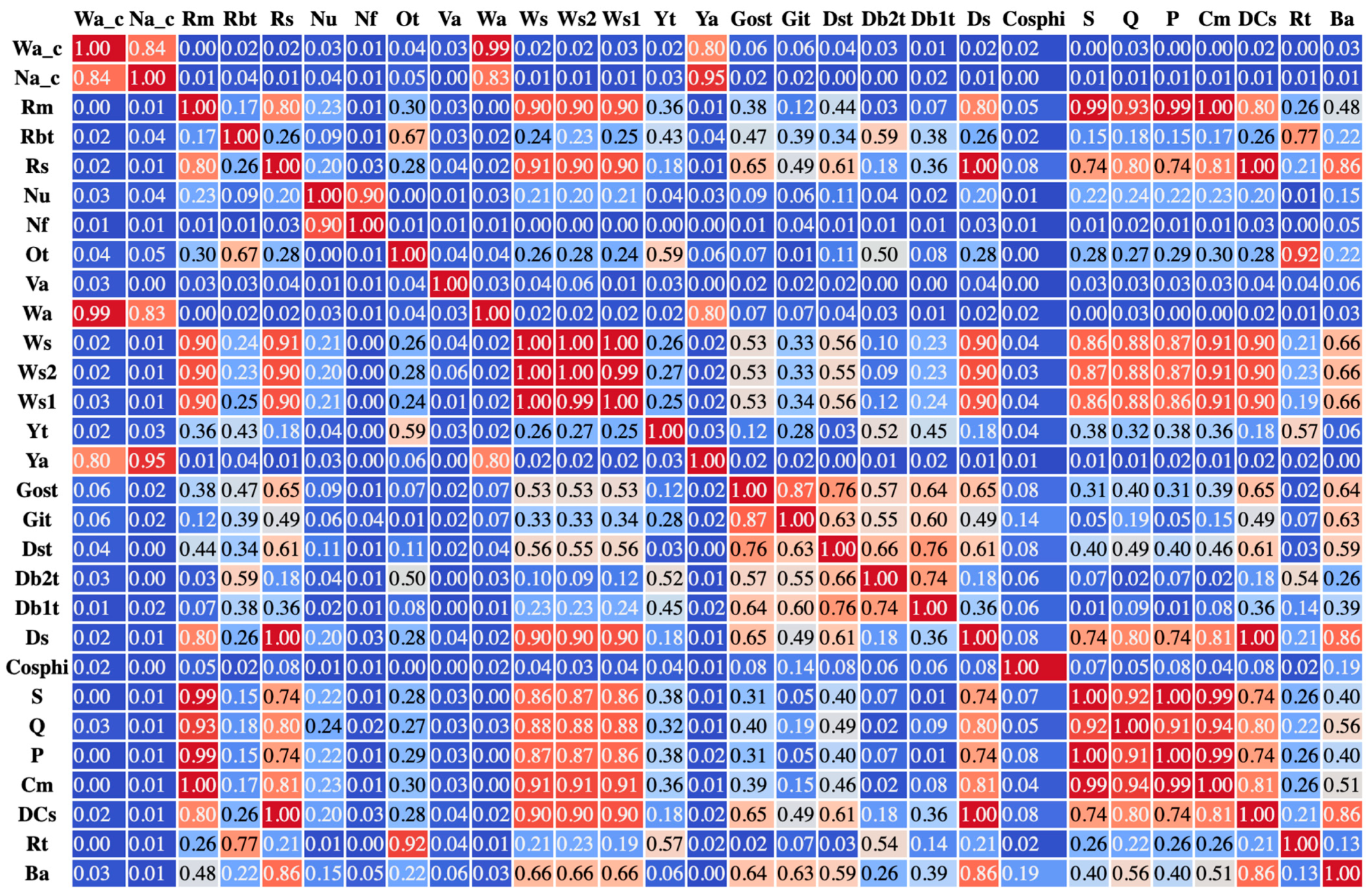
The second step (i.e., dimensionality reduction) was conducted by performing the Pearson correlation coefficient analysis. This helps to improve the training process since linearly dependent variables do not contribute much to the final outcome, and they only increase the dimensionality of the problem, thus making it harder to properly tune models. The process was conducted by iterating over each input variable and comparing its correlation coefficient against every other feature. If the absolute value is greater than or equal to a threshold, then that variable is added to a set of columns to be dropped, provided the other feature is not present there already. This allows us to keep the most informative variables. Eventually, for the absolute value of the correlation coefficient equal to 0.75, the number of input features was reduced down to the following 12: corrected absolute wind direction, torque, rotor bearing temperature, grid voltage, outdoor temperature, vane position, nacelle temperature, gearbox oil sump temperature, both measurements of generator bearing temperature, power factor (ratio of active to apparent power), and pitch angle. The correlation matrix for all initially considered input variables is shown in Figure 3. A summary of the selected input features and their physical units is given in Table 1.
The last step (i.e., data scaling) is the min-max data standardisation, which allows us to bring all features into the common range [0, 1]. Therefore, it can help to increase models’ prediction power as all features are equally important for algorithms—particularly in the case of neural networks.
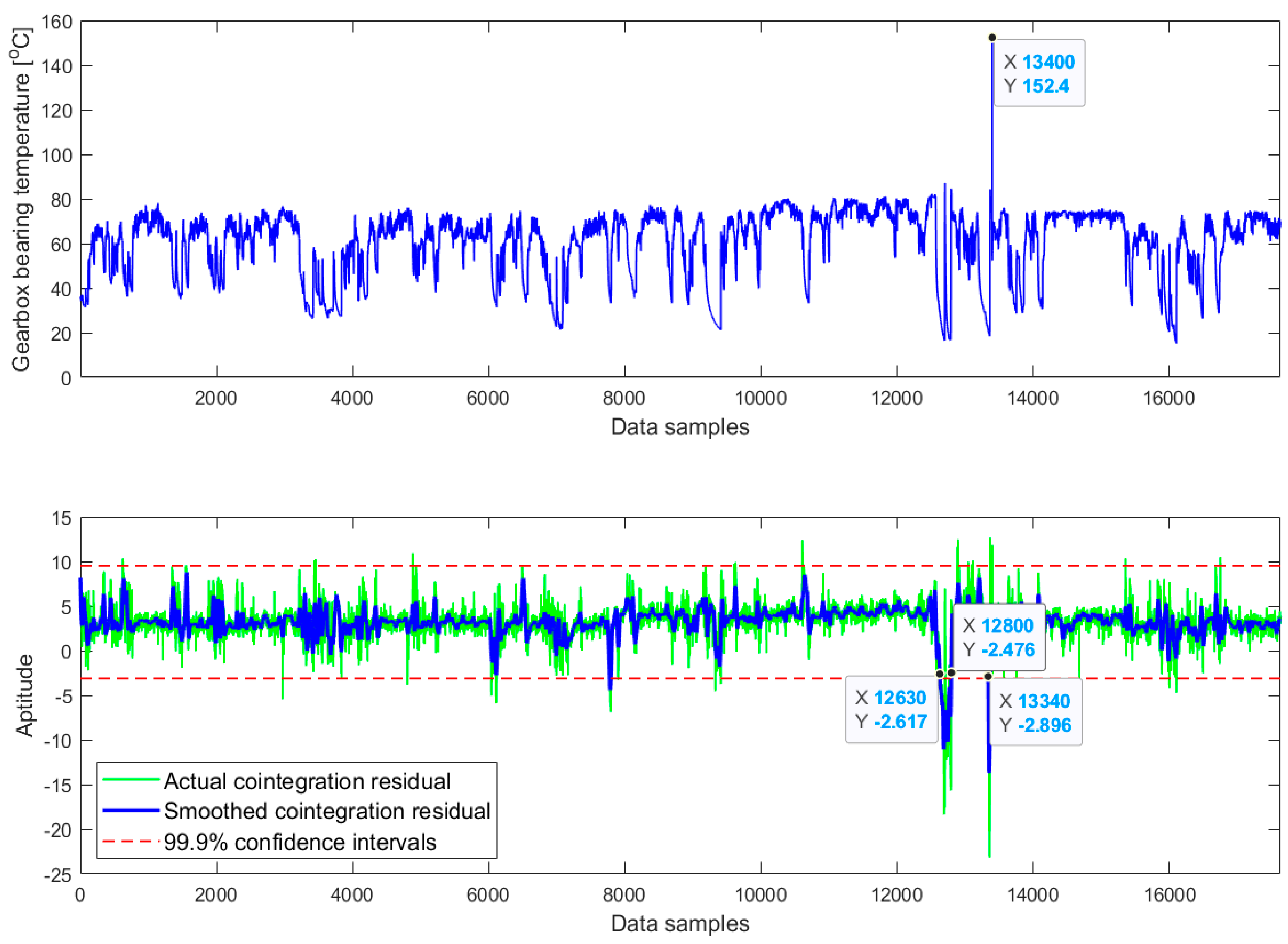
As shown in Figure 1, the apparent gearbox fault, which is physically indicated by an abnormal temperature peak (152 °C), occurred on 2 January 2015 at 13:50. However, it may be inferred that the fault might have started to develop earlier than this moment. In other words, the degradation of the gearbox subsystem might have gradually progressed over time before developing into the critical failure state on 2 January 2015. Hence, it is important to predict or detect this abnormal behaviour in the turbine gearbox as early as possible. In the following, two solutions using ML algorithms and a cointegration-based approach for early prediction of the turbine gearbox fault are presented and discussed.

4. Condition Monitoring and Fault Detection Using ML Methods

4.1. Training ML-Based Normal Behaviour Models of the Gearbox Bearing Temperature

Four ML models (i.e., LR, MLP, RF, and GBT) were built in this study using the sklearn library [67]. All models have the same output (or target), that is, the gearbox bearing temperature. They are compared altogether based on their performance metrics, including R2 score, MSE, MAE, and maximum error of prediction. Concerning the data division, the first 85% of the preprocessed data (from selected time periods) was used for training (in all cases), while the remaining part was used for testing. The data used for both training and testing were preprocessed by all three steps, as explained in Section 3.2.
The LR model was implemented using the LinearRegression class from the sklearn library. The OLS algorithm was used to estimate the coefficients. The chosen ANN for the study was the MLP. The network was created using the MLPRegressor class from the sklearn library. An appropriate topology of the network, including the number of hidden layers and neurons at each layer, was selected during the tuning process. The resulting network consisted of two hidden layers, both with 50 nodes. The remaining parameters of the MLP model were chosen as follows: the solver was ADAMs, which is a stochastic gradient-based optimiser working well on large datasets; the initial learning rate was equal to 0.05, which is responsible for step-size in updating weights; and the rectified linear unit function was selected as an activation function because output values are real positive numbers.
The RF model was formed using the RandomForestRegressor class from the sklearn library. A commonly used criterion to obtain high-performance scores of the algorithm is to minimise the MSE. The number of trees in the forest was, by default, set to 100 because, for the employment of a larger forest, there was not any significant improvement in the results. The XGBoost implementation of the GBT was chosen in this study because it provides support for GPU-accelerated training and is highly flexible and scalable. Eventually, the best-obtained configuration includes 100 estimators with a maximum depth of 6 for a learning rate equal to 0.1.
The best set of hyperparameters for MLP, RF, and XGBoost models was found using the grid search with cross-validation with 4 folds, which tried to maximise the negative MSE and R2 score. In every case, the search space was created by investigating different values for parameters discussed above for each model respectively, which are as follows:
  • MLP: number of hidden layers and neurons within a layer, and learning rate;
  • RF: number of estimators;
  • XGBoost: number of estimators, maximum depth of a tree, and learning rate.
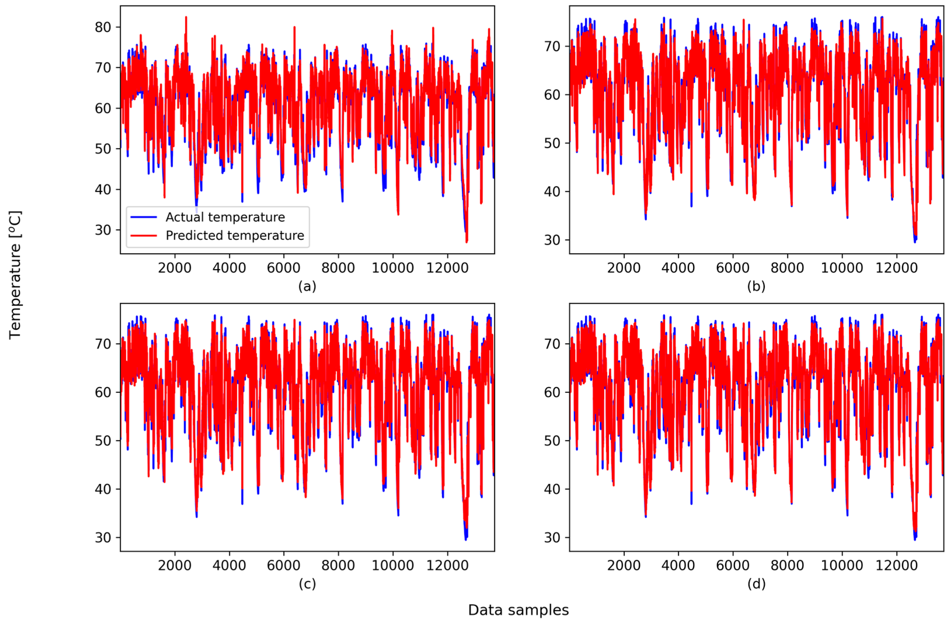
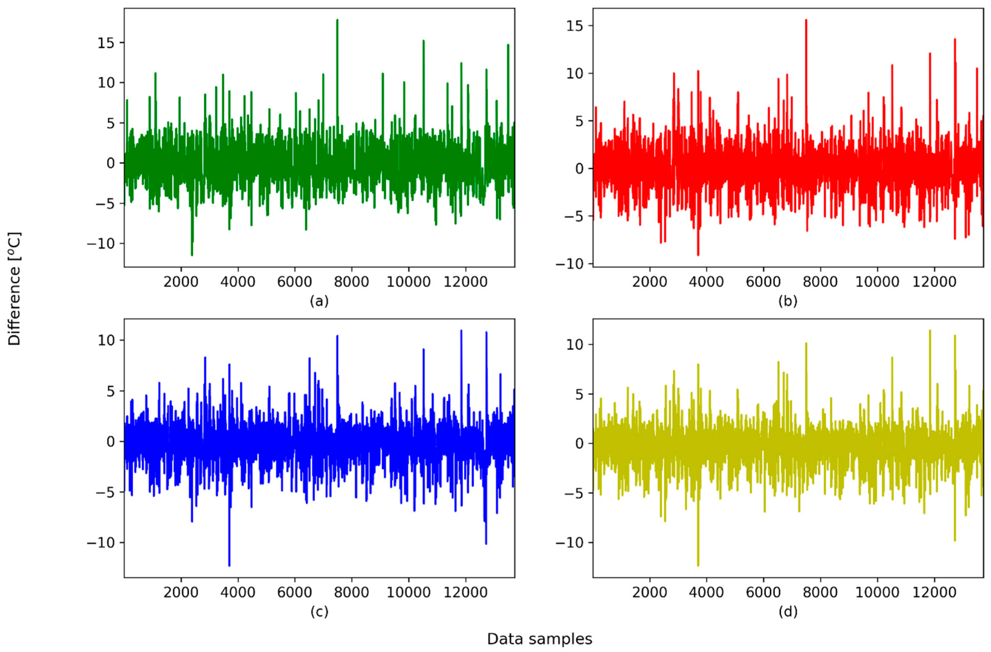
Comparisons of performance metrics obtained for different ML models are shown in Table 2 and Table 3 for the training and testing steps, respectively. In addition, the true and predicted values of the gearbox bearing temperature obtained for the LR mode, MLP model, RF, and XGBoost model are plotted in Figure 4. Figure 5 represents the error analysis for all models on the same predictions. Based on these results, both the RF and the XGBoost models have been chosen as the best ones and used for predicting gearbox failure.

4.2. Testing the XGBoost Model for the Prediction of the Gearbox Failure

The XGBoost model was validated by predicting the gearbox failure occurred on 2 January 2015 at 13:50 (see Figure 1). The testing data spans over four months, from 1 October 2014 to 31 January 2015 (in total, 17,638 samples). The interval begins with a region containing samples representing the wind turbine under healthy operating conditions so as to calculate statistical indexes and to specify a reference for the comparison with the abnormal behaviour of the wind turbine during a failure mode. To designate the occurrence of gearbox faults, an alarm threshold is calculated based on the 99.9% statistical confidence intervals. A confidence interval—with respect to the average of a given time series—is calculated as ν ± 3 σ , where ν and σ are the mean and standard deviation.
Figure 6 plots the actual and predicted values of the gearbox bearing temperature calculated for the test case. Figure 7 depicts a control chart showing a long-term abrupt change in the difference (or residual) between the actual and predicted gearbox bearing temperature. To ease the fault detection process and its interpretation, we employed the Savitzky–Golay filter [68,69] using the moving window with a size of 50 to smooth the difference between the actual and predicted gearbox bearing temperature. The Savitzky–Golay filter, utilising a quadratic polynomial, serves as a smoothing technique that proves more efficient than alternative methods, particularly when dealing with rapidly fluctuating data. It is noted that we interpret and discuss the fault detection process using the smoothed temperature difference and the 99.9% statistical confidence intervals. Figure 7 reveals that the smoothed temperature difference crosses the alarm threshold for the first time at sample 7050 and for the second time at sample 7892. It then remains outside the threshold most of the time until sample 13,400, which corresponds to the peak of the temperature difference (about 110 °C). This is exactly the moment when the gearbox fault reached the critical failure state on 2 January 2015 at 13:50, as displayed in Figure 1.
We could consider setting a warning state (i.e., implying that the wind turbine might have exhibited abnormal behaviour) after the smoothed temperature difference crossed the alarm threshold for the first time at sample 7050. Then, when the abrupt change repeated the second time at sample 7892 (about 140 h after the first time), we could consider it as a critical state alert (i.e., a potential failure in the wind turbine might occur soon). Since sample 13,400 indicates the moment when the actual fault occurred in the turbine gearbox, this implies that the XGBoost-based condition monitoring model would be able to predict the actual fault 918 h (13,400 − 7892 samples) or 38 days before it eventually happened on 2 January 2015 at 13:50.

4.3. Testing the RF Model for the Prediction of the Gearbox Failure

The same 17,638 data samples, recorded between 1 October 2014 and 31 January 2015, previously used to validate the XGBoost model, were used to test the RF model. Figure 8 plots the actual and predicted values of the gearbox bearing temperature calculated for the test case. We can observe from Figure 9 that the smoothed temperature difference crossed the alarm threshold for the first time at sample 6993 and for the second time at sample 7898 (about 150 h between these two events). Generally, the results produced by the RF model are very similar to those obtained from the XGBoost model. In particular, the shapes of the temperature difference in Figure 7 and Figure 9 are very similar to each other. In this case, the RF-based condition monitoring model was able to predict the gearbox failure 917 h (13,400 − 7898 samples) or 38 days before it physically manifested as a temperature peak (152 °C) on 2 January 2015 at 13:50. In summary, we can conclude that both the XGBoost- and RF-based condition monitoring models could predict the actual fault 38 days before its actual occurrence.

4.4. Discussion

It should be mentioned that both the XGBoost and RF models resulted in a false alarm around sample 16,000. In addition, both models used a large amount of SCADA data. As explained in Section 3.2, from a total of 21 months of data (about 90,000 samples), 85% of the samples were used for training and 15% for testing the models. This might raise a concern (challenging) for newly installed wind turbines, which may not have such a large amount of data available for these tasks.

5. Condition Monitoring and Fault Detection Using Cointegration Analysis

5.1. Training the Cointegration-Based Monitoring Model

The same four months of SCADA data (17,638 samples), recorded between 1 October 2014 and 31 January 2015, which were previously used to validate the XGBoost and RF models, were also used for the cointegration analysis. The data preprocessing for the cointegration analysis required only the removal of corrupted data (i.e., the first step). The dimensionality reduction and data scaling steps described in Section 3.2 were not necessary. In addition, as reported in the previous works [42,43,44], the cointegration-based monitoring model does not require as much training data as the ML models. Hence, in this study, we used only the first 6000 samples from this 4-month dataset to train the cointegration-based monitoring model and calculate the normalised cointegrating vectors. It is noted that these 6000 samples correspond to the period when the wind turbine was operating under healthy conditions.
Concerning the choice of wind turbine parameters to build the cointegration-based model, the wind speed and generated power were chosen for the cointegration-based monitoring model because the relationship between these two parameters exhibits the so-called wind turbine power curve, which is important for assessing the performance and health conditions of the wind turbine [70]. Furthermore, as highlighted in [27,29,50], temperature parameters of the generator and gearbox should also be incorporated into the model, as faults or abnormal events related to these components typically develop gradually. Early indications of a gearbox or generator fault may emerge several days or even weeks before the actual failure, often manifested by a rise in the temperature of the gearbox bearings and/or the generator. As a result, five process parameters, including the wind speed ( y 1 t ), generator speed ( y 2 t ), generator bearing temperature ( y 3 t ), gearbox bearing temperature ( y 4 t ), and generated power ( y 5 t ) were selected to create the cointegration-based monitoring model, which has the form:
β T Y t = y 1 t β 2 y 2 t β 3 y 3 t β 4 y 4 t β 5 y 5 t
The cointegration-based monitoring model was trained using 6000 samples, as mentioned above. Then, we calculated the normalised cointegrating vectors using Johansen’s cointegration method [33]. The results were as follows: β 1 = 1 ; β 2 = 2.2507 ; β 3 = 0.0007 ; β 4 = 0.0249 ; and β 5 = 0.2059 . The cointegration residual u t was found as
u t = β T Y t + c = y 1 t β 2 y 2 t β 3 y 3 t β 4 y 4 t β 5 y 5 t + c =
y 1 t + 2.2507 y 2 t 0.0007 y 3 t + 0.0249 y 4 t 0.2059 y 5 t + 0.0077
Equation (6) shows that the cointegration residual is derived by multiplying five data vectors ( y 1 t , ,   y 5 t ), which correspond to the five process parameters, by the normalised cointegrating vector. To carry out the online condition monitoring and fault detection for a wind turbine, SCADA data collected from the turbine during regular operating periods (every 10 min) are used for this multiplication. This approach simplifies the monitoring process, as it reduces to observing the stability of the cointegration residual using a control chart.

5.2. Testing the Cointegration-Based Monitoring Model for the Prediction of the Gearbox Failure

Figure 10 shows the cointegration residual plotted against a control chart. Similar to the XGBoost and RF models, an alarm threshold, calculated based on the 99.9% statistical confidence intervals, was used to designate the occurrence of the gearbox fault. To ease the fault detection process and its interpretation, we also employed the Savitzky–Golay filter [68,69], using a moving window with a size of 50 to smooth the cointegration residual. We can observe from Figure 10 that the cointegration residual crossed the alarm threshold for the first time at sample 12,630 and for the second time at sample 13,340. After the first crossing, the residual returned inside the alarm threshold at sample 12,800. This implies that the cointegration residual stayed beyond the alarm threshold for a period of 170 samples (12,800 − 12,630), or almost 29 h. Since the residual remained outside the threshold for more than one day, we could consider it a critical state alert (i.e., a potential failure in the wind turbine might occur soon). Moreover, because sample 13,400 indicates the moment when the actual fault occurred in the turbine gearbox, this implies that the cointegration-based wind turbine monitoring model would be able to predict the actual fault 128.33 h (13,400–12,630 samples) or almost five and a half days before it eventually happened on 2 January 2015 at 13:50. It is noted that, unlike the XGBoost and RF models, the cointegration-based model did not result in a false alarm around sample 16,000.

6. A Proposal for the Combination of ML and Cointegration for Wind Turbine Monitoring

The results in Section 4 and Section 5 indicated that both the XGBoost and RF models provided a very good prediction of gearbox failure (38 days before its actual occurrence), whereas the cointegration-based model was able to predict the actual fault about five and a half days in advance. Since the failure prediction by the two ML models is very early, meaning they forecast a long transition period from the predicted moment to the actual fault, it can be anticipated that the wind farm operator might be confused and find it difficult to make an appropriate decision about the operation of the wind turbine. If the decision is to shut down the wind turbine immediately (or at least as soon as possible) so that a careful technical inspection and/or overall diagnostics of turbine subsystems can be performed, this downtime might ensure the safety of the wind turbine. However, it would result in considerable economic loss for the asset owner, especially if the inspection and diagnostics do not identify any incipient problems with the turbine components. This situation could certainly occur in practice due to incorrect prediction results made by the ML model. If the decision is to keep the wind turbine in regular operating mode, the wind farm owner would face a high risk because the gearbox could eventually fail, leading to a significant economic loss.
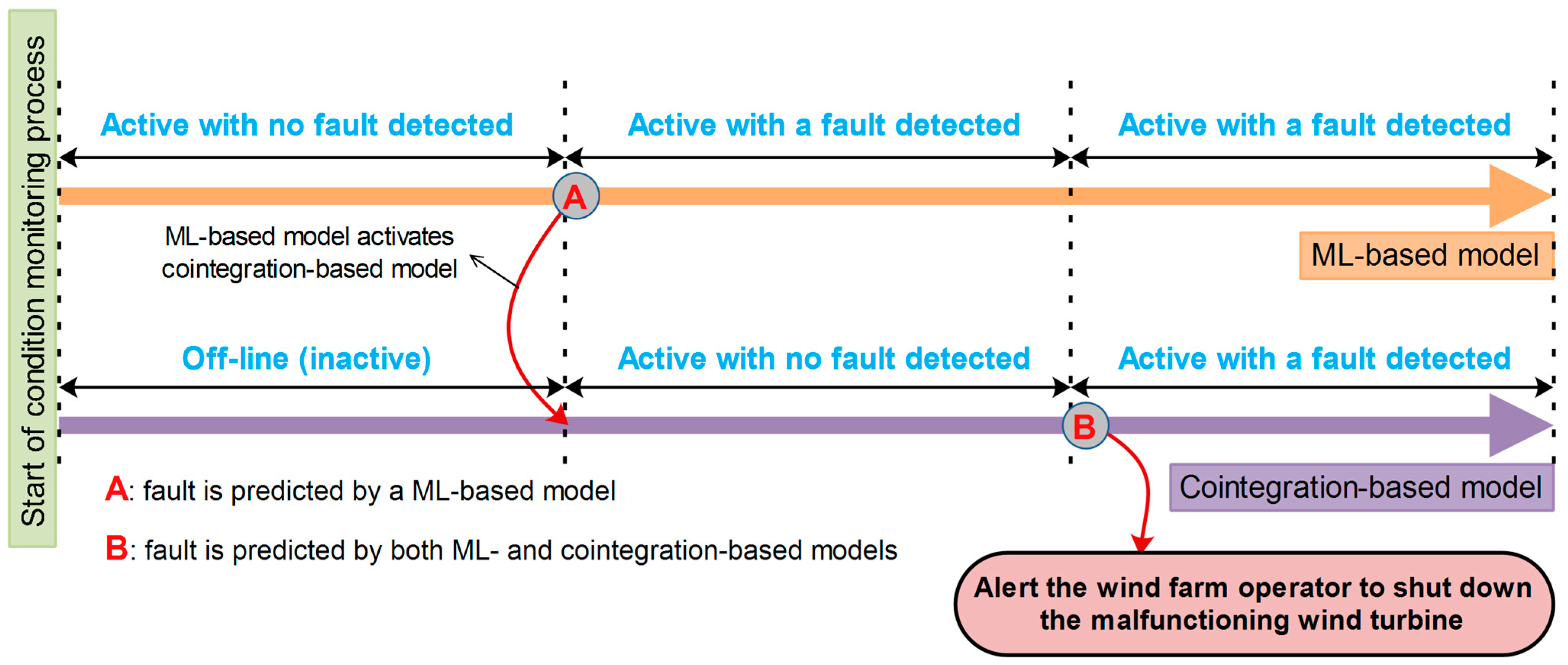
In order to address this trade-off circumstance, a new condition monitoring solution for wind turbines has been proposed in this paper: the ML model (XGBoost or RF) will be implemented in a cascade structure with the cointegration-based model. The former model functions as the outer monitoring process since it provides a long-term prediction, while the latter acts as the inner monitoring process because of its short-term prediction, as depicted in Figure 11. Within this combined scheme, after a fault or failure is predicted early by the ML model, a critical state alert will be sent out, activating the cointegration-based model to monitor the wind turbine in an online manner alongside the ML model. As soon as the cointegration-based model detects a fault or failure, an alarm signal will be sent to the wind farm operator to shut down the malfunctioning wind turbine. In this way, the cointegration-based model is used to validate and confirm the occurrence of the fault or failure previously predicted by the ML model. It is expected that having each wind turbine supervised concurrently by these two data-driven monitoring methods can significantly enhance accuracy and reliability. Additionally, the low computational costs of the cointegration-based approach make it suitable for online (or real-time) monitoring tasks.
Addressing the uncertainties of the models when triggering an alarm is crucial for the practical application of the proposed solution. First, the uncertainties associated with both the ML model and the cointegration-based model, which may stem from factors such as insufficient training data or model bias, can be quantified using probabilistic thresholds. As presented in Section 5, by setting confidence intervals around the gearbox bearing temperature difference and cointegration residual, we can control the false positive and false negative rates. The system will issue early warnings when the predicted anomalies fall outside these intervals, triggering alerts based on predicted probabilities rather than binary outcomes. Second, while the cointegration model’s short-term predictions may delay the detection of some faults, they serve to confirm anomalies flagged by the ML model. By combining both models in a cascade structure, the system reduces the risk of false alarms triggered by uncertainties in the ML model alone. Furthermore, the short-term cointegration-based prediction model helps to pinpoint immediate risks, mitigating the issue of prolonged downtime.
Furthermore, machine downtime and spare part availability are important issues that should be addressed. In practice, once an early warning is issued by the ML model, proactive measures such as initiating spare part procurement and preparing for maintenance can be undertaken before the cointegration-based model confirms the fault. This way, the downtime can be minimised, as maintenance operations can be planned in advance. The early warning provided by the ML model gives operators sufficient time to manage logistics, reducing the impact of prolonged unavailability of spare parts.

7. Conclusions

This paper presents an experimental investigation and comparison between common machine learning algorithms and a cointegration-based approach for condition monitoring and fault detection in wind turbines, using a five-year SCADA dataset from a commercial wind turbine. The comparative analysis focuses on predicting or detecting a gearbox fault at the earliest possible stage. The obtained results confirm that both ML- and cointegration-based approaches can provide early fault detection for wind turbines, allowing for timely maintenance and reduced downtime. Compared to the XGBoost and RF models, the cointegration-based monitoring solution did not offer very early predictions of the gearbox fault. However, the advantages of the cointegration-based approach are its simplicity, minimal training data requirements, and low computational costs, which are crucial for practical implementation.
It is argued that, on the one hand, very early fault prediction is important; however, on the other hand, it might make it difficult for the wind farm operator to make a proper (or reasonable) decision about the operation of the wind turbine, such as whether to shut it down or keep it operating under possible risks. Taking into account the strengths of both approaches, we propose combining ML and cointegration in a cascade monitoring structure. The ML model serves as the outer monitoring process, providing long-term predictions, while the cointegration-based model functions as the inner monitoring process, offering short-term predictions. Supervising each wind turbine concurrently with these two data-driven monitoring methods can significantly enhance accuracy and reliability. Therefore, the deployment of this combined approach is expected to improve the safety, reliability, and operating performance of wind turbines. The proposed solution combines the strengths of both models and handles uncertainties using probabilistic thresholds. This strategy minimises downtime and allows for more efficient planning and resource allocation during the maintenance process.
The future work will focus on several key areas to enhance and extend the proposed condition monitoring solution. First, it is important to validate the proposed approach using SCADA datasets from various wind turbines under different environmental and load conditions that include a wider range of fault types affecting various turbine components. Second, it is necessary to investigate the use of other machine learning models and hybrid approaches, such as combining deep learning with the current cascade structure, to enhance early fault detection. This would include testing different architectures like recurrent neural networks or transformer models to capture more complex temporal patterns in the data.

Author Contributions

Conceptualisation, P.K. and P.B.D.; methodology, P.K. and P.B.D.; software, P.K. and P.B.D.; validation, P.K. and P.B.D.; formal analysis, P.K. and P.B.D.; investigation, P.K. and P.B.D.; resources, P.K. and P.B.D.; data curation, P.K. and P.B.D.; writing—original draft preparation, P.K. and P.B.D.; writing—review and editing, P.K. and P.B.D.; visualisation, P.K. and P.B.D.; supervision, P.B.D.; funding acquisition, P.B.D. All authors have read and agreed to the published version of the manuscript.

Funding

The work presented in this paper was performed within the scope of the research grant No. UMO-2023/51/B/ST8/01253 financed by the National Science Centre (NCN), Poland.

Data Availability Statement

The original contributions presented in the study are included in the article, further inquiries can be directed to the corresponding author.

Acknowledgments

The SCADA data used in this study come from the La Houte Borne wind farm in Villeneuve-d’Ascq, France. The authors would like to thank the ENGIE company for sharing the wind farm datasets for public use.

Conflicts of Interest

Author Paweł Knes was employed by the company IBM Poland. The remaining author declares that the research was conducted in the absence of any commercial or financial relationships that could be construed as a potential conflict of interest.

Nomenclature/Abbreviation

ANNArtificial Neural Network
AIArtificial Intelligence
CNNConvolutional Neural Network
DNNDeep Neural Network
DTDecision Tree
GBTGradient Boosting Tree
LRLinear Regression
LSTMLong Short-Term Memory
MAEMean Absolute Error
MLMachine Learning
MLPMultilayer Perceptron
MSEMean-Squared Error
OLSOrdinary Least Squares
O&MOperation and Maintenance
RFRandom Forest
SCADASupervisory Control and Data Acquisition
SVMSupport Vector Machine

References

  1. Global Wind Energy Council. Global Wind Report: Annual Market Update 2024. Available online: https://gwec.net/global-wind-report-2024/ (accessed on 16 April 2024).
  2. Gao, Z.; Liu, X. An overview on fault diagnosis, prognosis and resilient control for wind turbine systems. Processes 2021, 9, 300. [Google Scholar] [CrossRef]
  3. Khan, P.W.; Byun, Y.C. A review of machine learning techniques for wind turbine’s fault detection, diagnosis, and prognosis. Int. J. Green Energy 2024, 21, 771–786. [Google Scholar] [CrossRef]
  4. Murgia, A.; Verbeke, R.; Tsiporkova, E.; Terzi, L.; Astolfi, D. Discussion on the suitability of SCADA-based condition monitoring for wind turbine fault diagnosis through temperature data analysis. Energies 2023, 16, 620. [Google Scholar] [CrossRef]
  5. Morrison, R.; Liu, X.; Lin, Z. Anomaly detection in wind turbine SCADA data for power curve cleaning. Renew. Energy 2022, 184, 473–486. [Google Scholar] [CrossRef]
  6. Pozo, F.; Vidal, Y.; Salgado, Ó. Wind turbine condition monitoring strategy through multiway PCA and multivariate inference. Energies 2018, 11, 749. [Google Scholar] [CrossRef]
  7. Chen, P.; Lin, Z.; Xie, Z.; Qu, C. Real-time yaw-misalignment calibration and field-test verification of wind turbine via machine learning methods. Mech. Syst. Signal Process. 2024, 208, 110972. [Google Scholar] [CrossRef]
  8. Castellani, F.; Astolfi, D.; Sdringola, P.; Proietti, S.; Terzi, L. Analyzing wind turbine directional behavior: SCADA data mining techniques for efficiency and power assessment. Appl. Energy 2017, 185, 1076–1086. [Google Scholar] [CrossRef]
  9. Stetco, A.; Dinmohammadi, F.; Zhao, X.; Robu, V.; Flynn, D.; Barnes, M.; Keane, J.; Nenadic, G. Machine learning methods for wind turbine condition monitoring: A review. Renew. Energy 2019, 133, 620–635. [Google Scholar] [CrossRef]
  10. Chandrasekhar, K.; Stevanovic, N.; Cross, E.J.; Dervilis, N.; Worden, K. Damage detection in operational wind turbine blades using a new approach based on machine learning. Renew. Energy 2021, 168, 1249–1264. [Google Scholar] [CrossRef]
  11. Santolamazza, A.; Dadi, D.; Introna, V. A data-mining approach for wind turbine fault detection based on SCADA data analysis using artificial neural networks. Energies 2021, 14, 1845. [Google Scholar] [CrossRef]
  12. Bangalore, P.; Letzgus, S.; Karlsson, D.; Patriksson, M. An artificial neural network-based condition monitoring method for wind turbines, with application to the monitoring of the gearbox. Wind Energy 2017, 20, 1421–1438. [Google Scholar] [CrossRef]
  13. Cui, Y.; Bangalore, P.; Tjernberg, L.B. A fault detection framework using recurrent neural networks for condition monitoring of wind turbines. Wind Energy 2021, 24, 1249–1262. [Google Scholar] [CrossRef]
  14. Xiang, L.; Wang, P.; Yang, X.; Hu, A.; Su, H. Fault detection of wind turbine based on SCADA data analysis using CNN and LSTM with attention mechanism. Measurement 2021, 175, 109094. [Google Scholar] [CrossRef]
  15. Ulmer, M.; Jarlskog, E.; Pizza, G.; Manninen, J.; Goren Huber, L. Early fault detection based on wind turbine SCADA data using convolutional neural networks. PHM Soc. Eur. Conf. 2020, 5, 9. [Google Scholar] [CrossRef]
  16. Teng, W.; Cheng, H.; Ding, X.; Liu, Y.; Ma, Z.; Mu, H. DNN-based approach for fault detection in a direct drive wind turbine. IET Renew. Power Gener. 2018, 12, 1164–1171. [Google Scholar] [CrossRef]
  17. Zhao, H.; Liu, H.; Hu, W.; Yan, X. Anomaly detection and fault analysis of wind turbine components based on deep learning network. Renew. Energy 2018, 127, 825–834. [Google Scholar] [CrossRef]
  18. Sun, S.; Wang, T.; Yang, H.; Chu, F. Condition monitoring of wind turbine blades based on self-supervised health representation learning: A conducive technique to effective and reliable utilization of wind energy. Appl. Energy 2022, 313, 118882. [Google Scholar] [CrossRef]
  19. Ren, H.; Liu, W.; Shan, M.; Wang, X. A new wind turbine health condition monitoring method based on VMD-MPE and feature-based transfer learning. Measurement 2019, 148, 106906. [Google Scholar] [CrossRef]
  20. Zhan, J.; Wu, C.; Ma, X.; Yang, C.; Miao, Q.; Wang, S. Abnormal vibration detection of wind turbine based on temporal convolution network and multivariate coefficient of variation. Mech. Syst. Signal Process. 2022, 174, 109082. [Google Scholar] [CrossRef]
  21. Zhang, K.; Tang, B.; Deng, L.; Liu, X. A hybrid attention improved ResNet based fault diagnosis method of wind turbines gearbox. Measurement 2021, 179, 109491. [Google Scholar] [CrossRef]
  22. Zhang, Y.; Liu, W.; Wang, X.; Shaheer, M.A. A novel hierarchical hyper-parameter search algorithm based on greedy strategy for wind turbine fault diagnosis. Expert Syst. Appl. 2022, 202, 117473. [Google Scholar] [CrossRef]
  23. Perez-Sanjines, F.; Peeters, C.; Verstraeten, T.; Antoni, J.; Nowé, A.; Helsen, J. Fleet-based early fault detection of wind turbine gearboxes using physics-informed deep learning based on cyclic spectral coherence. Mech. Syst. Signal Process. 2023, 185, 109760. [Google Scholar] [CrossRef]
  24. Qiao, L.; Zhang, Y.; Wang, Q. Fault detection in wind turbine generators using a meta-learning-based convolutional neural network. Mech. Syst. Signal Process. 2023, 200, 110528. [Google Scholar] [CrossRef]
  25. Yang, X.; Zhang, Y.; Wu, X.; Liu, G. Failure mode classification of IGBT modules under power cycling tests based on data-driven machine learning framework. IEEE Trans. Power Electron. 2023, 38, 16130–16141. [Google Scholar] [CrossRef]
  26. Ma, G.; Xu, S.; Jiang, B.; Cheng, C.; Yang, X.; Shen, Y.; Yang, T.; Huang, Y.; Ding, H.; Yuan, Y. Real-time personalized health status prediction of lithium-ion batteries using deep transfer learning. Energy Environ. Sci. 2022, 15, 4083–4094. [Google Scholar] [CrossRef]
  27. Attia, P.M.; Grover, A.; Jin, N.; Severson, K.A.; Markov, T.M.; Liao, Y.H.; Chen, M.H.; Cheong, B.; Perkins, N.; Yang, Z.; et al. Closed-loop optimization of fast-charging protocols for batteries with machine learning. Nature 2020, 578, 397–402. [Google Scholar] [CrossRef]
  28. Yampikulsakul, N.; Byon, E.; Huang, S.; Sheng, S.; You, M. Condition monitoring of wind power system with nonparametric regression analysis. IEEE Trans. Energy Convers. 2014, 29, 288–299. [Google Scholar]
  29. Letzgus, S. Change-point detection in wind turbine SCADA data for robust condition monitoring with normal behaviour models. Wind Energy Sci. 2020, 5, 1375–1397. [Google Scholar] [CrossRef]
  30. Dao, P.B. Condition monitoring and fault diagnosis of wind turbines based on structural break detection in SCADA data. Renew. Energy 2022, 185, 641–654. [Google Scholar] [CrossRef]
  31. Bilendo, F.; Lu, N.; Badihi, H.; Meyer, A.; Cali, Ü.; Cambron, P. Multitarget normal behavior model based on heterogeneous stacked regressions and change-point detection for wind turbine condition monitoring. IEEE Trans. Ind. Inform. 2024, 20, 5171–5181. [Google Scholar] [CrossRef]
  32. Dao, P.B. A CUSUM-based approach for condition monitoring and fault diagnosis of wind turbines. Energies 2021, 14, 3236. [Google Scholar] [CrossRef]
  33. Latiffianti, E.; Sheng, S.; Ding, Y. Wind turbine gearbox failure detection through cumulative sum of multivariate time series data. Front. Energy Res. 2022, 10, 904622. [Google Scholar] [CrossRef]
  34. Dao, P.B. On Wilcoxon rank sum test for condition monitoring and fault detection of wind turbines. Appl. Energy 2022, 318, 119209. [Google Scholar] [CrossRef]
  35. Engle, R.F.; Granger, C.W.J. Cointegration and error-correction: Representation, estimation and testing. Econometrica 1987, 55, 251–276. [Google Scholar] [CrossRef]
  36. Johansen, S. Statistical analysis of cointegration vectors. J. Econ. Dyn. Control 1988, 12, 231–254. [Google Scholar] [CrossRef]
  37. Cross, E.J.; Worden, K.; Chen, Q. Cointegration: A novel approach for the removal of environmental trends in structural health monitoring data. Proc. R. Soc. A 2011, 467, 2712–2732. [Google Scholar] [CrossRef]
  38. Dao, P.B.; Staszewski, W.J. Cointegration approach for temperature effect compensation in Lamb wave based damage detection. Smart Mater. Struct. 2013, 22, 095002. [Google Scholar] [CrossRef]
  39. Tabrizi, A.A.; Al-Bugharbee, H.; Trendafilova, I.; Garibaldi, L. A cointegration-based monitoring method for rolling bearings working in time-varying operational conditions. Meccanica 2017, 52, 1201–1217. [Google Scholar] [CrossRef]
  40. Salvetti, M.; Sbarufatti, C.; Cross, E.J.; Corbetta, M.; Worden, K.; Giglio, M. On the performance of a cointegration-based approach for novelty detection in realistic fatigue crack growth scenarios. Mech. Syst. Signal Process. 2019, 123, 84–101. [Google Scholar] [CrossRef]
  41. He, H.; Wang, W.; Zhang, X. Frequency modification of continuous beam bridge based on co-integration analysis considering the effect of temperature and humidity. Struct. Health Monit. 2019, 18, 376–389. [Google Scholar] [CrossRef]
  42. Tomé, E.S.; Pimentel, M.; Figueiras, J. Damage detection under environmental and operational effects using cointegration analysis—Application to experimental data from a cable-stayed bridge. Mech. Syst. Signal Process. 2020, 135, 106386. [Google Scholar] [CrossRef]
  43. Turrisi, S.; Cigada, A.; Zappa, E. A cointegration-based approach for automatic anomalies detection in large-scale structures. Mech. Syst. Signal Process. 2022, 166, 108483. [Google Scholar] [CrossRef]
  44. Dao, P.B.; Staszewski, W.J. Cointegration and how it works for structural health monitoring. Measurement 2023, 209, 112503. [Google Scholar] [CrossRef]
  45. Dao, P.B.; Staszewski, W.J.; Barszcz, T.; Uhl, T. Condition monitoring and fault detection in wind turbines based on cointegration analysis of SCADA data. Renew. Energy 2018, 116, 107–122. [Google Scholar] [CrossRef]
  46. Dao, P.B.; Staszewski, W.J.; Uhl, T. Operational condition monitoring of wind turbines using cointegration method. In Advances in Condition Monitoring of Machinery in Non-Stationary Operations, Applied Condition Monitoring; Timofiejczuk, A., Chaari, F., Zimroz, R., Bartelmus, W., Haddar, M., Eds.; Chapter 21; Springer: Cham, Switzerland, 2018; Volume 9, pp. 223–233. [Google Scholar]
  47. Dao, P.B. Condition monitoring of wind turbines based on cointegration analysis of gearbox and generator temperature data. Diagnostyka 2018, 19, 63–71. [Google Scholar] [CrossRef]
  48. Sun, X.; Xue, D.; Li, R.; Li, X.; Cui, L.; Zhang, X.; Wu, W. Research on condition monitoring of key components in wind turbine based on cointegration analysis. IOP Conf. Ser. Mater. Sci. Eng. 2019, 575, 012015. [Google Scholar] [CrossRef]
  49. Zhang, B.; Zhang, C.; Duan, H.; Ma, Y.; Li, J.; Cui, L. Realization of condition monitoring of gear box of wind turbine based on cointegration analysis. In Advances in Asset Management and Condition Monitoring; Smart Innovation, Systems and Technologies; Ball, A., Gelman, L., Rao, B., Eds.; Springer: Cham, Switzerland, 2020; Volume 166, pp. 281–291. [Google Scholar]
  50. Zhang, C.; Zhao, G.; Wu, Y. Wind turbine condition monitoring based on SCADA data co-integration analysis. In Mechanisms and Machine Science, Proceedings of the IncoME-VI and TEPEN 2021, Tianjin, China, 20–23 October 2021; Zhang, H., Feng, G., Wang, H., Gu, F., Sinha, J.K., Eds.; Springer: Cham, Switzerland, 2023; Volume 117, pp. 97–103. [Google Scholar]
  51. Qadri, B.A.; Ulriksen, M.D.; Damkilde, L.; Tcherniak, D. Cointegration for detecting structural blade damage in an operating wind turbine: An experimental study. In Dynamics of Civil Structures, Proceedings of the 37th IMAC, A Conference and Exposition on Structural Dynamics 2019, Orlando, FL, USA, 28–31 January 2019; Pakzad, S., Ed.; Conference Proceedings of the Society for Experimental Mechanics Series; Springer: Cham, Switzerland, 2020; Volume 2, pp. 173–180. [Google Scholar]
  52. Xu, M.; Li, J.; Wang, S.; Yang, N.; Hao, H. Damage detection of wind turbine blades by Bayesian multivariate cointegration. Ocean Eng. 2022, 258, 111603. [Google Scholar] [CrossRef]
  53. Dao, P.B. On cointegration analysis for condition monitoring and fault detection of wind turbines using SCADA data. Energies 2023, 16, 2352. [Google Scholar] [CrossRef]
  54. Wu, Z.; Li, Y.; Wang, P. A hierarchical modeling strategy for condition monitoring and fault diagnosis of wind turbine using SCADA data. Measurement 2024, 227, 114325. [Google Scholar] [CrossRef]
  55. Kuai, H.; Civera, M.; Coletta, G.; Chiaia, B.; Surace, C. Cointegration strategy for damage assessment of offshore platforms subject to wind and wave forces. Ocean Eng. 2024, 304, 117692. [Google Scholar] [CrossRef]
  56. Zolna, K.; Dao, P.B.; Staszewski, W.J.; Barszcz, T. Nonlinear cointegration approach for condition monitoring of wind turbines. Math. Probl. Eng. 2015, 2015, 978156. [Google Scholar] [CrossRef]
  57. Salameh, J.P.; Cauet, S.; Etien, E.; Sakout, A.; Rambault, L. Gearbox condition monitoring in wind turbines: A review. Mech. Syst. Signal Process. 2018, 111, 251–264. [Google Scholar] [CrossRef]
  58. Artigao, E.; Martín-Martínez, S.; Honrubia-Escribano, A.; Gómez-Lázaro, E. Wind turbine reliability: A comprehensive review towards effective condition monitoring development. Appl. Energy 2018, 228, 1569–1583. [Google Scholar] [CrossRef]
  59. Jin, X.; Xu, Z.; Qiao, W. Condition monitoring of wind turbine generators using SCADA data analysis. IEEE Trans. Sustain. Energy 2021, 12, 202–210. [Google Scholar] [CrossRef]
  60. Meyer, A. Multi-target normal behaviour models for wind farm condition monitoring. Appl. Energy 2021, 300, 117342. [Google Scholar] [CrossRef]
  61. Castellani, F.; Natili, F.; Astolfi, D.; Vidal, Y. Wind turbine gearbox condition monitoring through the sequential analysis of industrial SCADA and vibration data. Energy Rep. 2024, 12, 750–761. [Google Scholar] [CrossRef]
  62. Dao, P.B.; Barszcz, T.; Staszewski, W.J. Anomaly detection of wind turbines based on stationarity analysis of SCADA data. Renew. Energy 2024, 232, 121076. [Google Scholar] [CrossRef]
  63. Géron, A. Hands-On Machine Learning with Scikit-Learn and TensorFlow: Concepts, Tools, and Techniques to Build Intelligent Systems, 1st ed.; O’Reilly Media, Inc.: Sebastopol, CA, USA, 2017; 572p. [Google Scholar]
  64. Zivot, E.; Wang, J. Modeling Financial Time Series with S-PLUS, 2nd ed.; Springer: New York, NY, USA, 2006. [Google Scholar]
  65. LeSage, J.P. Econometrics Toolbox. Available online: https://www.spatial-econometrics.com (accessed on 27 August 2024).
  66. ENGIE OpenData. SCADA Datasets of La Houte Bourne Wind Farm. Available online: https://opendata-renewables.engie.com/explore/index (accessed on 18 September 2023).
  67. Scikit-Learn. Machine Learning in Python. Available online: https://scikit-learn.org/stable/ (accessed on 16 May 2024).
  68. Savitzky, A.; Golay, M.J.E. Smoothing and differentiation of data by simplified least squares procedures. Anal. Chem. 1964, 36, 1627–1639. [Google Scholar] [CrossRef]
  69. Luo, J.; Ying, K.; Bai, J. Savitzky–Golay smoothing and differentiation filter for even number data. Signal Process. 2005, 85, 1429–1434. [Google Scholar] [CrossRef]
  70. Bilendo, F.; Meyer, A.; Badihi, H.; Lu, N.; Cambron, P.; Jiang, B. Applications and modeling techniques of wind turbine power curve for wind farms—A review. Energies 2023, 16, 180. [Google Scholar] [CrossRef]
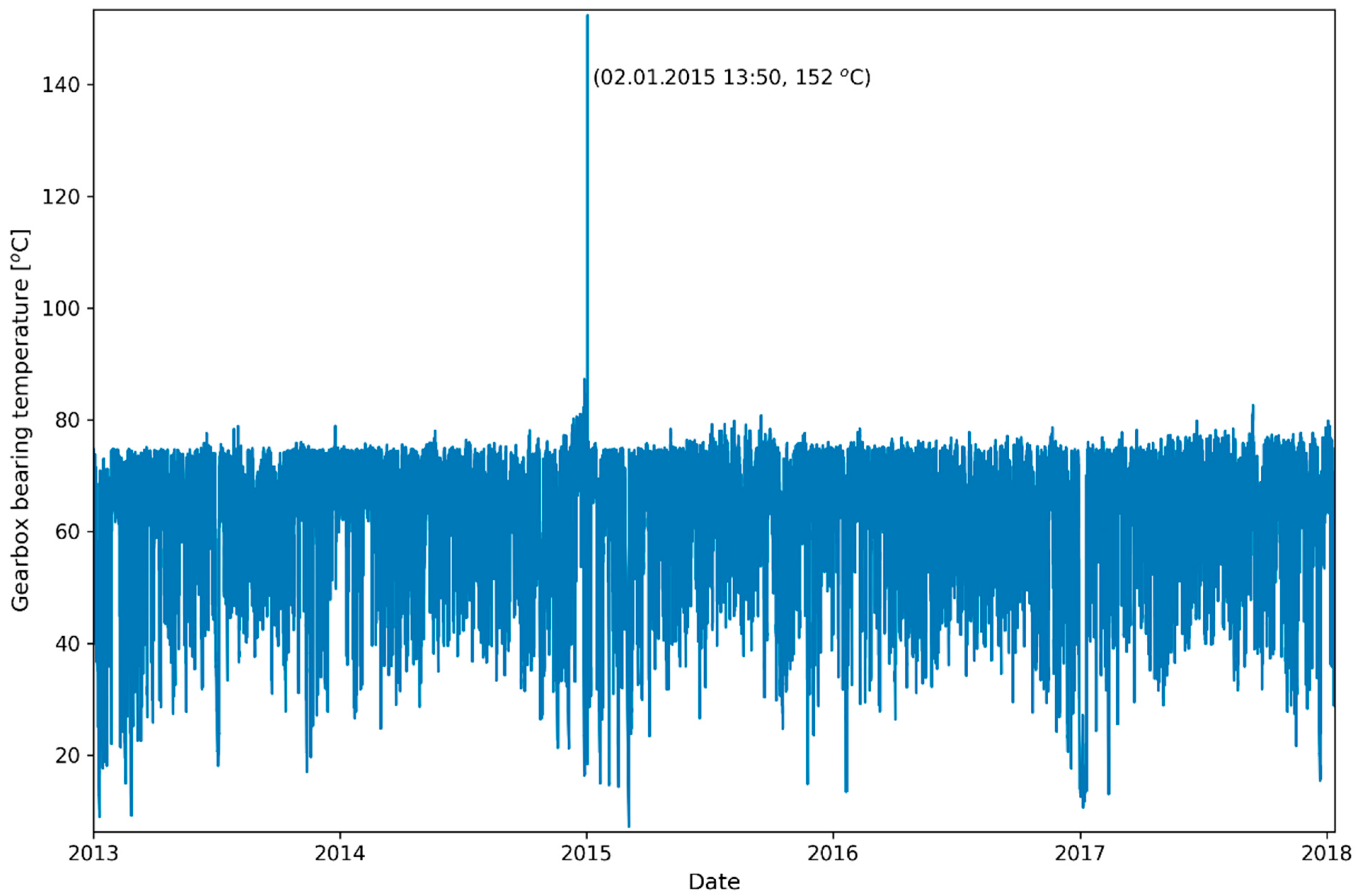
Figure 1. Gearbox bearing temperature over 5 years of measurements, showing a gearbox fault exhibited by an abnormal temperature peak (152 °C) that occurred on 2 January 2015 at 13:50.
Energies 17 05055 g001
Figure 2. Histogram of gearbox bearing temperature values with the selected ranges marked by red vertical lines.
Energies 17 05055 g002
Figure 3. Pearson correlation matrix (absolute values) for all investigated input variables.
Energies 17 05055 g003
Figure 4. Comparison of true and predicted values of the gearbox bearing temperature for all trained models on test samples: (a) LR, (b) MLP, (c) RF, and (d) XGB.
Energies 17 05055 g004
Figure 5. Comparison of differences between true and predicted values of the gearbox bearing temperature for all trained models on test samples: (a) LR, (b) MLP, (c) RF, and (d) XGB.
Energies 17 05055 g005
Figure 6. Actual and predicted values of the gearbox bearing temperature obtained for the test case using the XGBoost model: (top) the entire test case interval and (bottom) part of the interval where both graphs start to diverge significantly.
Energies 17 05055 g006
Figure 7. Control chart showing a long-term abrupt change in the difference between the actual and predicted gearbox bearing temperature (XGBoost model).
Energies 17 05055 g007
Figure 8. Actual and predicted values of the gearbox bearing temperature obtained for the test case using the RF model: (top) the entire test case interval and (bottom) part of the interval where both graphs start to diverge significantly.
Energies 17 05055 g008
Figure 9. Control chart showing a long-term abrupt change in the difference between the actual and predicted gearbox bearing temperature (RF model).
Energies 17 05055 g009
Figure 10. Gearbox failure detection using cointegration: (top) gearbox bearing temperature and (bottom) control chart showing an abrupt change in the cointegration residual.
Energies 17 05055 g010
Figure 11. A combined scheme of ML and cointegration for wind turbine condition monitoring: The ML model functions as the outer process (long-term prediction), while the cointegration model acts as the inner process (short-term prediction).
Energies 17 05055 g011
Table 1. Input parameters of the model.
No.ParametersAbbreviationUnitsPearson Corr. Coefficient (min–max)
1Absolute wind direction correctedWa_cdeg0.00–0.99
2TorqueRmNm0.00–1.00
3Rotor bearing temperatureRbt°C0.00–0.77
4Grid voltageNuV0.00–0.90
5Outdoor temperatureOt°C0.00–0.92
6Vane positionVadeg0.00–0.06
7Nacelle temperatureYt°C0.00–0.59
8Gearbox oil sump temperatureGost°C0.01–0.87
9Generator bearing temperature 1Db1t°C0.00–0.76
10Generator bearing temperature 2Db2t°C0.00–0.74
11Power factorCosphi[-]0.00–0.19
12Pitch angleBadeg0.00–0.86
Table 2. Comparison of performance metrics obtained for four ML methods (training step).
MethodTraining TimeR2 ScoreMSEMAEMax. Error
LR0.058 [s]0.9534.4021.47822.194
MLP7.431 [s]0.9732.5661.10519.998
RF96.585 [s]0.9980.2060.3026.923
XGBoost0.302 [s]0.9861.3330.81910.690
Table 3. Comparison of performance metrics obtained for four ML methods (testing step).
MethodInference TimeR2 ScoreMSEMAEMax. Error
LR0.001 [s]0.9543.8661.41717.771
MLP0.010 [s]0.9712.4471.09415.578
RF0.303 [s]0.9752.1341.03012.358
XGBoost0.007 [s]0.9771.9780.99112.376
Disclaimer/Publisher’s Note: The statements, opinions and data contained in all publications are solely those of the individual author(s) and contributor(s) and not of MDPI and/or the editor(s). MDPI and/or the editor(s) disclaim responsibility for any injury to people or property resulting from any ideas, methods, instructions or products referred to in the content.