Article

Interpretable Wind Power Short-Term Power Prediction Model Using Deep Graph Attention Network

1
School of Electrical Engineering, North China University of Water Resources and Electric Power, Zhengzhou 450045, China
2
School of Mathematics and Statistics, North China University of Water Resources and Electric Power, Zhengzhou 450045, China
3
School of New Energy, North China Electric Power University, Beijing 100096, China
*
Author to whom correspondence should be addressed.
Energies 2024, 17(2), 384; https://doi.org/10.3390/en17020384
Submission received: 28 November 2023 / Revised: 30 December 2023 / Accepted: 9 January 2024 / Published: 12 January 2024
(This article belongs to the Special Issue Control, Real-Time Monitoring and Optimization for Wind Power Systems)

Abstract

:
High-precision spatial-temporal wind power prediction technology is of great significance for ensuring the safe and stable operation of power grids. The development of artificial intelligence technology provides a new scheme for modeling with strong spatial-temporal correlation. In addition, the existing prediction models are mostly ‘black box’ models, lacking interpretability, which may lead to a lack of trust in the model by power grid dispatchers. Therefore, improving the model to obtain interpretability has become an important challenge. In this paper, an interpretable short-term wind power prediction model based on ensemble deep graph neural network is designed. Firstly, the graph network model (GNN) with an attention mechanism is applied to the aggregate and the spatial-temporal features of wind power data are extracted, and the interpretable ability is obtained. Then, the long short-term memory (LSTM) method is used to process the extracted features and establish a wind power prediction model. Finally, the random sampling algorithm is used to optimize the hyperparameters to improve the learning rate and performance of the model. Through multiple comparative experiments and a case analysis, the results show that the proposed model has a higher prediction accuracy than other traditional models and obtains reasonable interpretability in time and space dimensions.

1. Introduction

1.1. Background

With the continuous development of society’s electrification, energy demand has increased rapidly [1]. At the same time, in the context of global warming, countries around the world continue to increase investment in renewable energy to reduce greenhouse gas emissions caused by the use of fossil energy. The use of renewable energy has brought environmental and economic benefits, but the intermittency and variability of renewable energy output power caused by natural conditions have brought challenges to the safe, stable, and reliable operation of the power grid [2]. Wind energy is one of the most widely used renewable energy sources in the world. With the continuous expansion of the scale of wind farms and the continuous optimization of their layout, wind power generation has gradually become the top priority of world energy development [3,4]. Accurate wind power prediction results can make contributions to improving the absorption capacity of the power grid regarding wind power, increasing economic benefits and mitigating climate change [5].

1.2. Related Works

Wind power prediction, as an important part of wind energy consumption, has attracted the attention of a large number of experts and scholars. There are three different types of modelling methods: physical methods, traditional statistical models, and artificial intelligence-based models. Physical methods rely on physical equations [6] and use numerical weather prediction (NWP) data and parameters such as ground roughness, topography [7], and elevation [8] to build prediction models. Statistical methods can directly extrapolate the historical wind power series characteristics to obtain the future wind power. Commonly used statistical methods include the autoregressive model (AR), the autoregressive integrated moving average (ARIMA) model [9], etc. With the rapid development of artificial intelligence and its excellent prediction performance, k-nearest neighbor (KNN), support vector regression (SVR) [10,11,12], deep learning algorithms, etc., have been used in wind power prediction. In recent years, as the computing performance of computers has been greatly improved, deep learning models have attracted the attention of many researchers because of their good generalization performance and ability to deal with high-dimensional data. Commonly used deep models include the convolutional neural network (CNN), recurrent neural network (RNN) [13]. In order to alleviate the limitations of these models, temporal convolutional network (TCN), long short-term memory (LSTM) [14] and gated recurrent unit (GRU) have been derived.
With the advent of the data age, the types of data and the amount of data collected by people through sensors are increasing, which is helpful for researchers to study the laws of related fields more deeply. At present, wind farm data mainly rely on the SCADA system [15] to collect real-time data, and a large number of feature data are obtained with the help of sensors, which is helpful to analyze the running state of the wind turbine. How to use the collected multi-feature data to study the correlation in the deep aspect is a hot topic in wind power prediction research [16,17,18].
Compared with univariate time series modeling, the study found that in order to mine the hidden information of the data at a deeper level, researchers often use the complementary advantages of different models to design an integrated learning method to analyze the correlation information between the original meteorological data and wind power and model prediction. Shan et al. [19] proposed a method to optimize the active power output of DG through artificial neural networks to achieve the elimination of frequency deviation, avoiding the need for direct measurement of the frequency process and adapting to different load changes at the same time. Yildiz et al. [20] used variational mode decomposition (VMD) to extract features and convert them into graphs and then used improved residual-based CNNs for wind power prediction. Wang et al. [21] introduced a real-time prediction method, which used the PSO algorithm to optimize the Markov-based back propagation BP neural network, which improved the model operation speed and produced better prediction results. Zhu et al. [22] used the spatial features extracted by the CNN at the bottom of the model and then captured the time dependence between spatial features through LSTM to form a spatial-temporal prediction model to predict wind speed. Chen et al. [23] proposed a new data reconstruction method based on a three-dimensional matrix and the spatial-temporal prediction method combined with a CNN and LSTM. The proposed model is superior to other baseline models in terms of prediction accuracy and generalization ability. Liu et al. [24] proposed a new spatial-temporal neural network (STNN) to solve the problem of spatial-temporal wind speed prediction by using the image recognition method. The CNN is combined with the gate recurrent unit (GRU) to construct a coding structure to achieve prediction. Although the above prediction models have achieved good prediction results, due to the limitations of the traditional convolution model itself, it cannot adapt to complex data structures, which may lead to information loss [25] and limit the learning ability of the model.
At present, multi-factor features are effective in improving the prediction accuracy of wind power prediction modeling compared with single-factor features. Huang et al. [26] used the Bayesian optimization model to adaptively select the base model by using the coefficient of determination index to tune the hyperparameters, which improved the generalization and prediction accuracy of the prediction model and achieved good prediction results. The spatial-temporal correlation between features in wind power prediction is widespread [27,28]. Using existing methods, although some results have been achieved, the correlation between features is still ignored. Therefore, in order to study the relevant content, some researchers have introduced a method based on a graph neural network to solve this problem. Chen et al. [29] proposed a new spatial-temporal prediction method based on a graph convolutional network (GCN), mining the correlation between features, and the prediction accuracy is better than the baseline model. Zhao et al. [30] combined a GCN with a GRU to capture the spatial-temporal correlation of urban road network traffic. Tao et al. [31] proposed a graph convolutional network based on multi-information spatial-temporal attention (MISTAGCN), which uses the graph convolutional network to mine the potential information of multi-input features and effectively analyzes the spatial-temporal correlation information between different nodes. Based on the analysis of the above literature, it is found that the GCN can learn the correlation information between nodes. At the same time, multi-source information may not be equally important for the success of prediction, and the GAT, composed of the attention mechanism, is used to give nodes different attention. Therefore, using the GAT to extract the temporal and spatial correlation of wind farm historical data will be very helpful for wind power prediction modeling.
Wind turbine power generation is mainly related to the meteorological state at that time [32]. Specifically, wind farm historical data belong to time series, which show temporal features in the horizontal direction and spatial properties between features in the vertical direction. Comprehensive consideration of time and spatial correlation in wind power prediction is very important to improve prediction accuracy. The importance of the time dimension is mainly reflected in long-term, medium-term, and short-term changes. For example, meteorological changes in different seasons and different times of a day are different, resulting in different fluctuation characteristics of wind power generation. This law can be learned through the mining of historical data. The spatial attribute consists of meteorological features through the coupling between them, which is the inherent atmospheric change law of a certain region, and its generation is jointly influenced by the movement of the atmosphere and the terrain environment [33]. At the same time, it can be statistically mined for spatial correlation through a large amount of the historical data [34]. In the process of wind power prediction, the applicability and robustness of the prediction method can be improved by data mining in the time and space dimensions. Recent studies have found that the spatial-temporal correlation between multi-dimensional features is key to accurately predict the output of wind turbines [35,36].
In order to deeply analyze the operation mechanism of the model, this paper will propose an interpretable short-term wind power prediction model based on an integrated deep GNN, which can effectively model the complex meteorological conditions of wind farms. On this basis, the attention mechanism is introduced into the graph network model to express the most relevant variables to wind power, and the time and space dependence between features is deeply explored. At the same time, the interpretability of the model in the time and space dimensions is realized. Finally, multiple cases are used to verify the model proposed in this paper. The prediction process of the spatial-temporal prediction model is shown in Figure 1.

1.3. Research Contributions

Based on the related work and literature research, this paper proposes an interpretable short-term wind power output prediction model based on a graph network model. The main contributions are summarized as follows:
  • Compared with the traditional wind power time series prediction modeling, this paper uses GAT-LSTM as the main method to construct a spatial-temporal prediction model. Firstly, the GAT can extract the information of nodes and edges on the graph and increase the attention of important information between nodes through the attention mechanism and pass the extracted features to the LSTM. Then, the LSTM model performs temporal learning on the extracted features and establishes a prediction model that satisfies the learning target ability.
  • The stochastic search algorithm is applied to the GAT-LSTM prediction model for model hyperparameter optimization, and a multifactor-driven wind power spatial-temporal prediction model is established.
  • Adding attention mechanism to the prediction model, on the one hand, can increase the attention ability of the wind power prediction model to important features and then improve the prediction accuracy of the model. On the other hand, through the dynamic change of the attention weight and the visualization of weight, it can provide a basis for the interpretability of the model more intuitively.

2. Materials and Methods

2.1. Graph Convolution Network

The processing of complex graph data can be achieved through the utilization of a GCN, which draws inspiration from convolutional networks commonly used in computer image recognition [37]. In this field, it is typically necessary to pre-process images into a standardized structure using feature engineering techniques. By leveraging translation invariance within images, convolutional neural networks exhibit excellent feature extraction capabilities [38]. However, real-life graph-structured data often exhibit complexity and irregularity. To enhance the extraction of relevant features, a GCN extends two-dimensional convolutions to the GNN, enabling effective handling of unstructured graph data.
The graph structure is composed of nodes and edges. The graph convolution module uses the connection relationship of edges between nodes to capture the neighbor information of nodes and aggregates this information into each node to perform feature representation on these nodes to deal with the spatial dependence in the graph.
The different node vectors in the GCN are represented by h . The model constructor sets the appropriate number of graph convolution layers N, constructs different node vectors from the input initial features, and constructs the connection between feature nodes through the connection of edges, and the updating of node information is constructed by embedding its own vectors and the information of neighboring nodes, and the new value of the feature at that point obtained by aggregation will be directly passed into the next layer of the features as a propagation object. The new feature value of the point obtained from aggregation will be directly passed into the next layer of features as a propagation object. Here, the GCN calculates the information of each node in the next step at the same time, and the specific settlement process is as follows:
H ( I ) = h 1 ( l ) T , , h N ( l ) T T
H l + 1 = σ D ˜ 1 2 A ˜ D ˜ 1 2 H l W l
By Equation (1), a forward transform is performed for each node feature of the previous layer simultaneously embedded in a matrix. Similarly, the relationship between each node will also form an N × N dimensional adjacency matrix A , A ˜ = A + I is the adjacency matrix of the undirected graph G plus self-connection, so as to aggregate the information of other nodes with their own information. D ˜ is the degree matrix of A ˜ , the element on the diagonal is the degree of each vertex, and the value on the diagonal represents the number of edges associated with the vertex. In Equation (2), the adjacency matrix A ˜ is normalized by D ˜ 1 2 A ˜ D ˜ 1 2 in order to maintain the original distribution of the characteristic matrix H in the process of information transmission and to ensure the stability of model training. W l is the weight vector that needs to be learned in this layer.

2.2. Long Short-Term Memory Neural Network

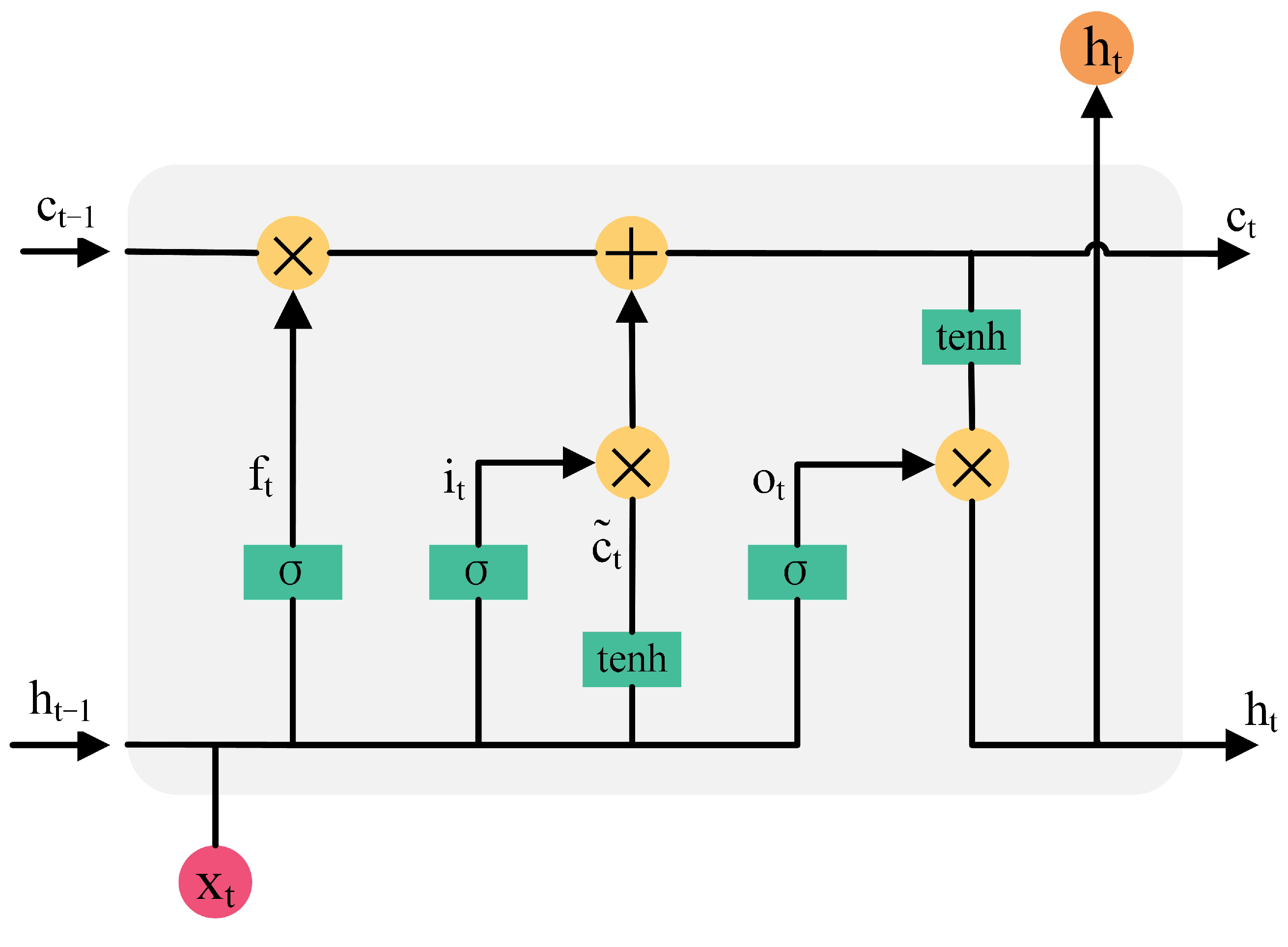
RNNs are often used for deep learning, but the original architecture is prone to gradient disappearance and gradient explosion problems during the learning process of long sequences, resulting in the loss of more important information. As a variant of RNNs, the LSTM can relieve the long-range dependency problem effectively by adding gating mechanism and state units [39]. Figure 2 shows the working flow chart inside the LSTM unit. The LSTM memorizes and transmits important information through the gating mechanism of forgetting, input, and output and forgets some non-important information. The specific calculation procedure is as follows:
f t = sigmoid w f h h t 1 + w f x x t + b f
where w f h and w f x are the weights of the previous output and the current output, respectively, b f is the bias of the forgetting gate, and the nonlinear mapping of sigmoid is performed to determine which unimportant information in the previous output and the new input information is forgotten.
i t = sigmoid w i h h t 1 + w i x x t + b i
c ˜ t = tanh w c h h t 1 + w c x x t + b c
c t = f t c t 1 + i t c ˜ t
Similar to the forgetting gate formula, the main difference is that the sigmoid layer in the input gate determines what is updated, and the tanh layer is used to update the candidate-value state vector c ˜ t , and then to multiply the old state with f t plus the input gate i t and c ˜ t product to obtain the updated cellular c t .
o t = sigmoid w o h h t 1 + w o x x t + b o
h t = o t tanh c t
where w o h and w o x are the weights of the previous output and the current output, respectively, b o is the output gate bias, the sigmoid layer determines the information that contributes to the output, and the cell state is mapped to a value between −1 and 1 after the nonlinear tanh function is processed to control which part of the information needs to be output.

2.3. Graph Attention Mechanism

2.3.1. Attention Mechanism

With the development of sensor technology, engineers have widely used sensors in engineering to record the dynamic changes in the equipment and external environment. For wind turbines, the recorded meteorological feature dimensions are gradually increasing, which is very helpful for the study of wind power generation. However, too many meteorological features unrelated to output can not only improve the prediction accuracy of the model but also cause bad information interference to the model prediction. The attention mechanism is a method that can deeply mine the influence of many features on the output of the wind turbine. In the process of model prediction, different weights are adaptively and dynamically allocated for feature extraction so that the model pays more attention to the feature information with high contribution to the output of the wind turbine, thereby reducing the impact of low or even irrelevant feature information on the prediction model. The introduction of the attention mechanism in this paper can improve the prediction performance of the model. At the same time, the dynamic change trend of the attention coefficient and the final visualization results also provides some basis for the interpretability of the model.

2.3.2. Graph Attention Mechanism

The GCN constructs different nodes in a network structure through the links of edges. When using the Laplacian matrix to obtain node information, there are also problems of high noise, difficult expansion, and high computational cost. Through previous studies, it was found that not all node information is equally important.
In order to improve the learning performance of the graph neural network, the attention mechanism is introduced to form the GAT. The attention mechanism is used to assign greater weights to important nodes, prompting the network to pay attention to more important information so that only the information between nodes and neighbor nodes needs to be calculated, avoiding full graph calculation. Specifically, the GAT is constructed by stacking a multi-head attention mechanism network in a GNN and using the node weight coefficients learned in the model training process to construct an adjacency matrix to obtain the spatial-temporal correlation between nodes. The importance of neighbor nodes to nodes can be expressed by the following formula:
e i j = a W h i , W h j
Among them, W is a random weight matrix, e i j is the importance of node j to node i , and a represents the function of the attention mechanism. At the same time, in order to facilitate the comparison between different nodes, the following formula can be obtained by using SoftMax function to normalize Equation (9):
α i j = s o f t m a x e i j = e x p e i j k N i e x p e i k
h i = σ j N i a i j W h j
In Equations (10) and (11), N i represents the domain composed of all first-order nodes adjacent to node i , σ represents the nonlinear activation function, and h i represents the characteristics of node i in the next layer considering the contribution of all nodes adjacent to node i to the node.
h i = k = 1 K σ j N i a i j k W k h j
h i = σ 1 K k = 1 K j N i a i j k W k h j
In addition, the idea of a multi-head attention mechanism is introduced into the GNN to construct the GAT. Specifically, it represents the number of attention heads, and each attention head has different parameters. An independent attention mechanism is transformed by Equation (11) to obtain Equation (12), where represents the splicing operation and W k is the corresponding input linear transformation matrix. Finally, all the coefficient matrices are aggregated by the averaging operation in Equation (13).

2.4. Random Search Optimization Hyperparameters

The weight of the neural network model needs to be obtained through training, and the hyperparameter model needs to be set before training. The hyperparameter model directly affects the performance and complexity of the model. The most difficult part of deep learning is to find the optimal hyperparameters for the model. The performance of the model is also directly related to the setting of hyperparameters. Therefore, this paper uses a random search algorithm to find the optimal parameter combination of the model and randomly selects the hyper-parameter combination in the set hyper-parameter interval. The speed is higher than the traditional grid search and manual setting to obtain a better hyper-parameter combination.

3. Wind Power Output Prediction Process

3.1. Wind Power Prediction Model Framework

As shown in Figure 3, the model proposed in this paper uses the sliding window method to process the multi-factor feature input data. The model applies the attention mechanism to the graph convolution network to capture the spatial and temporal dependencies in the historical data set at the same time. The processed feature information is input into the LSTM to complete the prediction task. The weight output of the attention mechanism can be used to learn which moments the model focuses more on in the time dimension, in addition to analyzing the graphical architecture of the GCN’s learning to understand the spatial dependencies between the different feature variables and the target variables of the neural network during the prediction procedure. The interpretability of the model is realized by the mining and visualization of temporal and spatial information. Finally, the model outputs the predicted value of wind power through the fully connected layer. Finally, the model outputs the predicted value of wind power through the full connection layer.
To initialize the model parameters, this paper uses the stochastic optimization algorithm to select some hyperparameters of the model. The selected optimized hyperparameters mainly include learning rate, discarding parameters, and the size of hidden layers of the encoding layer and decoding layer, and the optimal hyperparameters are input into the training model. In this paper, the sliding window method is used to train the model by using the historical data of the previous 12 steps as input to predict the wind farm’s output power of the next step. Among them, the optimizer of the model chooses the Adam optimizer, Leaky ReLU as the activation function, and the mean square Error (MSE) as the loss function, and the batch size is set to 128 and the epoch is set to 200. In order to avoid overfitting and a long training time, dropout and early stopping are introduced to further improve the performance of the model.

3.2. Evaluation Indicators

In this paper, two evaluation indexes commonly used in prediction research are used to evaluate the prediction method proposed in this paper, namely, mean absolute error ( M A E ) and mean square error ( M S E ). At the same time, the validity of the model is evaluated by using the coefficient R 2 . The larger the value, the better the fitting effect of the prediction model on the data, which is specifically defined as follows:
M A E = i = 1 n y i y ^ i N
M S E = i = 1 n y i y ^ i 2 N
R 2 = 1 i = 1 n y i y ^ i 2 i = 1 n y i y ¯ i 2
In the formula: y i is the true value of sample i ; y ¯ is the mean of the real value time series; and y ^ i is the model prediction value of sample i .

4. Case Analysis

4.1. Data Sets and Experimental Environment

In order to predict the feasibility and superiority of the wind power output prediction model proposed in this paper, the wind farm data provided by the renewable energy competition held by the State Grid of China in 2021 are used here. The wind farm information is shown in Table 1. The wind farm uses a SCADA system with a large number of sensors and data sampling equipment to collect historical operating data. The SCADA system can provide researchers with a large amount of data regarding wind speed, wind direction, power and meteorological environment, and other related variables. These variables can record and reflect the operating status of wind turbines and changes in the surrounding environment in real time.
The data set provides two years of data and the time resolution is 15 min. The partial statistics of each wind farm are shown in Table 2, from which it can be found that the meteorological conditions of the three wind farms are very different, and the comparison of the prediction results of the three different wind farms can be used to better explore the prediction performance of the model. In this study, wind speed and wind direction at 10 m, 30 m, and 50 m hub height and record ambient temperature, humidity, and air pressure are used as input characteristics. In this study, the data set is divided into an 80% training set and 20% test set according to the time period. Here, the model is trained by the training set, and the optimal prediction model hyperparameters are determined by algorithm optimization. The test set is used to test the model’s prediction performance. The data set has a certain data cleaning process, and the overall data quality is high. In order to reduce the data processing time and facilitate the analysis of information in the time dimension, the sliding time window is set to 12, and the step size is 1 step. In short, the data change of a point in the future is predicted by the data of 12 points in the history.
This prediction task is performed in Python 3.8 environment and the configuration of the experimental hardware is Intel i5 13,400f CPU/32 GB RAM/GeForce RTX 4060Ti GPU.

4.2. Comparative Analysis of Model Prediction Results

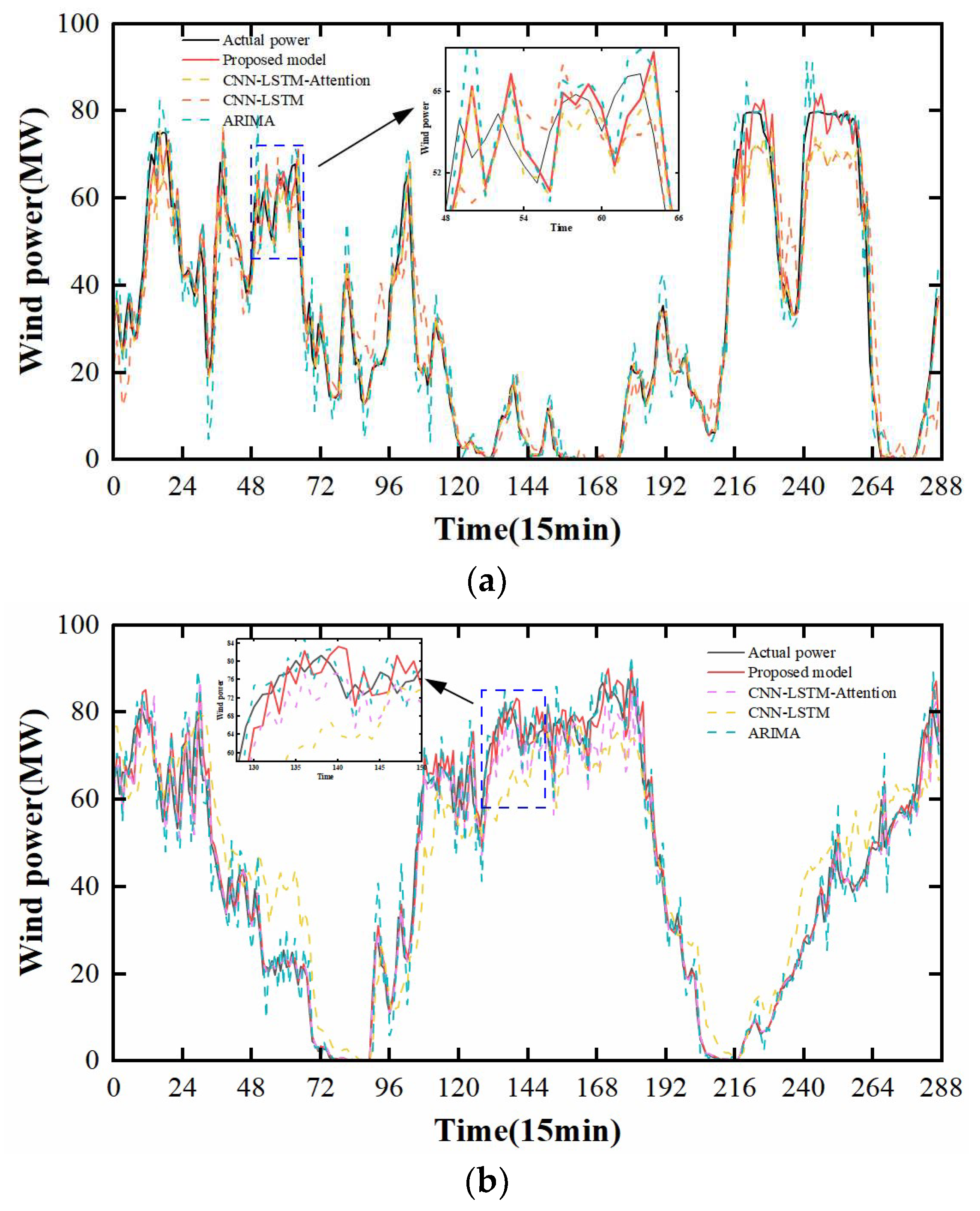
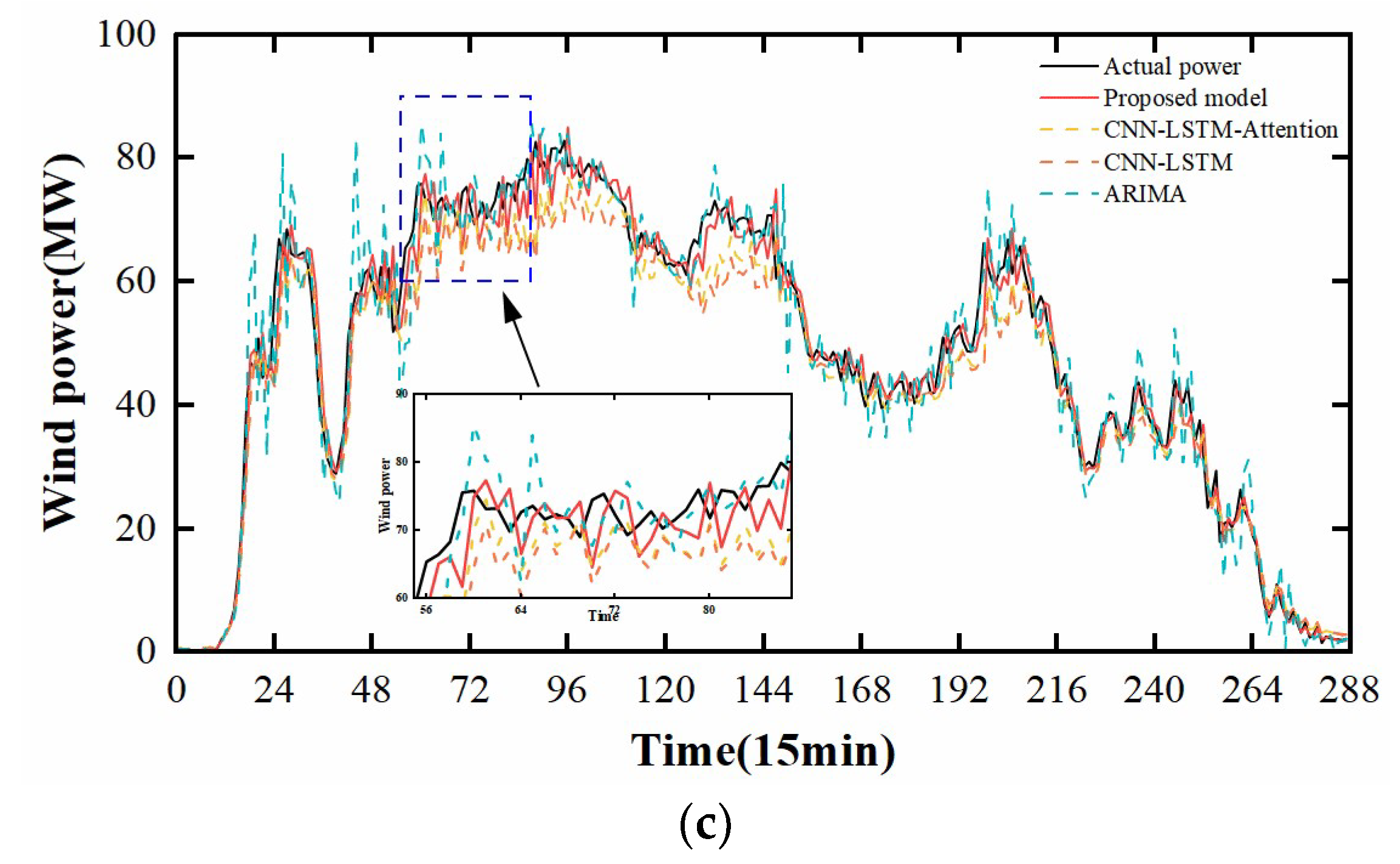
In order to analyze the accuracy and superiority of the proposed model’s performance, the model’s prediction accuracy is evaluated using the evaluation metrics in Equations (14)–(16). The CNN-LSTM-Attention, CNN-LSTM, and ARIMA models belonging to the traditional statistical methods are validated against the prediction models in this paper. Table 3 shows the prediction effect evaluation indexes of different prediction models in three wind farms. Figure 4 is the wind power prediction effect diagram of different models in three wind farms. In order to ensure fairness, the model runs 10 times to take the average value as the final result.
Table 3 shows the prediction performance evaluation summary of three different wind farms under different prediction models by using the MSE, MAE, and R2 three evaluation indexes. The average MSE values of the three wind farms in the proposed model and CNN-LSTM-Attention, CNN-LSTM, and ARIMA models are 23.086, 34.124, 67.183, and 42.411, respectively; the mean values of the MAE were 3.237, 4.232, 6.406, and 4.442, respectively. The mean values of R2 were 0.96, 0.941, 0.89,7 and 0.930, respectively. From the comparison in the table, it can be observed that the proposed model has smaller MSE and MAE values than other conventional models, indicating that the proposed model achieves smaller prediction errors compared to the control model. Meanwhile, the R2 value of the proposed model is closer to 1, which indicates that the prediction effect is better than the control model. Here, it is found that the prediction accuracy of the ARIMA model exceeds that of some of the prediction models, and the main reason for this is that the model can track the wind power better in shorter time scales, but with the increase in time scales, its prediction accuracy decreases sharply compared with other deep learning models, which is no longer shown due to the limited space in this paper [40]. Overall, the proposed model has better prediction accuracy.
Figure 4 is the 72 h prediction results of three wind farms in China under different prediction models. The environment built by the three wind farms is quite different, which can better compare the prediction performance of different models. Comparison between deep learning models reveals that the model proposed in this paper has better wind power tracking ability. Comparison with the ARIMA model reveals that the prediction results of the ARIMA model fluctuate the most during the time period when wind power fluctuates, mainly because the model finds it difficult to deal with non-stationary and complex non-linear time series data. It can be seen that the wind power prediction curves of the proposed model in different wind farm environments are closer to the actual power curve, which shows the effectiveness and stronger generalization of the model’s prediction.
The main reason for the error is that the wind farm environment is a complex coupling environment and the environmental monitoring equipment can not completely monitor all the changes in the whole wind farm, and systematic, random, and human errors existing in the sensor monitoring process are inevitable, which are objective reasons that may lead to the existence of errors. In the daily operation of a wind power plant, the reliability of operation equipment and monitoring equipment should be regularly checked so as to reduce the occurrence of errors, limit the occurrence of wrong operation instructions for the power’s plant dispatching personnel due to wrong operation data, and improve the stable operation of the wind power plant.
Through the above comparative analysis, the proposed model has achieved satisfactory results. By analyzing all the results, it is summarized as follows:
  • The model proposed in this paper has better prediction performance. Experiments show that the integrated prediction algorithm proposed in this paper can extract the spatial-temporal correlation of different input features more deeply and obtain the model output with higher accuracy. The possible reason is that the integrated model combines the advantages of multiple single models, which makes the model have better feature extraction ability and nonlinear mapping ability and improves the overall data extraction ability and prediction performance of the model.
  • Compared with other models, the graph network model with attention mechanism can better express the relationship between different input feature nodes through self-learning so that the model has better generalization performance. Compared with other models, it has stronger spatial-temporal feature extraction ability, which confirms the effectiveness of the model’s prediction method.
In summary, the model proposed in this paper meets the requirements of accuracy, and the prediction accuracy is better than the existing prediction model. It has great potential in improving the operating efficiency and profitability of wind energy systems.

5. Model Interpretability

The introduction of multiple attention mechanisms provides interpretable capabilities for time series prediction models. In order to verify the rationality and effectiveness of the explanatory ability of the model proposed in this paper, it will be analyzed from the time dimension and the spatial dimension, and the rationality of the multi-dimensional explanatory results will be verified by combining expert knowledge. Time dependence and spatial dependence is a relative concept. Among them, temporal interpretability pays more attention to the learning ability of historical time changes during training, while spatial interpretability pays more attention to the spatial correlation between features.

5.1. Interpretability in Time Dimension

Increasing the attention mechanism of the time dimension in the model helps to observe the dependence of the model on different times. In this paper, the moving window size is set to 12, which means that the wind power at a future time point is predicted by the data of the 12 points in the history. By extracting the attention mechanism weight of the model at the 5th, 40th, and 100th iterations, the dependence of the model on the time dimension is observed. As shown in Figure 5, the vertical axis of the graph represents the different prediction time in the prediction result, and the horizontal axis represents the weight of the observed historical moment over the prediction step. It can be observed that with multiple iterative training of the model. The model pays more attention to the time step closer to the predicted target time. Due to the strong randomness and volatility of the wind speed affecting the wind power, the difference in the characteristics of the different times is large, so the data at closer times have stronger references. The interpretable heat map of the model in the time dimension is consistent with prior knowledge.

5.2. Interpretability in Spatial Dimension

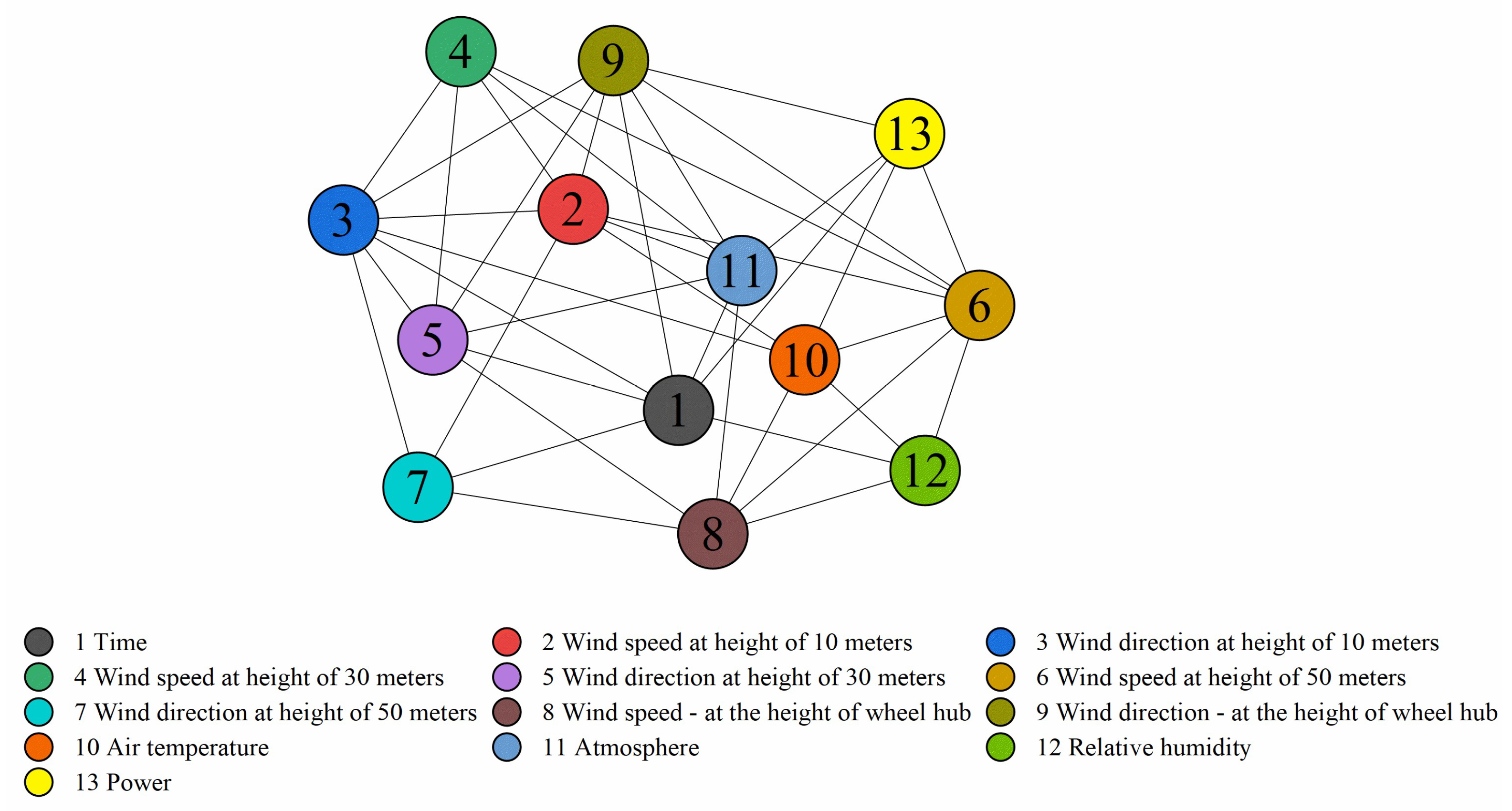
Wind farms collect a large number of different historical features through sensors, but not all features may be directly related to wind power output. Therefore, this paper introduces different historical features into the graph neural network model to mine hidden spatial dependencies and also initiates ‘noise reduction’ processing on many features, making the model more robust. At the same time, the graph neural network uses the gradient descent method to learn by itself, and the graph structure information also shows the network’s understanding of spatial dependencies. The connection between nodes can be used as the result of model space interpretability. At the same time, it should be noted that since undirected graphs are used in this study, the connections between nodes can only represent the correlation between the features learned by the model, but no direct causal relationship can be determined.
In Figure 6, we can see that the features directly connected to the wind power node include time, wind speed at height of 50 m, air temperature, atmosphere, and wind direction at the hub height. According to expert knowledge, the change in temperature is a prerequisite for the change in local air pressure, and the pressure gradient force is the main driving force of wind speed. This force is generated by the pressure difference between the two positions and determines the direction of the wind. At the same time, the greater the pressure difference, the greater the wind. Because wind power is proportional to the third power of wind speed, wind speed is the most important factor affecting wind power generation. In order to generate as much power as possible, the wind turbine will make the wind turbine always face the wind through the wind measurement system in the cabin position. It is worth noting that the model here pays more attention to the wind speed at a height of 50 m, perhaps because the model pays more attention to the influence of the wind speed blowing towards the fan blades. At the same time, the wind speed at the height of 50 m is directly related to the wind speed at the hub height. The proposed model shows that the direct influencing factors of wind farm output are consistent with expert knowledge, and the reliability and rationality of the model are verified.

6. Conclusions and Future Work

This paper proposes an interpretable wind power short-term prediction model using deep graph attention networks. Specifically, wind power prediction is a time series problem, and the prediction itself largely depends on the input of multiple historical characteristics of wind farms. Different time features have different volatilities, and different features contain the spatial attributes of the wind farm, which are the inherent attributes of the target wind farm. Therefore, digging into the spatial-temporal characteristics of the wind farm is key to improving the accuracy of wind power prediction. The simulation comparison shows that
  • The model proposed in this paper is higher than the existing model in terms of the prediction accuracy, indicating that the model can more fully mine the spatial-temporal characteristics of the multi-factor characteristics of the target wind farm.
  • Under the complex meteorological conditions of wind power generation, the GAT can better aggregate and extract the key information of the original multi-input features and more deeply mine the spatial-temporal characteristics of the original features. It provides a new solution to solve the problem of multi-factor feature modeling for wind power prediction.
  • The model applies the attention mechanism to obtain interpretability from the spatial and temporal dimensions. Because of the strong volatility of wind power, the long-term information has little reference significance to the model, which leads to the model paying more attention to the time step close to the predicted target time. The graph node structure self-learnt by the graph network structure shows the feature information that wind power prediction pays more attention to. The visualization of model details and the more transparent operation mechanism also bring greater application value to power grid operation scheduling and wind power consumption.
In future work, because the wind power output is affected by uncertain factors such as meteorology and the environment, it has higher randomness and volatility. Based on the high deterministic prediction accuracy of the model in this paper, wind power output probability prediction modeling will be carried out in the future to further improve the reliability of the prediction results.

Author Contributions

Conceptualization, J.Z.; Methodology, H.L.; Software, H.L.; Validation, J.Z. and P.C.; Formal analysis, P.C.; Investigation, J.Y.; Resources, J.Z.; Writing—original draft, H.L.; Visualization, J.Y. All authors have read and agreed to the published version of the manuscript.

Funding

This work is supported in part by the National Key Research and Development Program Project (Grant number: 2019YFE0104800), the Scientific and Technological Innovation Team of Colleges and Universities in Henan Province (Grant number: 22IRTSTHN011), Scientific and Technological Research Project of Henan Provincial Department of Education (Grant number: 20A210027).

Data Availability Statement

The dataset used in this study is from the Renewable Energy Generation Forecasting Competition hosted by the Chinese State Grid in 2021.

Conflicts of Interest

The authors declare no conflict of interest.

Abbreviations

GNNGraph neural network
LSTMLong short-term memory
NWPNumerical weather prediction
RNNRecurrent neural network
CNNConvolutional neural network
GCNGraph convolutional network
GATGraph attention network
SCADASupervisory control and data acquisition
TCNTime convolutional network
GRUGated recurrent unit
ARIMAAutoregressive integrated moving average

References

  1. Moayyed, H.; Moradzadeh, A.; Mohammadi-Ivatloo, B.; Aguiar, A.P.; Ghorbani, R. A Cyber-Secure generalized supermodel for wind power forecasting based on deep federated learning and image processing. Energy Convers. Manag. 2022, 267, 115852. [Google Scholar] [CrossRef]
  2. Zhang, J.; Liu, L.; Liu, Y.; Zhu, Y.; Yan, J. Research on Robust Model Predictive Control Strategy of Wind Turbines to Reduce Wind Power Fluctuation. Electr. Power Syst. Res. 2022, 213, 108809. [Google Scholar] [CrossRef]
  3. Liu, H.; Duan, Z. Corrected multi-resolution ensemble model for wind power forecasting with real-time decomposition and Bivariate Kernel density estimation. Energy Convers. Manag. 2020, 203, 112265. [Google Scholar] [CrossRef]
  4. Xu, Y.; Jia, L.; Yang, W. Correlation based neuro-fuzzy Wiener type wind power forecasting model by using special separate signals. Energy Convers. Manag. 2022, 253, 115173. [Google Scholar] [CrossRef]
  5. Yan, J.; Zhang, J.; Liu, Y.; Han, S.; Li, L.; Gu, C. Unit commitment in wind farms based on a glowworm metaphor algorithm. Electr. Power Syst. Res. 2015, 129, 94–104. [Google Scholar] [CrossRef]
  6. Sun, S.; Wang, T.; Yang, H.; Chu, F. Condition monitoring of wind turbine blades based on self-supervised health representation learning: A conducive technique to effective and reliable utilization of wind energy. Appl. Energy 2022, 313, 118882. [Google Scholar] [CrossRef]
  7. Hoolohan, V.; Tomlin, A.S.; Cockerill, T. Improved near surface wind speed predictions using Gaussian process regression combined with numerical weather predictions and observed meteorological data. Renew. Energy 2018, 126, 1043–1054. [Google Scholar] [CrossRef]
  8. Allen, D.J.; Tomlin, A.S.; Bale, C.S.E.; Skea, A.; Vosper, S.; Gallani, M.L. A boundary layer scaling technique for estimating near-surface wind energy using numerical weather prediction and wind map data. Appl. Energy 2017, 208, 1246–1257. [Google Scholar] [CrossRef]
  9. Aasim; Singh, S.N.; Mohapatra, A. Repeated wavelet transform based ARIMA model for very short-term wind speed forecasting. Renew. Energy 2019, 136, 758–768. [Google Scholar] [CrossRef]
  10. Krishna Rayi, V.; Mishra, S.P.; Naik, J.; Dash, P.K. Adaptive VMD based optimized deep learning mixed kernel ELM autoencoder for single and multistep wind power forecasting. Energy 2022, 244, 122585. [Google Scholar] [CrossRef]
  11. Yesilbudak, M.; Sagiroglu, S.; Colak, I. A novel implementation of kNN classifier based on multi-tupled meteorological input data for wind power prediction. Energy Convers. Manag. 2017, 135, 434–444. [Google Scholar] [CrossRef]
  12. Zendehboudi, A.; Baseer, M.A.; Saidur, R. Application of support vector machine models for forecasting solar and wind energy resources: A review. J. Clean. Prod. 2018, 199, 272–285. [Google Scholar] [CrossRef]
  13. Shi, Z.; Liang, H.; Dinavahi, V. Direct Interval Forecast of Uncertain Wind Power Based on Recurrent Neural Networks. IEEE Trans. Sustain. Energy 2018, 9, 1177–1187. [Google Scholar] [CrossRef]
  14. Zhang, J.; Yan, J.; Infield, D.; Liu, Y.; Lien, F.-S. Short-term forecasting and uncertainty analysis of wind turbine power based on long short-term memory network and Gaussian mixture model. Appl. Energy 2019, 241, 229–244. [Google Scholar] [CrossRef]
  15. Lin, Z.; Liu, X. Wind power forecasting of an offshore wind turbine based on high-frequency SCADA data and deep learning neural network. Energy 2020, 201, 117693. [Google Scholar] [CrossRef]
  16. Cheng, L.; Zang, H.; Xu, Y.; Wei, Z.; Sun, G. Augmented Convolutional Network for Wind Power Prediction: A New Recurrent Architecture Design with Spatial-Temporal Image Inputs. IEEE Trans. Ind. Inform. 2021, 17, 6981–6993. [Google Scholar] [CrossRef]
  17. Nikodinoska, D.; Käso, M.; Müsgens, F. Solar and wind power generation forecasts using elastic net in time-varying forecast combinations. Appl. Energy 2022, 306, 117983. [Google Scholar] [CrossRef]
  18. Zhang, Y.-M.; Wang, H. Multi-head attention-based probabilistic CNN-BiLSTM for day-ahead wind speed forecasting. Energy 2023, 278, 127865. [Google Scholar] [CrossRef]
  19. Shan, Y.; Hu, J.; Shen, B. Distributed Secondary Frequency Control for AC Microgrids Using Load Power Forecasting Based on Artificial Neural Network. IEEE Trans. Ind. Inform. 2023, 1–11. [Google Scholar] [CrossRef]
  20. Yildiz, C.; Acikgoz, H.; Korkmaz, D.; Budak, U. An improved residual-based convolutional neural network for very short-term wind power forecasting. Energy Convers. Manag. 2021, 228, 113731. [Google Scholar] [CrossRef]
  21. Wang, C.-H.; Zhao, Q.; Tian, R. Short-Term Wind Power Prediction Based on a Hybrid Markov-Based PSO-BP Neural Network. Energies 2023, 16, 4282. [Google Scholar] [CrossRef]
  22. Zhu, Q.; Chen, J.; Shi, D.; Zhu, L.; Bai, X.; Duan, X.; Liu, Y. Learning Temporal and Spatial Correlations Jointly: A Unified Framework for Wind Speed Prediction. IEEE Trans. Sustain. Energy 2020, 11, 509–523. [Google Scholar] [CrossRef]
  23. Chen, Y.; Zhang, S.; Zhang, W.; Peng, J.; Cai, Y. Multifactor spatio-temporal correlation model based on a combination of convolutional neural network and long short-term memory neural network for wind speed forecasting. Energy Convers. Manag. 2019, 185, 783–799. [Google Scholar] [CrossRef]
  24. Liu, Y.; Qin, H.; Zhang, Z.; Pei, S.; Jiang, Z.; Feng, Z.; Zhou, J. Probabilistic spatiotemporal wind speed forecasting based on a variational Bayesian deep learning model. Appl. Energy 2020, 260, 114259. [Google Scholar] [CrossRef]
  25. Chowdhury, P.N.; Shivakumara, P.; Kanchan, S.; Raghavendra, R.; Pal, U.; Lu, T.; Lopresti, D. Graph attention network for detecting license plates in crowded street scenes. Pattern Recognit. Lett. 2020, 140, 18–25. [Google Scholar] [CrossRef]
  26. Huang, H.; Zhu, Q.; Zhu, X.; Zhang, J. An Adaptive, Data-Driven Stacking Ensemble Learning Framework for the Short-Term Forecasting of Renewable Energy Generation. Energies 2023, 16, 1963. [Google Scholar] [CrossRef]
  27. Severiano, C.A.; de Lima e Silva, P.C.; Weiss Cohen, M.; Guimarães, F.G. Evolving fuzzy time series for spatio-temporal forecasting in renewable energy systems. Renew. Energy 2021, 171, 764–783. [Google Scholar] [CrossRef]
  28. Yu, R.; Liu, Z.; Li, X.; Lu, W.; Ma, D.; Yu, M.; Wang, J.; Li, B. Scene learning: Deep convolutional networks for wind power prediction by embedding turbines into grid space. Appl. Energy 2019, 238, 249–257. [Google Scholar] [CrossRef]
  29. Chen, W.; Jiang, M.; Zhang, W.-G.; Chen, Z. A novel graph convolutional feature based convolutional neural network for stock trend prediction. Inf. Sci. 2021, 556, 67–94. [Google Scholar] [CrossRef]
  30. Zhao, L.; Song, Y.; Zhang, C.; Liu, Y.; Wang, P.; Lin, T.; Deng, M.; Li, H. T-GCN: A Temporal Graph Convolutional Network for Traffic Prediction. IEEE Trans. Intell. Transp. Syst. 2020, 21, 3848–3858. [Google Scholar] [CrossRef]
  31. Tao, S.; Zhang, H.; Yang, F.; Wu, Y.; Li, C. Multiple Information Spatial–Temporal Attention based Graph Convolution Network for traffic prediction. Appl. Soft Comput. 2023, 136, 110052. [Google Scholar] [CrossRef]
  32. Zhang, J.; Meng, H.; Gu, B.; Li, P. Research on short-term wind power combined forecasting and its Gaussian cloud uncertainty to support the integration of renewables and EVs. Renew. Energy 2020, 153, 884–899. [Google Scholar] [CrossRef]
  33. Chen, J.; Zhu, Q.; Shi, D.; Li, Y.; Zhu, L.; Duan, X.; Liu, Y. A Multi-Step Wind Speed Prediction Model for Multiple Sites Leveraging Spatio-temporal Correlation. Proc. CSEE 2019, 39, 2093–2106. [Google Scholar]
  34. Yu, C.; Yan, G.; Yu, C.; Zhang, Y.; Mi, X. A multi-factor driven spatiotemporal wind power prediction model based on ensemble deep graph attention reinforcement learning networks. Energy 2023, 263, 126034. [Google Scholar]
  35. Abou Houran, M.; Salman Bukhari, S.M.; Zafar, M.H.; Mansoor, M.; Chen, W. COA-CNN-LSTM: Coati optimization algorithm-based hybrid deep learning model for PV/wind power forecasting in smart grid applications. Appl. Energy 2023, 349, 121638. [Google Scholar] [CrossRef]
  36. Sun, S.; Liu, Y.; Li, Q.; Wang, T.; Chu, F. Short-term multi-step wind power forecasting based on spatio-temporal correlations and transformer neural networks. Energy Convers. Manag. 2023, 283, 116916. [Google Scholar] [CrossRef]
  37. Wang, C.; Tian, R.; Hu, J.; Ma, Z. A trend graph attention network for traffic prediction. Inf. Sci. 2023, 623, 275–292. [Google Scholar] [CrossRef]
  38. Bentsen, L.Ø.; Warakagoda, N.D.; Stenbro, R.; Engelstad, P. Spatio-temporal wind speed forecasting using graph networks and novel Transformer architectures. Appl. Energy 2023, 333, 120565. [Google Scholar] [CrossRef]
  39. Yuan, X.; Chen, C.; Jiang, M.; Yuan, Y. Prediction interval of wind power using parameter optimized Beta distribution based LSTM model. Appl. Soft Comput. 2019, 82, 105550. [Google Scholar] [CrossRef]
  40. Sun, R.; Zhang, T.; He, Q.; Xu, H. Review on Key Technologies and Applications in Wind Power Forecasting. High Volt. Eng. 2021, 47, 1129–1143. [Google Scholar]
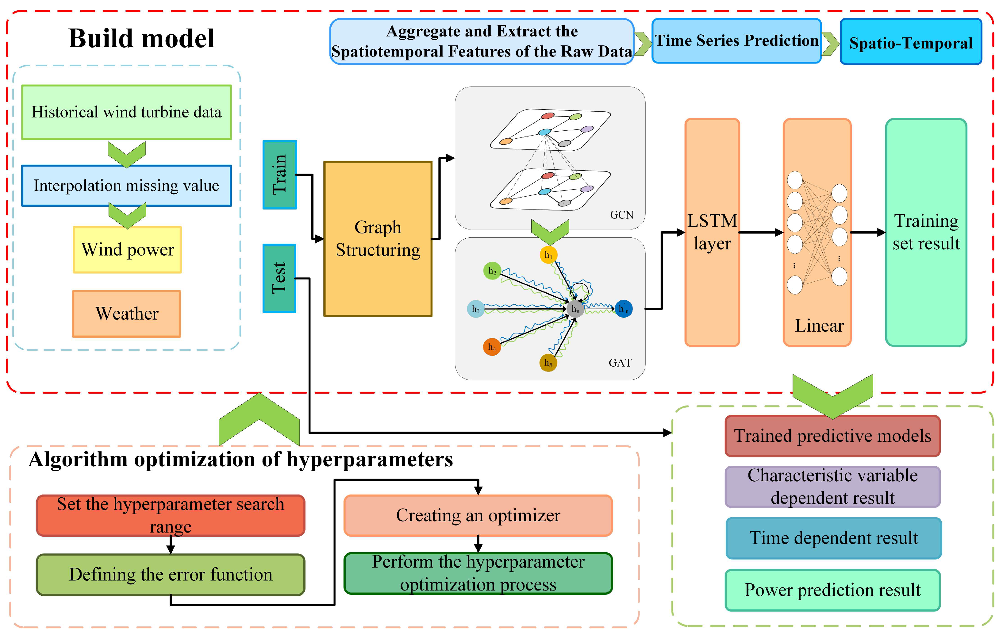
Figure 1. Spatial-temporal prediction model framework.
Energies 17 00384 g001
Figure 2. Long short-term memory unit.
Energies 17 00384 g002
Figure 3. Prediction model structure.
Energies 17 00384 g003
Figure 4. Wind power prediction results of wind farm. (a) Wind power station 1. (b) Wind power station 2. (c) Wind power station 3.
Energies 17 00384 g004aEnergies 17 00384 g004b
Figure 5. The change in attention weight based on different (5th, 40th, and 100th) iterations of time dimension (AC).
Energies 17 00384 g005
Figure 6. Model graph learning framework.
Energies 17 00384 g006
Table 1. Main parameters of wind farm.
Wind FarmGenerating Capacity (MW)Wind
Turbine Model
Capacity
(KW)
Hub Height
(m)
Rotor
Diameter
(m)
Number of Turbines
Farm site 175GW1500/85 1150085.087.050
24H93 L-2.0 2200085.593.012
Farm site 249.5UP86-1500 3150080.086.033
49.5UP82-1500 3150080.082.033
Farm site 396XE72 4200065.070.748
1 Xinjiang Goldwind Science & Technology Co., Ltd., a manufacturer from Beijing, China. 2 Haizhuang Windpower Co., Ltd., a manufacturer from Chongqing, China. 3 CSSC Guodian United Power Technology Co., Ltd., a manufacturer from Beijing, China. 4 XEMC Xiangtan Electric Manufacturing Co., Ltd., a manufacturer from Xiangtan, China.
Table 2. Wind farm statistics: variables, mean, variance, minimum and maximum.
StatisticsWind Speed—Height 50 m
(m/s)
Wind
Direction—Height 50 m
(◦)
Wind Speed—Height of Wheel Hub
(m/s)
Wind
Direction—Height of Wheel Hub
(°)
Air
Temp.
(°C)
Relative
Humidity
(%)
Farm site 1Mean6.169221.8686.376216.9868.54337.581
Std.3.87483.0923.90885.4013.36818.896
Min.0.0000.0000.0000.000−24.1311.502
Max.29.678358.93330.247358.50036.13093.120
Farm site 2Mean4.933143.0195.231179.94917.51158.809
Std.3.24193.3213.299110.1239.83823.501
Min.0.0000.0000.0000.000−14.273.437
Max.21.836360.036.920360.036.32100.0
Farm site 3Mean7.43687.7788.14594.14521.15878.649
Std.3.59289.1353.79791.2946.41610.883
Min.0.0000.0000.0000.0000.0000.000
Max.21.81360.023.82360.037.1399.38
Table 3. The evaluation index values of different prediction models in three wind farms.
Farm SiteModelMSE (MW)MAE (MW)R2
Site 1Proposed model21.8232.8080.962
CNN-LSTM-Attention29.5273.3890.949
CNN-LSTM51.3295.8990.901
ARIMA43.9764.5170.931
Site 2Proposed model26.7923.6910.951
CNN-LSTM-Attention33.4594.9260.934
CNN-LSTM102.9068.3010.864
ARIMA40.3384.4860.925
Site 3Proposed model20.6423.2120.968
CNN-LSTM-Attention39.3864.5310.939
CNN-LSTM47.3155.0190.927
ARIMA42.9194.3240.935
Disclaimer/Publisher’s Note: The statements, opinions and data contained in all publications are solely those of the individual author(s) and contributor(s) and not of MDPI and/or the editor(s). MDPI and/or the editor(s) disclaim responsibility for any injury to people or property resulting from any ideas, methods, instructions or products referred to in the content.