A Review of Fast Power-Reserve Control Techniques in Grid-Connected Wind Energy Conversion Systems

Abstract

Grid-connected power-converter-interfaced systems have been sharing the responsibility of grid generation alongside conventional synchronous generators. However, these systems lack spinning reserves, leading to a decrease in system inertia and resulting in more pronounced frequency deviations during power imbalances. Therefore, grid codes require the active involvement of wind energy conversion systems in frequency control, aiming to constrain the frequency and rate of change of frequency variations within predefined limits. This paper reviews fast power-reserve control techniques without energy storage in wind energy conversion systems that do not depend on frequency or rate of change of frequency values. The resulting effects on system frequency, energy production, mechanical loadings, and electrical loadings are assessed. The techniques are classified in the maximum-power point-tracking region according to the power function during the transient response, such as constant, speed-, time-, or mechanical power-dependent methods. Both overproduction and underproduction stages are considered. Certain techniques are tested on simulation grids that include either hydro or no-reheat steam generators, followed by a comparative analysis.

1. Introduction

The sustainable energy transition comprises the reduced use of overall energy and a higher proportion of energy generation from renewable resources [1]. Environmental issues have been emerging; therefore, there are increasing demands for renewable energy generation, reducing greenhouse gas emissions, implementing demand response strategies, and conservating energy [2]. Global efforts have already begun to take action, exemplified by the Paris Agreement in 2016, which requires 186 countries to present more aggressive plans for reducing emissions [3]. This has spurred the development of green energy systems, which rely on renewable-based sources, energy storage, and electric vehicles. These systems require smart control systems and real-time monitoring to operate optimally [4]. Consequently, it has become essential to shift our mindset from the operation of conventional power systems to a new paradigm. This new paradigm includes non-linear power flow, distributed generation resources, diverse grid ancillary service requirements, and the integration of traditional transmission system regulation into distribution networks [5]. These novel challenges have motivated recent studies on technical aspects of sustainable energy systems [6].

The recent growth of non-synchronous renewable energy sources has been driving the development toward sustainable energy generation [3]. However, it necessitates modifications in power system structures due to the lower capacity generation of renewable units compared to traditional power plants, their integration with power-electronic converters [4], and their diverse characteristics [5]. The high penetration of intermittent renewable resources poses challenges to grid operations, including (i) transmission systems: good wind and large-scale solar sites may be located in areas far from transmission systems or with limited transmission capacity; (ii) distribution systems: residential solar generation leads to new power flow patterns, requiring changes in protection and control strategies; (iii) interconnection standards: these standards are related to power factor correction and low-voltage ride-through capability; (iv) operational challenges: these arise due to the intermittent nature of wind and solar generation and (v) forecasting and scheduling: these are necessary to maintain a reliable dispatchable power reserve [2].

The power balance of electric grids is constantly affected by load disconnections, variations in generated power, device failures, and grid faults [7]. Power imbalances are naturally addressed by synchronous generators, as they act as energy buffers by delivering additional power when needed or absorbing surplus energy in the form of kinetic energy [8], which results in frequency variations. After a few seconds, the primary controllers take action, adjusting power generation to limit the frequency deviations, often implemented using a droop controller. This controller requires a primary active power reserve from the generated power. However, these characteristics are partially lost when connecting power inverters interfaced with the grid.

In the context of the ongoing energy transition, power-electronic systems play a crucial role in facilitating the integration of energy from renewable sources into the electric grid [9]. These systems operate alongside traditional synchronous generators to supply power to the loads. However, they do not have the inherent ability to absorb or release energy to counteract grid frequency variations, a challenge posed by the reduced system inertia and increased frequency excursions in modern grids [10]. This situation can potentially jeopardize the security of synchronous generators and may necessitate load-shedding schemes due to high rates of change of frequency (ROCOF) [7]. This underscores the importance of incorporating inertia capacity or grid-frequency-based control mechanisms to uphold grid frequency stability [11]. Therefore, power-electronic-based generation systems should be designed to provide essential ancillary services, including frequency regulation and voltage control [12]. Consequently, power-electronic converters interfacing with renewable power generation can have a significant impact on system stability in various aspects, such as rotor angle and small-signal stability, voltage stability, frequency stability, sub-synchronous resonance, and oscillatory stability [13].

Low inertia systems have been experiencing frequency collapses due to the lack of sufficient inertia and frequency control, underscoring the need for dedicated efforts to enhance frequency stability in modern power systems [14]. The South Australia blackout event stands out as the first known incident in a grid predominantly reliant on renewable energy sources, with approximately 50% renewable power penetration. Its primary cause is possibly attributed to high ROCOFs and frequency deviations. Implementing frequency control support in wind energy conversion systems could offer a cost-effective solution to prevent such events [15]. In California, a power outage of 900 MW of solar generation was partially attributed to the erroneous operation of the phase-locked loop used for estimating frequency [16]. Additionally, other challenges may arise during extreme cold weather conditions, as exemplified by the 2021 power crisis in Texas. During this event, gearboxes froze and blades became covered in ice, rendering power generation unviable. Consequently, the available stored gas was insufficient to compensate for the energy deficit [17]. The outage events related to frequency instability in high non-synchronous renewable grids are used to update grid codes regarding the frequency control of wind power plants (WPP), as verified in [18] for 11 countries. These grid codes require a continuous operation of WPPs over a specific frequency range and a primary frequency response via droop control. However, few grid codes have already demanded the inertial response of WPPs, which may be revised in the following years, given the increasing use of non-synchronous generation and the consequent reduction in the grid inertia.

Wind energy conversion systems (WECS) with full-scale power converters have become the prevailing trend in new wind farms, particularly in offshore installations [19]. These systems are typically categorized as Type-IV WECS and can utilize either a squirrel-cage induction generator or a synchronous generator (permanent magnet or wounded rotor) [20]. Among these options, the permanent magnet synchronous generator (PMSG) can be assembled with a high pole number, enabling operation at low or medium speeds. This reduces the speed ratio of the gearbox or even eliminates the need for it, allowing for direct-drive operation [21]. The energy generated is typically delivered to the grid through a back-to-back converter topology, consisting of a generator-connected rectifier, a DC-bus, and a grid-connected inverter [22]. This configuration, with a DC-voltage link, facilitates dynamic decoupling between the rectifier and the inverter. This enables the generator to operate at frequencies different from the grid and, consequently, to track the maximum power point in accordance with the current wind speed [23]. Power is typically injected into the main grid using a grid following a control scheme. This technique uses a phase-locked loop (PLL) to synchronize the injected current with the grid voltage [24].

A characteristic of variable-speed wind turbines is the decoupling between generator speed and grid frequency. Therefore, the spinning and primary reserves from the variable-speed wind turbines are not naturally utilized to dampen frequency oscillations, unlike the grid-connected squirrel-cage induction generators employed in fixed-speed wind systems [25]. To provide frequency control support, various systems employ different approaches. Some mimic the behavior of synchronous generators using detailed mathematical models, while others apply the swing equation. Still, others enable non-synchronous renewable systems to respond to frequency changes on the grid [26]. The spinning reserve is provided through methods such as inertia emulation, synthetic inertia, or virtual inertia. In this context, inertia in future systems is understood as the ability to resist frequency changes through various forms of energy exchange, including synchronously connected machines (synchronous inertia) and converter-connected generation (virtual inertia). These mechanisms counteract the frequency fluctuations resulting from imbalances in power generation and demand [8], although being limited due to the limited rate of change in power [27], size of energy buffer, and computational delay [28].

Some reviews about frequency control support by wind energy conversion systems have already been published [29,30,31,32,33,34]. This paper diverges from previous reviews and focuses on strategies to improve frequency stability independent of grid frequency deviation or rate of change. 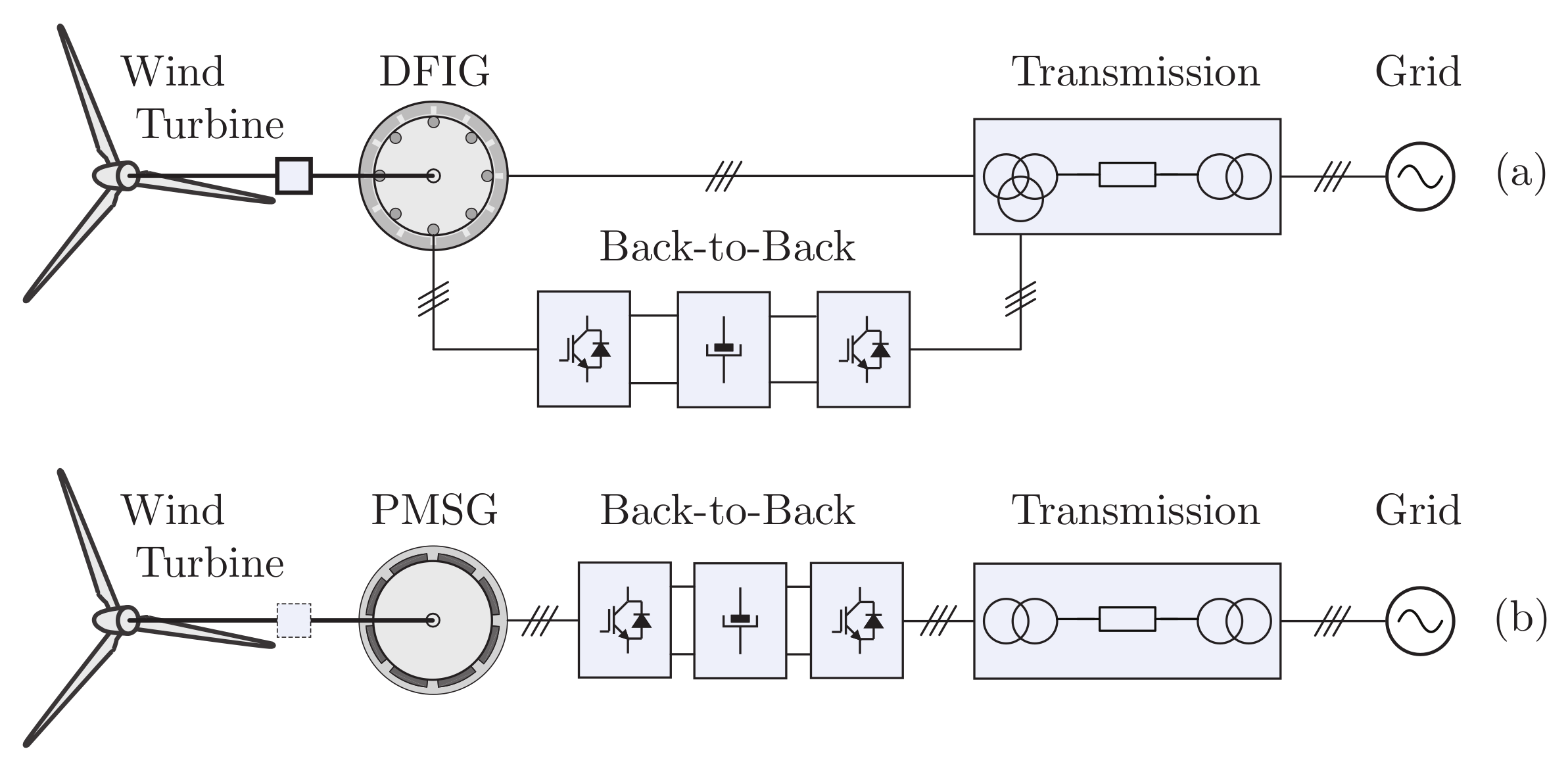Grid frequency information is employed solely for control triggering, and any anomalous event can be detected using a PLL or a dedicated event detector [35]. Commonly known as fast power reserve, this control technique can be implemented in both Type III and Type-IV wind energy conversion systems (illustrated in Figure 1a,b). In a Type-III WECS, the wind turbine is connected to a Doubly Fed Induction Generator (DFIG), which is connected directly to the grid in the stator and through a back-to-back converter in the rotor. This system can partially vary the rotor speed ($\pm 30\%$), and the power converter is rated at ($30\%$) of the generator power. Type-IV WECS typically employs a PMSG, with its stator connected to the grid through a power converter to decouple the generator and grid sides. This system requires full-scale power processing by the converter and can vary the rotor speed from zero to the rated speed ($100\%$) [23].

This review aims to analyze, categorize, and compare various fast power-reserve techniques employed to assist the grid during under-frequency events. The contributions of the paper include:

• Analysis of the concept of fast power-reserve techniques, the control implementation, and the typical dynamics in the wind turbine.
• Categorization of the methods based on the variables used to compute the power reference, such as rotor speed, time duration, and mechanical speed.
• Comparison of the impact of some methods in grids with different characteristics, such as hydro- and non-reheat-based generations, with a wind power penetration of $25\%$.
• Overview of recent challenges and trends in this research topic.

The paper is organized as follows: Section 2 presents the models for the wind energy conversion system, along with the main control loops; Section 3 introduces the concept of fast power reserve and some metrics used to assess its performance in the wind turbine; Section 4 lists and classifies the proposed methods of fast power reserve (FPR) in the literature, with detailed descriptions of some; Section 5 presents simulation results for selected control methods when connecting the wind turbine to either a hydro- or steam-based grid. Finally, Section 6 summarizes the main conclusions of the review.

2. Wind Energy Conversion System

Typical wind energy conversion systems include Doubly Fed Induction Generators (DFIG) or Permanent Magnet Synchronous Generators (PMSG). In a DFIG system, the rotor is connected to the grid through a partial-scale power converter (approximately 30% of the rated power) via slip rings, while the stator is directly linked to the grid. This configuration allows for the generator speed to be controlled by adjusting the active power of the power converter. On the other hand, PMSG systems are entirely decoupled from the grid by utilizing a full-scale power converter, enabling a wide speed variation of up to 100% [36]. Multipole generators are also available, providing an optional use of a gearbox [37]. Nevertheless, systems equipped with gearboxes may experience downtime due to gearbox faults. Consequently, many manufacturers choose to develop gearless (direct-drive) systems to enhance overall system reliability [38]. As a result of these distinctions, DFIG systems tend to be more cost-effective but may incur higher losses because of the gearbox. Conversely, PMSG systems tend to be more expensive due to the costs associated with the generator and converter. However, they offer the potential for the highest energy yield [39].

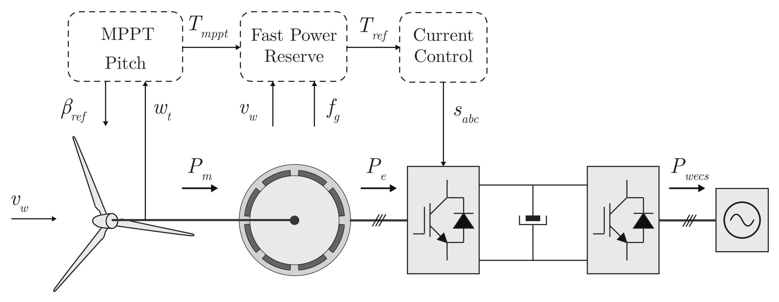
This paper focuses on Type-IV wind energy conversion systems as the basis for the analysis due to their prevalence in new installations [19] and the wide range of possible rotor operating speeds. A simplified control scheme for the wind generator with fast power reserve is illustrated in Figure 2, where the wind turbine, PMSG, and power converter are represented along the control loops. In steady-state operation, the wind turbine is controlled by the MPPT control in the medium wind region and by the pitch control in the high wind region. In this case, the torque reference from the MPPT ($T_{mppt}$) is limited to the rated power. The references of these controllers are combined with the fast power-reserve control reference, resulting in the generator torque reference $T_{ref}$. Subsequently, the generator current is controlled to obtain the reference torque. For the analyses presented in this review, both the current control and the power converter dynamics are neglected due to their significantly faster dynamics compared to the mechanical dynamics of the wind turbine and generator. Although a Type-IV WECS is considered, the results can be extended to Type-III WECS by limiting the maximum rotor speed variation, typically to $\pm 30\%$.

2.1. Wind Turbine Model

The power harnessed from the wind by the wind turbine is given as [40]:

$$P_m(v,\omega ,\beta )={\displaystyle \frac{1}{2}}\rho \pi R^2{C}_p(\lambda ,\beta )v^3,$$

(1)

here, $\rho$ represents air density, R denotes blade length, v signifies wind speed, $\omega$ stands for angular speed, $\beta$ represents the pitch angle, and $C_p$ is the power coefficient. Typically, this coefficient is expressed as an equivalent interpolated function obtained through model simulations or system identification [41]. In this article, the following expression for the power coefficient is utilized:

$$C_p(\lambda ,\beta )=0.5176\left({\displaystyle \frac{116}{{\lambda }_i}}-0.4\beta -5\right)e^{{\displaystyle \frac{-21}{{\lambda }_i}}}+0.0068\lambda ,{\lambda }_i={\left({\displaystyle \frac{1}{\lambda +0.08\beta }}-{\displaystyle \frac{0.035}{{\beta }^3+1}}\right)}^{-1},$$

(2)

here, the Tip–Speed Ratio (TSR), denoted as $\lambda$, represents the ratio between the linear speed at the blade tip and the wind speed [40]:

$$\lambda ={\displaystyle \frac{\omega R}{v}}.$$

(3)

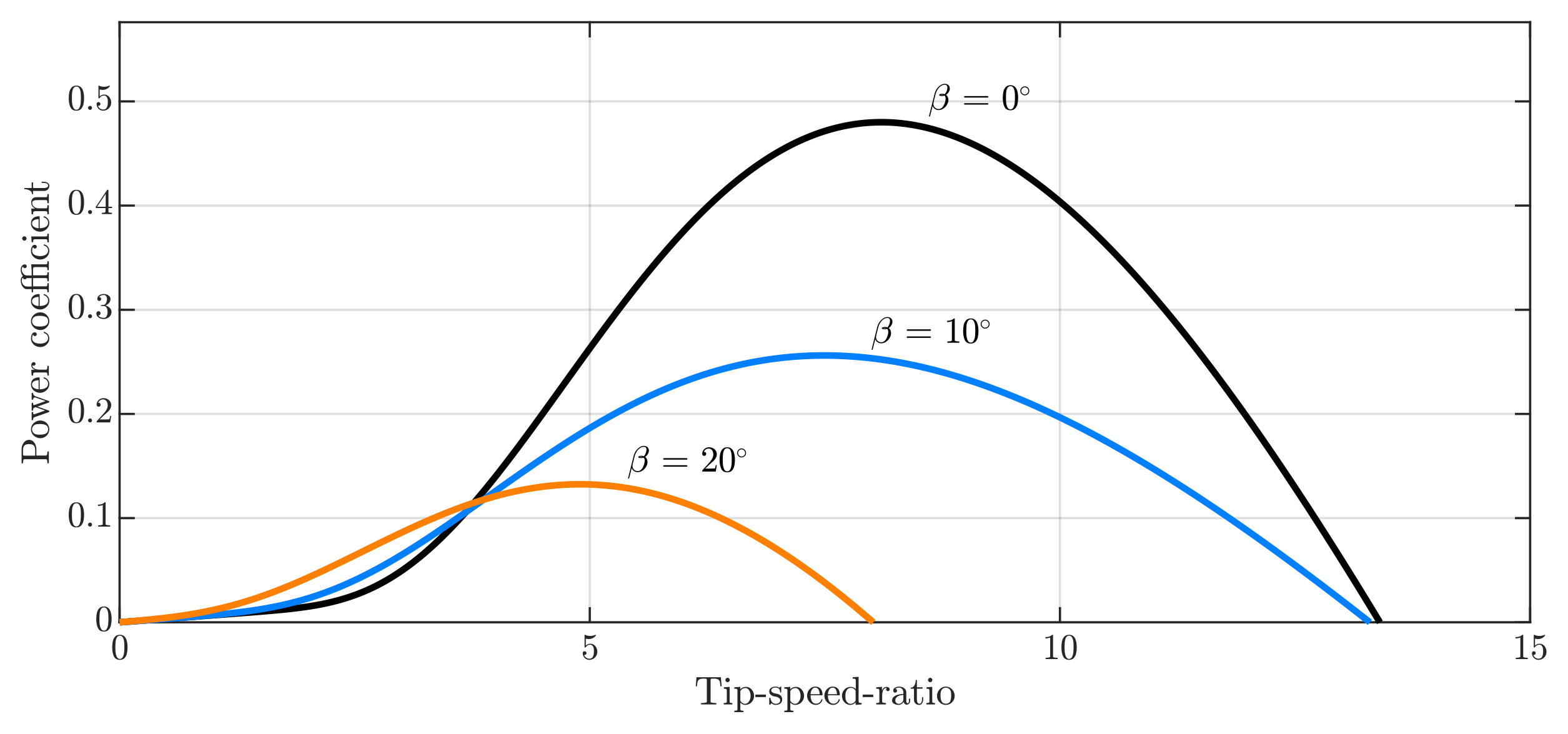
The power coefficient curves of the wind turbine as a function of the tip–speed ratio for different pitch angles are presented in Figure 3. It should be noted that, for each blade pitch angle, there exists an optimum TSR that results in the maximum power coefficient and, consequently, the highest harnessed power. The maximum power coefficient of 0.48 occurs when the blade pitch angle is 0$°$, and the tip–speed ratio is 8.1. The curves show that higher values of pitch angles reduce the power coefficient, except for low tip–speed ratio values.

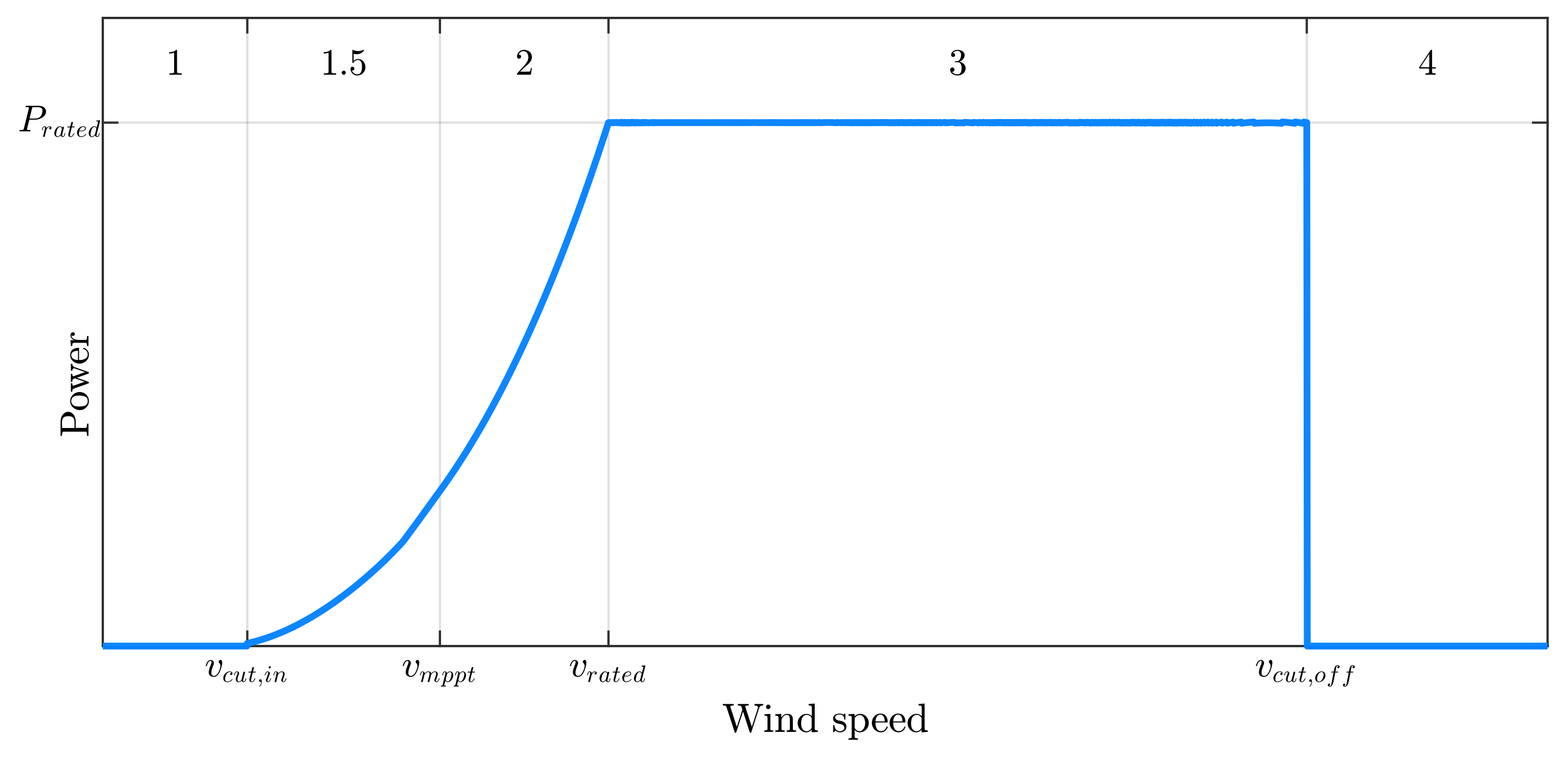
The power curve of the wind turbine as a function of wind speed in steady state is depicted in Figure 4. It can be characterized in four main regions of operation. In Region 1 ($v<v_{cut,in}$), the turbine is turned off because it cannot produce meaningful energy at low wind speeds. Region 1.5 ($v_{cut,in}\le v<v_{mppt}$) defines an operation with a fixed minimum angular speed, determined by mechanical resonance issues, where the pitch angle can be non-null to increase the generated power. Region 2 ($v_{mppt}\le v<v_{rated}$) is characterized by a variable rotor speed to obtain the maximum power coefficient and, consequently, maximum available power at a null pitch angle. In Region 3 ($v_{rated}\le v\le v_{cut,off}$) the turbine operates with rated rotor speed while limiting the generated power by increasing the blade pitch angle to prevent mechanical damage and overheating of the generator and power converters. In Region 4 ($v>v_{cut,off}$), the turbine is turned off to avoid high mechanical loads due to high wind speeds [42].

The turbine torque is calculated as the ratio of power to angular speed:

$$T_m(v,\omega ,\beta )={\displaystyle \frac{P_m(v,\omega ,\beta )}{\omega }}={\displaystyle \frac{1}{2}}{\displaystyle \frac{\rho \pi R^2{C}_p(\lambda ,\beta )v^3}{\omega }},$$

(4)

and the shaft dynamics are modeled as a single-mass system. Its equation is given by

$$J{\displaystyle \frac{d}{dt}}\omega =T_m-T_e-B·\omega ,$$

(5)

where B represents the friction coefficient, J denotes the equivalent moment of inertia combined from the wind turbine, shaft, and generator, and $T_e$ represents the electromechanical torque of the generator.

2.2. Maximum-Power Point Tracking

A minimum pitch angle value can be set for the low-wind region, where there is a minimum rotor speed constraint (Region 1.5). The minimum pitch is calculated based on the wind speed, and its objective is to maximize energy harvesting in low-speed regions [43]. To ensure that the wind turbine operates at its maximum power point for wind speeds in Region 2, a maximum-power point-tracking (MPPT) algorithm is employed. These methods are classified as indirect, direct, or hybrid power controllers. Indirect models search for the highest mechanical power, whereas direct models aim for the maximum electrical power. This study considers the Optimal Torque (OT) method, an indirect power controller known for its high reliability, simple implementation, and the fact that it does not require wind speed measurements [44]. This MPPT method sets the generator torque reference as

$$T_{mppt}\left(\omega \right)=\left({\displaystyle \frac{1}{2}}{\displaystyle \frac{\rho \pi R^5{C}_{p,opt}}{{\lambda }_{opt}^3}}\right)·{\omega }^2=K_{opt}·{\omega }^2.$$

(6)

3. Concept of Fast Power Reserve

The fast power-reserve method involves rapidly delivering or absorbing energy in response to frequency deviations to counteract the low inertial response. It may function either as a control logic based on the frequency deviation or a power reference set by a predetermined schedule [45]. Frequency control methods without deloading mean that the net power delivered to the grid over a short time period does not surpass the maximum possible power harvested from the wind turbine. Therefore, the WECS acts either on the torque reference of the synchronous generator or on the pitch angle reference during frequency deviations, with a limited duration defined by the mechanical constraints of the generator and the thermal limitation of the system.

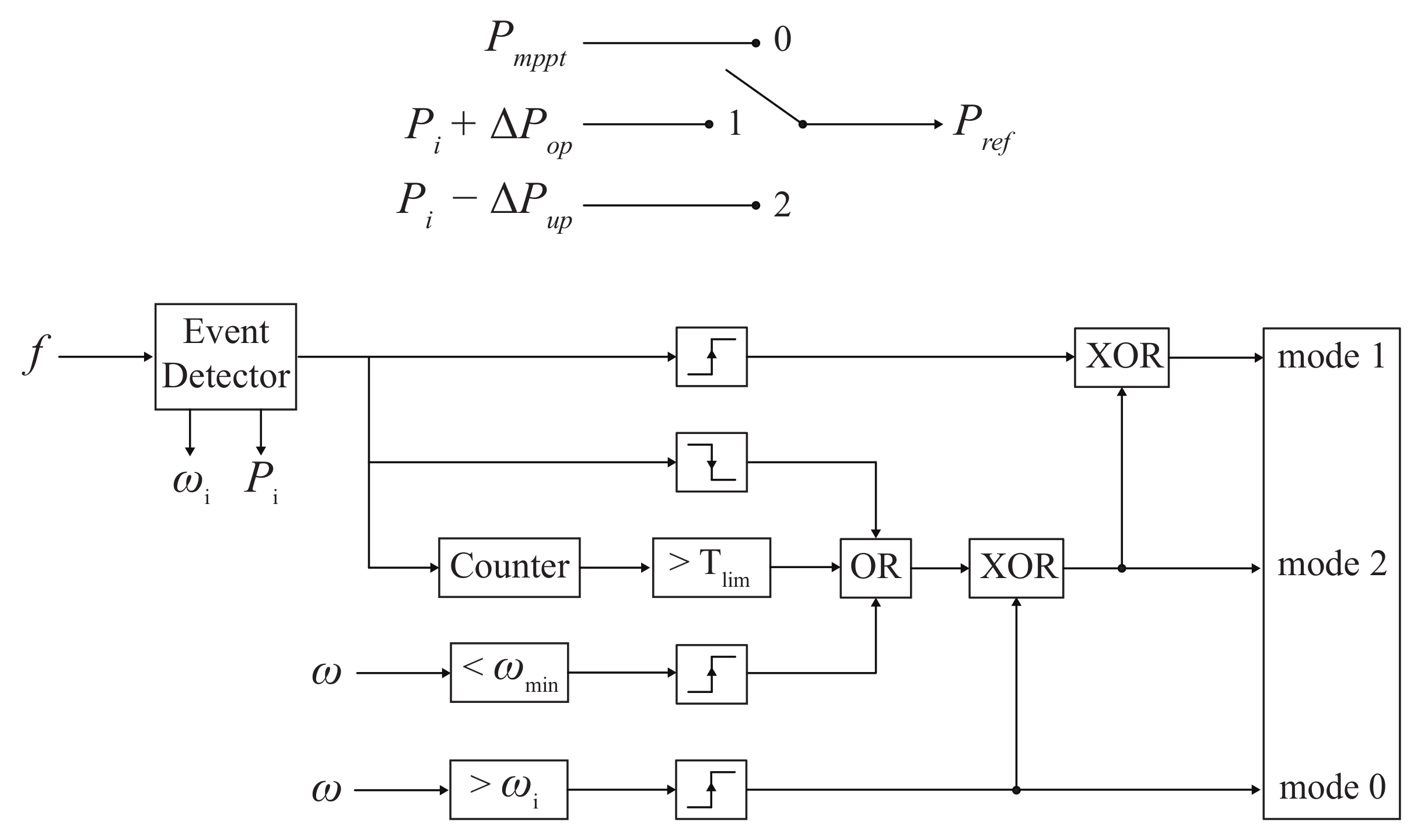
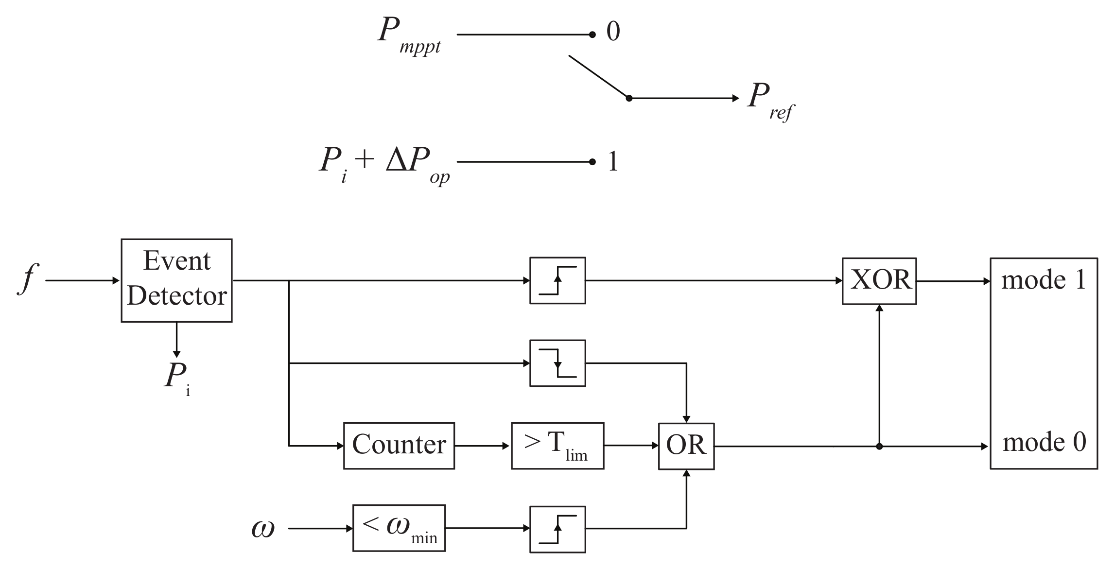
The idea of the fast power-reserve method is that the WECS, upon detecting a significant frequency deviation or rate of change in frequency, should increase its delivered power for a short period (on the order of seconds) to partially compensate for the grid power imbalance. The control scheme, based on the method proposed by [46], is illustrated in Figure 5. Initially, the power reference ($P_{ref}$) position is set to mode 0 (MPPT operation). Following the identification of an abnormal event, such as a high frequency deviation or a high rate of change in frequency, by the event detector, the controller sets the system to the first mode, also known as overproduction mode. During this mode, the power reference is the sum of the pre-event power $P_i$ and a predefined power increase $\Delta P_{op}$. Operation in this mode continues until one of three criteria is met: (i) event clearance (frequency and ROCOF are restored to allowable limits); (ii) dynamic time limit ($T_{lim}$) is exceeded; or (iii) minimum speed (${\omega }_{min}$) is exceeded. Subsequently, the second mode is activated, initiating the underproduction stage, where the power reference is the pre-event power ($P_i$) minus a predefined power decrease $\Delta P_{up}$. This mode continues until the turbine rotor speed returns to its pre-disturbance value (${\omega }_i$). At this point, the operating mode reverts to its initial state at the MPPT operation (mode 0), and the entire control scheme is reset to run again after an event detection.

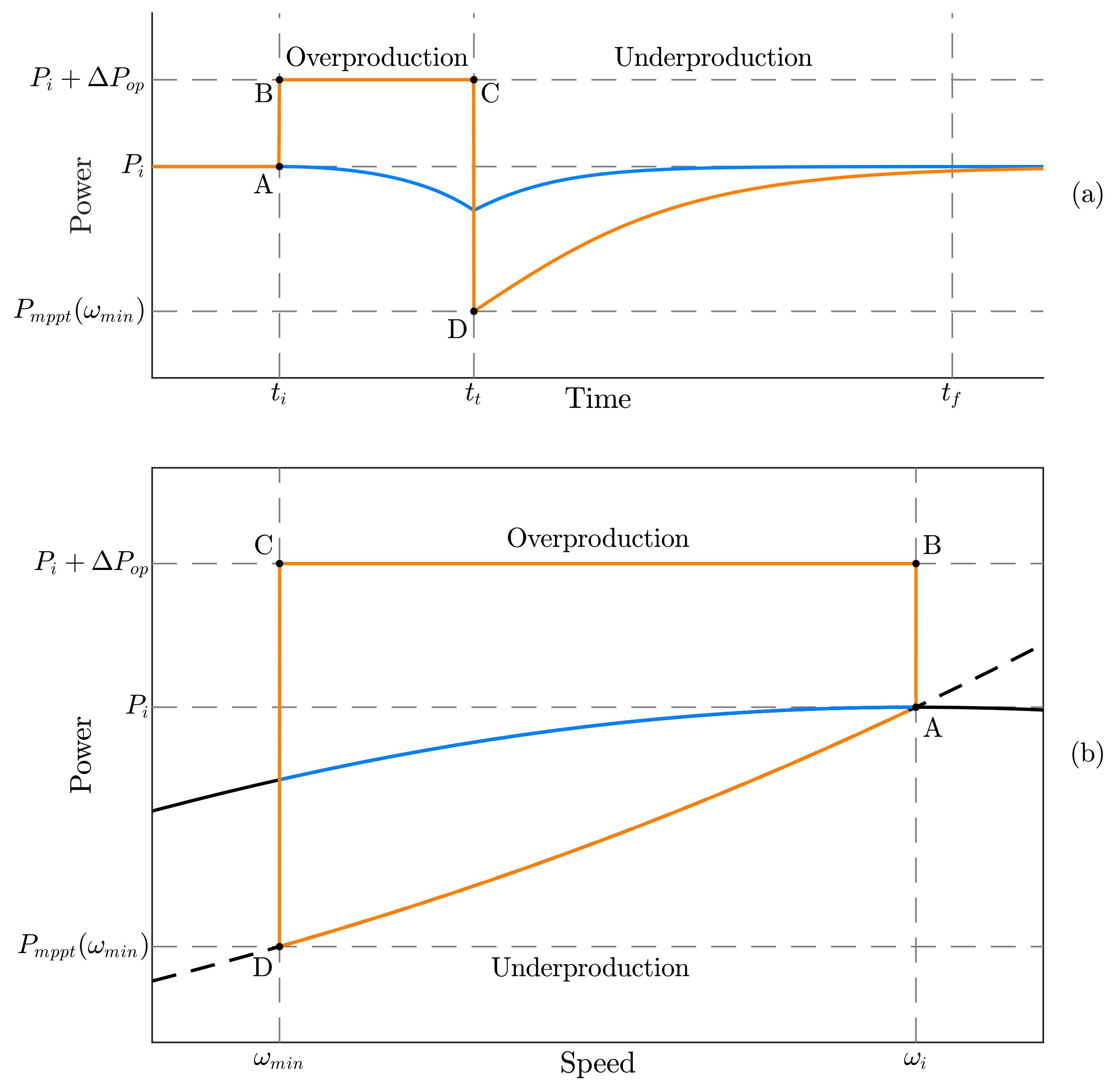
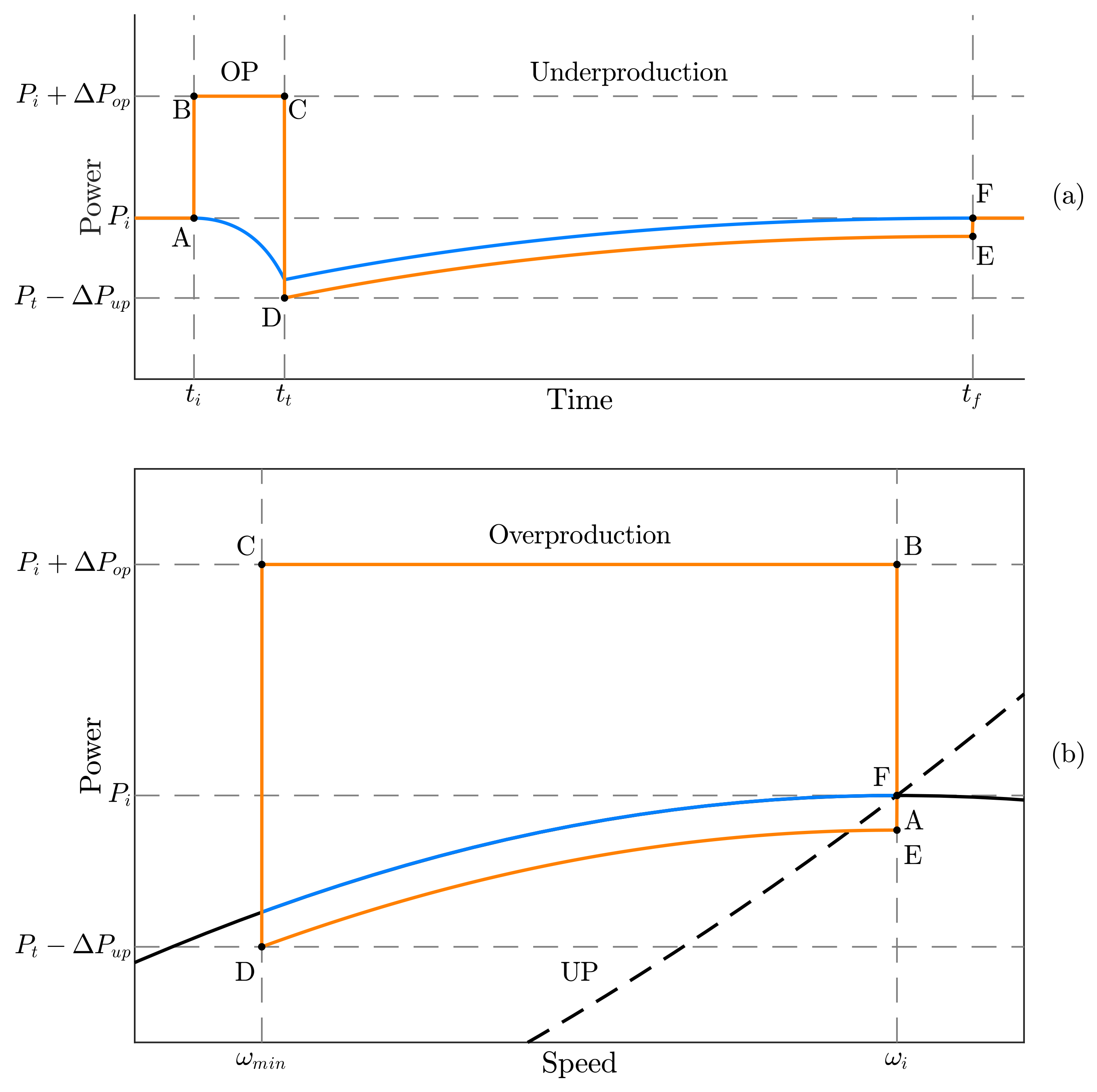
The conceptual waveforms for the controller proposed by [46] are presented in Figure 6, where the values of the generator and wind turbine powers as functions of time and generator speed during the fast power-reserve transient are depicted. In these waveforms, the generator power reference transitions from the MPPT method to a constant with a predetermined value for both over- and underproduction modes. It is important to note that during an under-frequency event, this constant power must surpass the pre-event power reference from the MPPT control to contribute to the grid frequency dynamics (overproduction mode).

The initial stage of the transient is the overproduction mode. Here, the generator power reference transitions from point ‘A’ to ‘B’, surpassing the maximum extracted power from the wind. This power difference is supplied by the stored kinetic energy in the wind turbine rotor, causing a slowdown (according to (5)) and deviation from the maximum power point, as shown in Figure 6b. The growing disparity between generator and wind turbine powers, as observed in the blue and orange curves during the overproduction mode ($t_i<t<t_t$) in Figure 6a, leads to an increase in the turbine’s deceleration. As the rotor speed decreases, the electromagnetic torque increases to maintain constant generator power. Besides the increased torque and the rotor deceleration, the power delivered to the grid is kept constant during the entire overproduction mode. This persists until the grid frequency returns to its limits or the wind turbine’s minimum speed constraint is reached [46]. In both cases, the wind turbine speed falls below its optimum level, necessitating acceleration to return to MPPT operation. Subsequently, the underproduction mode commences at the instant $t_t$, with the power reference transitioning from the overproduction power at point ‘C’ to the underproduction power reference at point ‘D’.

In the underproduction mode, the delivered power from the generator is constant, predetermined, and should be lower than the power harnessed from the wind [46]. Therefore, the mechanical power from the wind turbine is higher than the electromechanical power from the generator. Consequently, the wind turbine accelerates, increasing the TSR and the captured wind power (as seen in the blue curve of Figure 6a during the underproduction mode, where the mechanical power slowly converges to its initial value $P_i$). This mode persists until the wind turbine returns to its optimum speed ${\omega }_i$, at which point the controller switches from the underproduction power reference at point ‘E’ to the MPPT power reference at point ‘F’.

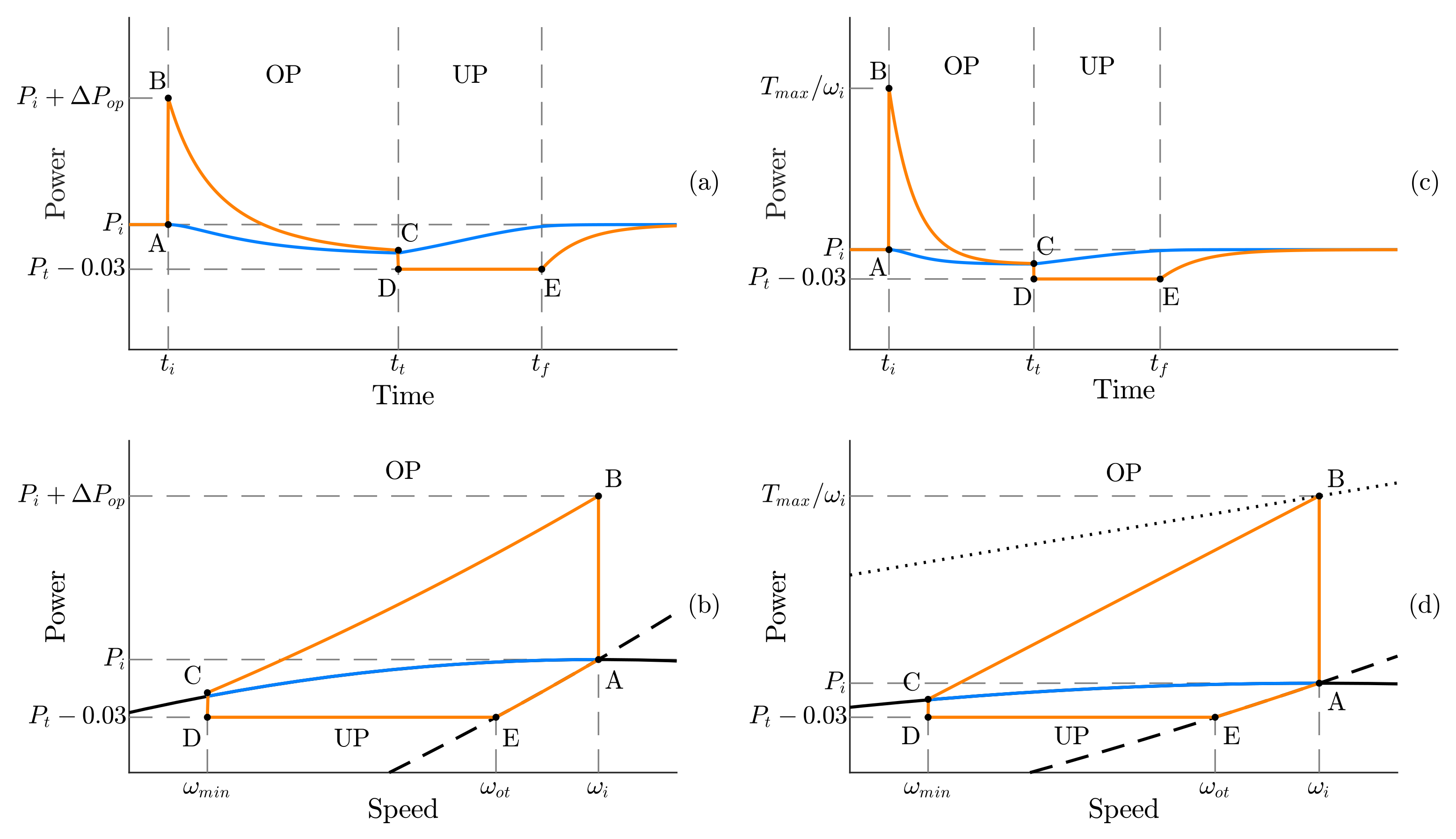
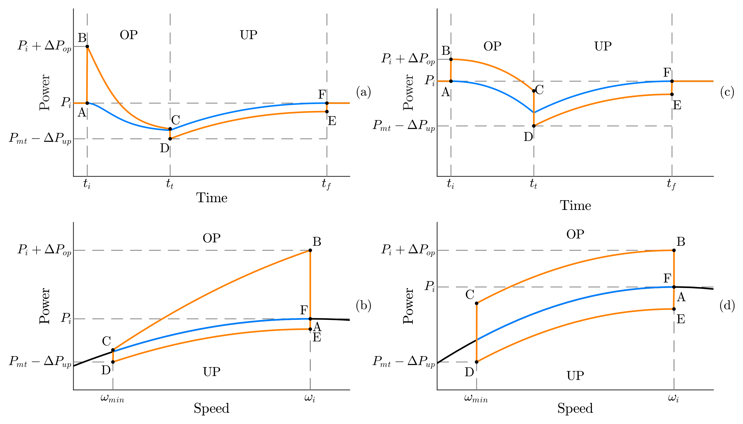
The method proposed and analyzed in [46] relies on predetermined constant power references for both over- and underproduction modes. However, it has some drawbacks, such as the significant steps in generator power references from points A,B, C,D, and E,F (as seen in the orange curve in Figure 6), along with high torque variations. Nonetheless, this method allows the computation of key factors essential for assessing a wind turbine’s ability to provide fast power reserves, including the maximum overload duration, the duration of angular speed restoration, and the total energy losses.

3.1. Maximum Overproduction Duration

The maximum duration of increased wind turbine power output is a crucial factor in assessing the frequency control capability of a wind turbine over a short period, as discussed in [46]. For an increase in delivered power, there is an operating limit determined by the minimum angular speed. From the wind turbine motion equation,

$$J{\displaystyle \frac{d}{dt}}\omega =T_m(v,\omega ,\beta )-T_e(\omega ,P_e),$$

(7)

where $T_e$ is the electromagnetic torque, $T_m$ represents the turbine (mechanical) torque, J is the moment of inertia and $\omega$ signifies the turbine angular speed. The equation can be rewritten by substituting torque variables with power and representing them in per-unit (pu) units as:

$$2H\omega {\displaystyle \frac{d}{dt}}\omega =P_m-P_e,$$

(8)

where $P_m$ denotes the wind turbine power, $P_e$ represents the generator power, and H is the inertia constant of the wind turbine, defined as

$$H={\displaystyle \frac{J{\omega }_b^2}{2P_b}}.$$

(9)

In this equation, ${\omega }_b$ represents the base angular speed, and $P_b$ is the base active power. The total overproduction duration $\Delta t_{over}$ can be determined by integrating (8) from the initial angular speed ${\omega }_i$ to the minimum allowable speed ${\omega }_{min}$:

$$\Delta t_{over}={\int }_{{\omega }_i}^{{\omega }_{min}}{\displaystyle \frac{2H\omega }{P_m-P_e}}d\omega .$$

(10)

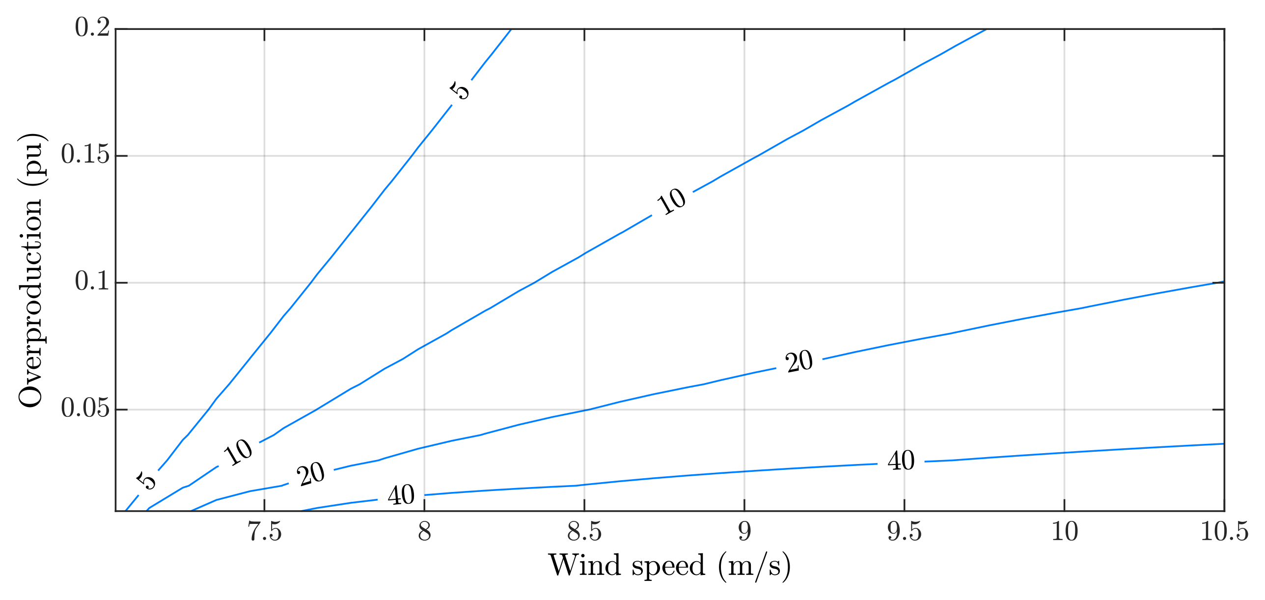
This equation demonstrates that the total overproduction duration depends on the system’s initial conditions and the generator power reference. Additionally, the duration is proportional to the equivalent inertia of the turbine, shaft, and generator. Figure 7 displays contour lines representing the maximum overproduction duration computed from (10) as a function of wind speed and overproduction power step $\Delta P_{op}$. Each line indicates the combination of both variables, resulting in the same overproduction duration. From the grid’s perspective, a longer overproduction duration is desirable, allowing sufficient time for conventional generators to increase their production and compensate for the power imbalance in the system. As expected, operation at higher wind speeds is associated with a greater capacity to deliver additional energy for a longer period.

3.2. Underproduction Duration

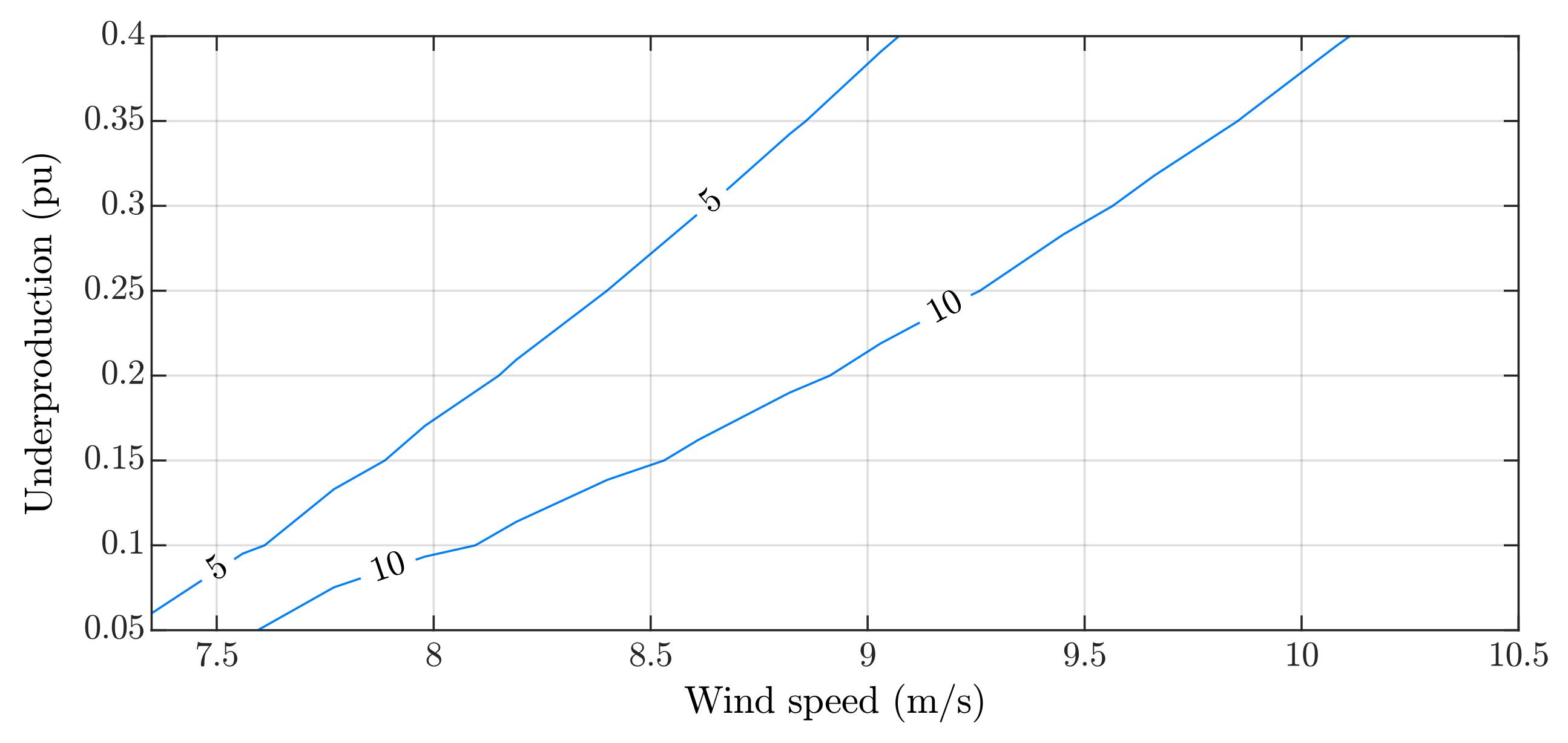
When transitioning away from the overproduction mode, restoring the wind turbine’s angular speed to its optimal value becomes necessary. The time required for this process depends on the initial operating point, wind speed, and the underproduction power reference. The duration to return the angular speed to its optimum value from the minimum rotor speed can be determined using the equation

$$\Delta t_{under}={\int }_{{\omega }_{min}}^{{\omega }_{opt}}{\displaystyle \frac{2H\omega }{P_m-P_e}}d\omega ,$$

(11)

here, the generator power is constant and predetermined. Figure 8 depicts contour lines representing the underproduction duration as a function of wind speed and underproduction power $\Delta P_{up}$. These lines illustrate the combinations of variables resulting in the same underproduction duration of 5 and 10 s. From the turbine perspective, a fast recovery with a high power reduction would be optimal for returning to MPPT operation. However, from the grid perspective, a high power reduction $\Delta P_{up}$ is undesirable, as it could potentially lead to a new frequency dip in the grid, necessitating an external power source to compensate for the power deviation. It is noteworthy that the recovery time increases with wind speed (due to the optimum angular speed) and decreases with a higher underproduction power reference. As the speed restoration is faster with a higher power deficit, a trade-off exists between the dynamic recovery of the wind turbine and the reduction in delivered power.

3.3. Energy Losses

The power over- and underproduction in the MPPT region deviates the wind turbine from its optimum angular speed, leading to reduced energy harnessed from the wind, as observed in the turbine power in Figure 6. The amount of unharvested energy depends on the initial operating point, the magnitude of power variation in both over- and underproduction modes, and the total duration. To assess energy efficiency during transient conditions at a constant wind speed, the following equation is employed:

$$\eta ={\displaystyle \frac{1}{P_{mi}·(\Delta t_{over}+\Delta t_{under})}}{\int }_{t_i}^{t_f}{P}_{m}dt,$$

(12)

where $P_{mi}$ is the ideal mechanical power harnessed from the wind, considering the MPPT operation. Since this control technique is intended for use during significant frequency deviations, the energy loss should be viewed as a trade-off for maintaining the system operating within operational constraints.

4. Fast Power-Reserve Techniques

Fast power-reserve techniques have been proposed to enhance the findings presented in [46], aiming for improvements in frequency dips, smoother power transitions, and limited torque levels. The references suggest novel over- and underproduction trajectories for the power reference as a combination function of constant values, rotor speed, time duration, and instantaneous mechanical wind turbine power.

Table 1. Fast power-reserve controllers as a function of wind turbine speed, time, grid frequency, and mechanical power. “✔” indicates inclusion in the power reference function, and “✗” indicates non-inclusion.

Reference	Overproduction Power Reference Function				Underproduction Power Reference Function
	Constant	Speed	Time	Mechanical Power	Constant	Speed	Time	Mechanical Power
[46]	✔	✗	✗	✗	✔	✗	✗	✗
[47]	✔	✗	✗	✗	✗	✔	✔	✗
[48]	✔	✗	✗	✗	✔	✗	✗	✔
[49] ${}^{\left(1\right)}$	✔	✗	✔	✗	✔	✗	✔	✗
[50]	✔	✗	✗	✗	✗	✔	✗	✗
[51]	✔	✗	✔	✗	✔	✗	✔	✗
[52]	✔	✔	✗	✗	✔	✔	✗	✗
[53]	✗	✔	✗	✗	✔	✔	✗	✗
[54] ${}^{\left(2\right)}$	✗	✔	✗	✔	✔	✔	✗	✔
[54] ${}^{\left(3\right)}$	✔	✗	✗	✔	✔	✔	✗	✔
[55]	✗	✔	✗	✗	✗	✔	✔	✗
[56]	✔	✔	✔	✗	✗	✔	✔	✗
[57]	✔	✔	✗	✗	✗	✔	✔	✗
[58] ${}^{\left(4\right)}$	✔	✗	✗	✗	✔	✔	✗	✗
[59]	✔	✔	✔	✗	✗	✔	✗	✗
[60]	✗	✔	✔	✗	✗	✔	✔	✗
[61]	✗	✔	✗	✗	✗	✗	✗	✗

⁽¹⁾ Time varying during the transition from overproduction to underproduction modes. ⁽²⁾ First method. ⁽³⁾ Second method. ⁽⁴⁾ Constant term is applied in the underproduction mode only for the fourth method.

chronologically lists the proposed control schemes from various references and categorizes them based on the power reference function. The only method utilizing a constant power reference in both overproduction and underproduction modes is from [46], as presented in Section 3. The subsequent subsections introduce other methods according to their categories in Table 1.

4.1. Methods Dependent on Rotating Speed

Methods dependent on rotating speed utilize a power reference function in either overproduction, underproduction, or both modes, which is dependent on the wind turbine’s rotor speed. This approach aims to minimize the impact of power reference steps on the generator output power and reduce the torque exerted on the shaft. Various methods proposed in the literature follow this principle. The comparison of power reference equations using only rotor speed as a variable is presented in

Table 2. Overproduction ($P_{op}$) and underproduction ($P_{up}$) power references for the speed-based functions aimed at releasing additional power and restoring the rotor speed, respectively.

Ref.	Overproduction	Underproduction
[50]	$P_{op}=P_i+\Delta P_{op}$	$P_{up}=P_{mppt}\left(\omega \right)$
[52] ${}^{\left(1\right)}$	$P_{op}=P_{mppt}\left(\omega \right)+\Delta P_{op}$	$P_{up}=\max (P^{*}-0.03,P_{mppt}\left(\omega \right))$
[53] ${}^{(1,2)}$	$P_{op}={\displaystyle \frac{P_{lim}\left({\omega }_i\right)-P_{mppt}\left({\omega }_i\right)}{{\omega }_i-{\omega }_{min}}}\left(\omega -{\omega }_{min}\right)+P_{mppt}\left({\omega }_i\right)$	$P_{up}=\max (P^{*}-0.03,P_{mppt}\left(\omega \right))$
[58] ${}^{(3,4)}$	$P_{op}=P_i+\Delta P_{op}$	$P_{up}=\max (P_{mppt}\left(\omega \right)+a{(\Delta \omega )}^2+b\Delta \omega +c,P_{mppt}\left(\omega \right))$
	$P_{op}=P_i+\Delta P_{op}$	$P_{up}=\max \left(P_{mppt}\left(\omega \right)+b\sqrt{1-{\displaystyle \frac{{\left(\Delta \omega +{\omega }_i-{\omega }^{*}\right)}^2}{a^2}}},P_{mppt}\left(\omega \right)\right)$
	$P_{op}=P_i+\Delta P_{op}$	$P_{up}=\max \left(P_{mppt}\left(\omega \right)-a^{\Delta \omega +{\omega }_i-{\omega }^{*}}+b,P_{mppt}\left(\omega \right)\right)$
	$P_{op}=P_i+\Delta P_{op}$	$P_{up}=\max \left(P_{mppt}\left(\omega \right)+a\Delta \omega +b,P_{mppt}\left(\omega \right)\right)$
[61] ${}^{\left(5\right)}$	$P_{op}=(P_i+\Delta P_{op})e^{-\frac{{\left(\omega -{\omega }_i\right)}^2}{2{\sigma }^2}}$	-

⁽¹⁾ $P^{*}$—Power at the end of the OP mode. ⁽²⁾ $P_{lim}\left({\omega }_i\right)$—Power at ${\omega }_i$ which results in the rated torque. ⁽³⁾ $a,b$ and c are determined by setting the initial underproduction power and the rotor speed to return to MPPT mode. ⁽⁴⁾ $\Delta \omega =\omega -{\omega }_i$ is the difference between the instantaneous and the initial rotating speed. ⁽⁵⁾ Reference [61] does not employ a specific underproduction power reference. It considers that it can slowly accelerate the rotor as the secondary frequency controller of the grid takes action.

. Notably, some methods only require known parameters and functions, such as the MPPT power reference and rated torque, while others necessitate the computation of parameters for the new trajectory function.

A straightforward modification of the method in [46] involves changing the constant power reference from the underproduction mode to the MPPT power curve reference [50] while retaining a constant power reference for the overproduction mode. This modification ensures convergence to the optimal rotor speed after the overproduction mode and eliminates the need to set an underproduction power reference. Notably, unlike the control scheme depicted in Figure 5 from [46], there is no requirement to record the rotor speed upon event detection, as demonstrated in the control scheme shown in Figure 9. In this method, the reference power ($P_{ref}$) initially matches the MPPT power reference ($P_{mppt}$) in the mode 0. When a frequency event is detected, the current power reference $P_i$ is saved and then added with an overproduction power $\Delta P_{op}$. Once the frequency event is resolved, the time limit is reached, or the rotor speed falls below the minimum value, the operation returns to mode 0, which is the underproduction mode with the MPPT reference.

The power curves against time and rotor speed are depicted in Figure 10a,b. It can be observed that the overproduction mode is consistent with the method shown in Figure 6. However, for wind speeds below the rated value, the significant variation in rotor speed still results in reduced energy harvesting and increased torque variations during the dynamic response in the overproduction mode. As highlighted in [50], a significant limitation of fast power reserve is the elevated torque levels, particularly at wind speeds slightly below the rated value. With a high power reference and decreasing rotor speed during the overproduction stage, torque sharply increases, posing a potential risk of damage to the wind energy conversion system. The novelty of this method lies in the underproduction mode, in which the rotor acceleration along the MPPT power curve is smoother, avoiding a third power step change as seen in E-F from Figure 6.

Both methods in [46,50] depend on fast power variation in the wind turbine, which might trigger another frequency deviation event during the transition from over- to underproduction modes (points C,D in Figure 6 and Figure 10). Consequently, alternative methods relying solely on rotor speed have been proposed to achieve a smoother power transition. In [52], a constant power reference is introduced alongside the MPPT reference in the overproduction mode, as depicted in the control scheme in Figure 11a. In this method, the overproduction power reference (mode 1) is the MPPT reference added to a constant value. This way, there is no need to save the power reference when the event is detected, as in the previous methods. However, for the underproduction mode, it is necessary to save the value of the reference power ($P_t$) during the transition between modes. In the second mode, the reference power is given by this transition power minus a small constant value.

Figure 12a,b illustrate mechanical and electrical power as functions of time and speed, respectively. The introduction of a constant to the MPPT reference enables a high initial delivered power (A,B), followed by decreasing values as rotor speed decelerates (B,C). The overproduction phase concludes when electrical and mechanical powers are equal. This equilibrium is determined by monitoring rotor speed; when it stops decelerating, it signifies power equilibrium. Subsequently, the electrical power reference is reduced by 0.03 pu from the current value (C,D), initiating turbine acceleration. This continues until the rotor reaches a speed where the power reference from the MPPT is equal to the constant power (E). Then, the power reference is set to the MPPT curve.

The method from [52] exhibits a high initial power output yet achieves a smoother transition between over- and underproduction modes compared to the methods in [46,50]. This aids in preventing a second-frequency dip during the recovery stage. Additionally, since the lowest mechanical power is known, a slightly below generator power reference can be set to restore rotor speed without jeopardizing the system frequency. Consequently, the restoration process is more gradual.

In [53] another control logic is proposed, as shown in Figure 11b. The difference from the method depicted in Figure 11a lies in the overproduction mode. Instead of adding a constant power reference to the MPPT curve, the initial power reference is initially determined based on the maximum torque limit, and then it decays linearly with the rotor speed. The power curves as functions of the time and rotor speed are depicted in Figure 12c,d. When an abnormous frequency is detected, the generator power reference increases from point A to B, limited by the maximum allowable torque. Subsequently, the power reference decreases linearly with the reduction of rotor speed (B,C), with a second reference point being the MPPT reference power at the minimum rotor speed. The restoration mode begins when electrical and mechanical powers are equal, initiating rotor speed restoration similar to [52]. Comparing both control approaches illustrated in Figure 12, the second approach tends to provide higher power output for a short period, while the first method lasts longer with reduced power output. Both methods in [52,53] minimize power variation when transitioning from over- to underproduction modes and require only rotor speed information, which is readily available in wind energy conversion systems.

In addition to modifications in the overproduction mode, other proposals focus on enhancing the recovering (underproduction) stage. In [58], four new trajectories are introduced, where the overproduction stage can be either a constant or a function of the grid frequency. For the underproduction stage, the trajectory is initially altered from the MPPT curve, considering parameters such as initial values pre-disturbance (${\omega }_i,P_i$), speed at the end of the overproduction mode (${\omega }_{min}$), desired power at the beginning of the underproduction mode ($P_i-\Delta P_{up}$) and rotor speed at which this compensation mode is equal to the MPPT power reference (${\omega }_{ot}$). Based on these considerations, the parameters can be computed either online or offline and utilized through a look-up table. The overproduction stage remains consistent with the illustration in Figure 6, while the underproduction stage initiates as a function of the initial rotating speed, speed at the transition from over- to underproduction modes, and the current rotor speed. Each of the four methods employs a different equation to compute the additional power reference, as shown in Table 2.

The power reference trajectories as functions of the rotor speed based on [58] are presented in Figure 13a,d. It is important to note that in [58], the results are provided as a torque reference. However, for the purpose of this review, the analysis is conducted using the power reference. In Figure 13, four power trajectories are presented during the underproduction mode, namely square, oval, index, and linear methods. The parameters for each method are computed separately, with two levels of freedom in the input parameters: the initial underproduction power ($P_i-\Delta P_{up}$) and the middle rotor speed (${\omega }_{ot}$). Although its trajectories seem similar between points D and E, each function exhibits distinct properties, which opens the possibility for different optimizations during the speed restoration process. In conclusion, these trajectory methods pave the way for further investigations and new proposals in the field.

Another overproduction function is presented in [61], where the power reference is computed based on a Gauss-distribution-like function. Consequently, the power reference decreases proportionally to the exponential of the squared difference between the initial and the instantaneous rotor speed, ensuring that it intersects the mechanical power at some point when the overproduction mode concludes. There are two degrees of freedom: the initial additional power reference and a parameter to scale the speed difference, which is computed offline for each wind speed.

The analysis in this section shows that rotor-speed-based fast power-reserve methods offer a straightforward implementation, eliminating the need for wind measurement or knowledge of grid characteristics. That results in a simple control method; however, the optimization of this kind of control is very dependent on the grid to which the WECS is connected, and it has a limited number of degrees of freedom. In all methods, two variables are of utmost interest: the first is the overproduction power step, which dictates the contribution of the WECS to frequency regulation. Its amplitude is related to the duration of time in which the system can contribute additional power. The second variable is the underproduction power step, where high values could lead to a second-frequency dip, and low values could delay the speed restoration to the optimum value.

4.2. Time-Dependent Methods

The rotor-speed-dependent methods have the characteristic of being unaffected by the time duration of the over- and underproduction modes, except when it exceeds the maximum allowable period. Other methods propose time-varying functions in either or both over- and underproduction modes, introducing an additional degree of freedom to design the controller according to the wind turbine and system characteristics. Therefore, a smoother power transition between over- and underproduction modes can be achieved without necessarily using the rotor speed as a parameter.

Table 3. Power references for overproduction ($P_{op}$) and underproduction ($P_{up}$) based on time-dependent functions to release additional power and restore the rotor speed, respectively.

Ref.	Overproduction	Underproduction
[47] ${}^{\left(1\right)}$	$P_{op}=P_i+\Delta P_{op}$	$P_{up}=K_p\Delta \omega +K_i\left(t\right)\int \Delta \omega dt$
[49]	$P_{op}=\left\{\begin{array}{ccc}{P}_i+\Delta P_{op},& \mathrm{if}& t\le t_1\\ P_i+\Delta P_{op}-{\displaystyle \frac{\Delta P_{oup}}{T_{drop}}}\left(t-T_{op}\right)& \mathrm{if}& t>t_1\end{array}\right.$	$P_{up}=\left\{\begin{array}{ccc}{P}_i+\Delta P_{op}-{\displaystyle \frac{\Delta P_{oup}}{T_{drop}}}\left(t-T_{op}\right)& \mathrm{if}& t\le t_2\\ \max (P_i-P_{up},P_{mppt}\left(\omega \right))& \mathrm{if}& t>t_2\end{array}\right.$
[51]	$P_{op}=\left\{\begin{array}{ccc}{P}_i+\Delta P_{op},& \mathrm{if}& t\le t_1\\ P_i+\Delta P_{op}-{\displaystyle \frac{\Delta P_{oup}}{T_{drop}}}\left(t-T_{op}\right)& \mathrm{if}& t>t_1\end{array}\right.$	$P_{up}=\left\{\begin{array}{ccc}{P}_i+\Delta P_{op}-{\displaystyle \frac{\Delta P_{oup}}{T_{drop}}}\left(t-t_1\right)& \mathrm{if}& t\le t_2\\ P_i-\Delta P_{up}& \mathrm{if}& t_2<t\le t_3\\ P_i-\Delta P_{up}+{\displaystyle \frac{t}{T_{rec}}}\Delta P_{up}& \mathrm{if}& t_3\le t\le t_4\end{array}\right.$
[55]	$P_{op}=\left\{\begin{array}{ccc}{P}_{lim}\left(\omega \right)& \mathrm{if}& t\le t_{FN}\\ {\displaystyle \frac{P_{lim}\left({\omega }_f\right)-P_m^{*}}{{\omega }_f-{\omega }^{*}}}\Delta {\omega }^{*}+P_m^{*}& \mathrm{if}& {\omega }^{*}\le \omega \le {\omega }_f\end{array}\right.$	$P_{up}=\left\{\begin{array}{ccc}{P}_{mppt}+\Delta P^{*}\left[1-{\displaystyle \frac{t-t_C}{\Delta T}}\right]& \mathrm{if}& t_C\le t\le t_C+\Delta T\\ P_{mppt}& \mathrm{if}& t>t_C+\Delta T\end{array}\right.$
[56]	$P_{op}=\left\{\begin{array}{ccc}{P}_{mppt}+\Delta P_{op}& \mathrm{if}& t\le t_1\\ P_{mppt}+\Delta P_{op}-{\displaystyle \frac{\Delta P_{op}}{T_{drop}}}\left(t-T_{op}\right)& \mathrm{if}& t>t_1\end{array}\right.$	$P_{up}=\left\{\begin{array}{ccc}{P}_{mppt}+\Delta P_{op}-{\displaystyle \frac{\Delta P_{op}}{T_{drop}}}\left(t-T_{op}\right)& \mathrm{if}& t\le t_2\\ P_{mppt}& \mathrm{if}& t>t_2\end{array}\right.$
[57]	$P_{op}=\left\{\begin{array}{ccc}{P}_i+\Delta P_{op}& \mathrm{if}& t\le t_{FN}\\ \left(P_i+\Delta P_{op}\right)\left({\displaystyle \frac{\omega -{\omega }_{min}}{{\omega }_{FN}-{\omega }_{min}}}\right)& \mathrm{if}& t>t_{FN}\end{array}\right.$	$P_{up}=\left\{\begin{array}{ccc}{P}_{mppt}+\Delta P_{up}\left(1-{\displaystyle \frac{1}{\Delta T}}\left(t-t_t\right)\right)& \mathrm{if}& t\le t_t+\Delta T\\ P_{mppt}& \mathrm{if}& t>t_t+\Delta T\end{array}\right.$

⁽¹⁾ $\Delta \omega =\omega -{\omega }_i$—Difference between instantaneous and initial (or ideal) rotor speed.

displays the power reference equations for these methods as functions of time in over- and underproduction modes.

The transition from the overproduction to underproduction modes is modified in [47] to achieve a smoother dynamic. In normal operation mode, the MPPT is performed by speed control, which is disabled for a few seconds during the overproduction stage, where the power reference is identical for the case in [46] (pre-event power $P_i$ added to a constant $\Delta P_{op}$). During the transition from OP to UP modes, the proportional gain of the PI controller instantly returns from zero to its rated value, while the integral gain returns to its rated value along a 10-s ramp. By coordinating the transition among all wind turbines within a wind farm, the total delivered power can be gradually decreased, preventing a second-frequency dip.

A sloped transition between stages is proposed by [49] and the correspondent mechanical and electrical powers as functions of time and speed are illustrated in Figure 14a,b, building upon the concept from [46] of constant OP and UP power references. In the overproduction mode, there is initially a constant power reference (points B,C). Afterward, the paper suggests a sloped transition between the two stages (points C,D) to avoid the steep power variation that causes second-frequency dips, and then the underproduction mode is set as a constant power until the MPPT power reference becomes higher (points D,E). In this case, four parameters can be configured for the dynamic performance, namely the additional OP and UP power reference ($\Delta P_{op}$ and $\Delta P_{up}$), the duration of the OP mode $T_{op}$ from B to C, and the transition period $T_{drop}$ from C to D. It is crucial to note that, in this scenario, the rotor speed should not reach the minimum speed before $T_{op}$, as additional energy needs to be delivered during the transition time $T_{drop}$. This method requires a better understanding of the system when compared to the rotor-speed-based methods, as the best choice of overproduction and transition time duration depends on the grid characteristics and severity of the frequency drop.

A similar approach is proposed by [51], as seen in the mechanical and electrical powers as functions of time and speed depicted in Figure 14c,d, respectively. The only difference is that the underproduction power reference increases as a slope just before reaching the optimum speed, instead of using the MPPT curve (after point E). This adds a degree of freedom for the control design. Parameters, in this case, are optimized offline and then stored in a look-up table to be adjusted according to the wind speed. Therefore, this method does not utilize the MPPT power reference during either transient. This way, in the underproduction mode, a faster convergence to the pre-event rotor speed can be achieved when compared to the MPPT-based method, yet there is still a soft power transition to the MPPT mode at the end when the turbine returns to its initial operating state.

A four-step function for the power reference is proposed in [55]. Initially, the power reference is constrained by the maximum torque limit until the frequency nadir is reached. After that, the power reference decreases linearly with the decelerating rotor speed until a pre-set rotor speed, marking the end of the overproduction stage. To facilitate a smooth transition between OP and UP modes, the initial power reference of the UP mode is maintained the same as the end power reference of the OP mode. Afterward, it decreases linearly with respect to the time duration until it reaches the MPPT reference power. Finally, the last trajectory follows the MPPT technique. This method has demonstrated an effective fast power reserve by delivering the maximum power possible until the frequency nadir is reached without surpassing its operating limits. Furthermore, it enables a soft transition into the recovering stage, avoiding further rapid changes in frequency and reducing the possibility of a second-frequency dip.

Time-dependent fast power-reserve methods offer many degrees of freedom for control optimization; however, the parameter values should be carefully designed in accordance with the characteristics of the wind turbine and the grid. A well-designed set of parameters can significantly improve the time response of the grid frequency after a power imbalance, while a poorly designed set could deteriorate the dynamic response or even make the system unstable.

4.3. Methods Dependent on Mechanical Power

The third category of fast power-reserve control corresponds to methods that utilize mechanical power as a parameter to determine the power reference in either the overproduction or underproduction stages. This implies knowledge of the power curve of the wind turbine as a function of the rotating speed and wind speed. Another solution would be the indirect estimation of the mechanical power based on turbine acceleration. The power references for this category are summarized in

Table 4. Power references for overproduction ($P_{op}$) and underproduction ($P_{up}$) based on mechanical power to release additional power and restore the rotor speed, respectively.

Reference	Overproduction	Underproduction
[48]	$P_{op}=P_i+\Delta P_{op}$	$P_{up}=P_m-\Delta P_{up}$
[54] ${}^{\left(1\right)}$	$P_{op}=P_m+\Delta P_{op}\left({\displaystyle \frac{\omega -{\omega }_{min}}{{\omega }_i-{\omega }_{min}}}\right)$	$P_{up}=P_m-\Delta P_{up}$
[54] ${}^{\left(2\right)}$	$P_{op}=P_m+\Delta P_{op}$	$P_{up}=P_m-\Delta P_{up}$

⁽¹⁾ First method. ⁽²⁾ Second method.

.

A direct modification in the underproduction stage from [46] is proposed in [48] by minimizing the power deficit during the speed restoration process. In the overproduction mode, the same constant power reference is added to the pre-event output power. In the underproduction mode, the power reference sets a constant power value below the current mechanical power of the wind turbine, which requires the direct or indirect measurement of the turbine power. To illustrate this method, the waveforms for the mechanical and electrical powers are depicted in Figure 15. Upon detection of an under-frequency event, the generator power reference increases (points A,B) and is kept constant until either the event stops, the time limitation is exceeded, or the speed reaches its minimum allowable limit (points B,C). When one of these restrictions is met, the underproduction mode starts, in which the power reference is set as the estimated mechanical power subtracted by a constant value (points C,D). This method leads to an almost steady acceleration of the wind turbine (points D,E), minimizing the instantaneous power deficit to restore the rotor speed at the cost of a longer recovery period. When the wind turbine rotor speed reaches its pre-disturbance value, the operation returns to the MPPT mode with a small positive power step (points E,F).

In [54], two strategies for the overproduction mode based on mechanical power are proposed. The corresponding power curves as functions of time and rotor speed are depicted in Figure 16. The first strategy (Figure 16a,b) establishes an additional power reference based on the current mechanical power. This additional power is computed as a linear function of the rotating speed, reaching its maximum at the event detection (point B) and dropping to zero when the turbine reaches the minimum rotating speed (point C). This ensures that the turbine’s acceleration is null when it reaches the minimum rotating speed. To recover the turbine speed during the underproduction mode, the strategy follows that from Figure 15, where the power reference is a constant deduction from the theoretical mechanical power. This method ensures a high power output upon a frequency disturbance and smoothly transitions to the underproduction mode to reduce the power step when transitioning from overproduction to underproduction. To restore the turbine speed, its acceleration is kept approximately constant by considering a small and constant power deficit from the estimated mechanical power.

The second strategy from [54] involves adding a constant term to the mechanical power as a reference to the generator power, as shown in Figure 16c,d. This implies that, during both overproduction (points B,C) and underproduction modes (points D,E), the wind turbine experiences almost constant deceleration and acceleration. This strategy ensures that the torque difference between the turbine and generator remains almost constant, preventing high mechanical stresses during the transient period. However, there is still a relatively large power step in the transition between overproduction and underproduction modes (points C,D), which could potentially cause a second-frequency dip in the grid.

Implementing mechanical-power-based fast power-reserve methods necessitates an accurate estimation of the power harnessed by the wind turbine. Successful attainment of this estimation enables the preservation of the mechanical structure by imposing a quasi-constant acceleration and deceleration on the wind turbine. Consequently, this approach results in a gradual and extended restoration of the wind turbine speed during underproduction mode. These strategies aim to optimize the system dynamics while ensuring the sustained integrity of the mechanical components.

4.4. Comparison of the Methods

Rotor speed-, time- and mechanical power-based methods exhibit similarities and differences when they are implemented in wind energy conversion systems. A qualitative comparison among these methods is presented in

Table 5. Qualitative comparison of rotor speed-, time- and mechanical power-based fast power-reserve methods.

Method	Measurements	Design Complexity	Impact on Second-Frequency Dips
Rotor speed-based	Rotor speed	Medium	High
Time-based	None	High	Medium
Mechanical power-based	Wind and rotor speed	Low	Low

. Rotor speed-based methods need careful design to avoid high torques, and most of them significantly impact second-frequency dips. Time-based methods are the most complex to design, relying on the time constants of the grid and the wind turbine, but they have less impact on frequency second dips and do not require any measurements. The mechanical power-based method is considered to have low design complexity because the power step can simply add a constant value to the mechanical power in both over- and underproduction modes, with little impact on frequency second dips and low torque variations. However, it requires mechanical power estimation, which may not be easily determined. The comparison in Table 5 provides a general view of each group of techniques. It should be noted that within each group, there are several different techniques, each with its own characteristics.

5. Application in Power Grids

An ongoing concern in high-power converter-interfaced AC grids is frequency stability. Frequency stability in this context refers to the ability of a power system to maintain a steady frequency following a severe system disturbance that results in a significant imbalance between generation and load [11]. A typical frequency response following a grid power imbalance is illustrated in Figure 17 for the case of a load step at time $t=t_i$. The frequency initially decreases after the disturbance with a constant rate of change in frequency (ROCOF) until the generators begin to compensate for the frequency deviation. This is achieved by increasing power generation through the primary control using proportional controllers. During this dynamic process, the frequency reaches its nadir $f_n$ after a duration $t_n$. Following this, the frequency settles at a quasi-steady-state value, denoted as $f_{ss}$, within a few seconds. Subsequently, secondary control mechanisms, employing integral controllers in the generators, gradually raise the power reference over a few minutes to return the frequency to its rated value [10].

There are several key definitions used to characterize the time response of frequency following a power imbalance: the initial ROCOF, the frequency nadir ($f_n$), and the quasi-steady-state frequency ($f_{ss}$). The ROCOF is defined as the time-derivative of the system frequency [62]. In a conventional grid consisting of synchronous generators, the speeds of these generators are proportional to the system frequency. Consequently, the speeds of the generators also exhibit a response similar to that shown in Figure 17. To analyze this speed response, the motion equation for a rotating mass is employed:

$$J{\displaystyle \frac{d}{dt}}\omega =T_m-T_e,$$

(13)

where J represents the equivalent moment of inertia, $\omega$ stands for the angular speed, $T_m$ describes the mechanical torque and $T_e$ represents the electromechanical torque. Given that power is the product of torque and angular speed, (13) can be expressed as

$$J\omega {\displaystyle \frac{d}{dt}}\omega =P_m-P_e=\Delta P,$$

(14)

where $P_m$ and $P_e$ represent the mechanical and electromechanical powers, respectively. As shown in (14), a non-null power imbalance $\Delta P$ leads to a non-zero speed variation, which in turn causes a frequency variation. This variation is directly proportional to the power imbalance and inversely proportional to the angular speed and moment of inertia. In practical terms, this means that in the scenario illustrated in Figure 17, where there is a constant power imbalance, the initial ROCOF value is negative and approximately constant. This is because, initially, the speed variations were very low. An alternative perspective on the motion equation is that frequency deviation occurs because a portion of the kinetic energy stored in the generators is used to compensate for the power imbalance:

$${\displaystyle \frac{d}{dt}}{E}_{kin}={\displaystyle \frac{d}{dt}}{\displaystyle \frac{1}{2}}J{\omega }^2=J\omega {\displaystyle \frac{d}{dt}}\omega =\Delta P.$$

(15)

The rate of change in frequency reaches its highest value right immediately after a power imbalance occurs, primarily because it takes some time for the speed controllers of the generators to initiate their actions. During this initial period, it is evident from (15) that the moment of inertia J imposes a limit on the rate of speed change. As defined by [8], inertia in a traditional system can be conceptualized as the resistance provided by the exchange of kinetic energy among synchronously connected machines. This resistance serves to counteract the frequency changes resulting from imbalances in power generation and demand.

The speed controller, often referred to as the primary or droop controller, begins to take action to mitigate power imbalances once the frequency reaches a predefined value, denoted as $f_{db}$, within an intended deadband. This deadband is implemented to reduce excessive controller activity and minimize mechanical wear of the turbine due to low frequency variations [63]. The impact of this control becomes evident when the frequency reaches its lowest point, known as the frequency nadir [64]. The frequency nadir is a critical point because it may trigger certain load-shedding protection schemes designed to disconnect specific loads from the systems to prevent a system breakdown [65].

The primary controller comes into action to stabilize the frequency at a quasi-steady-state value, denoted as $f_{ss}$ (also referred to as settling frequency) [64]. This value should fall within the operating limits defined by system operators to prevent the activation of load-shedding protection schemes [65]. In contrast to the initial ROCOF, both the frequency nadir and settling frequency values are determined by the parameters of the speed control system and the dynamic response of the actuators, which depends on the type of generation [7].

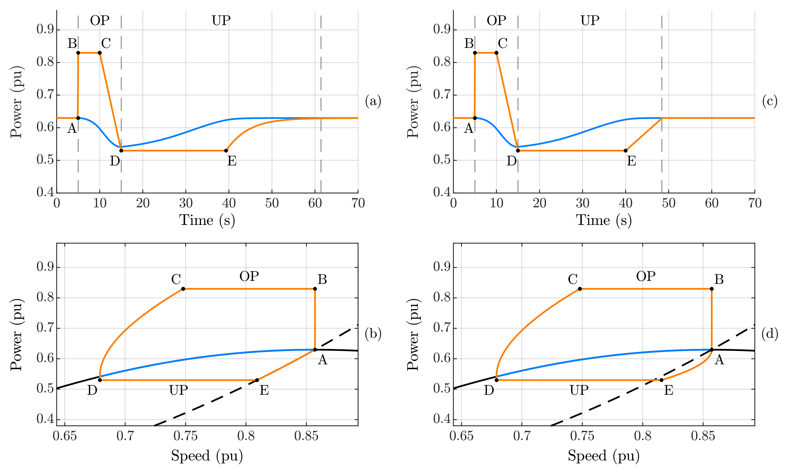
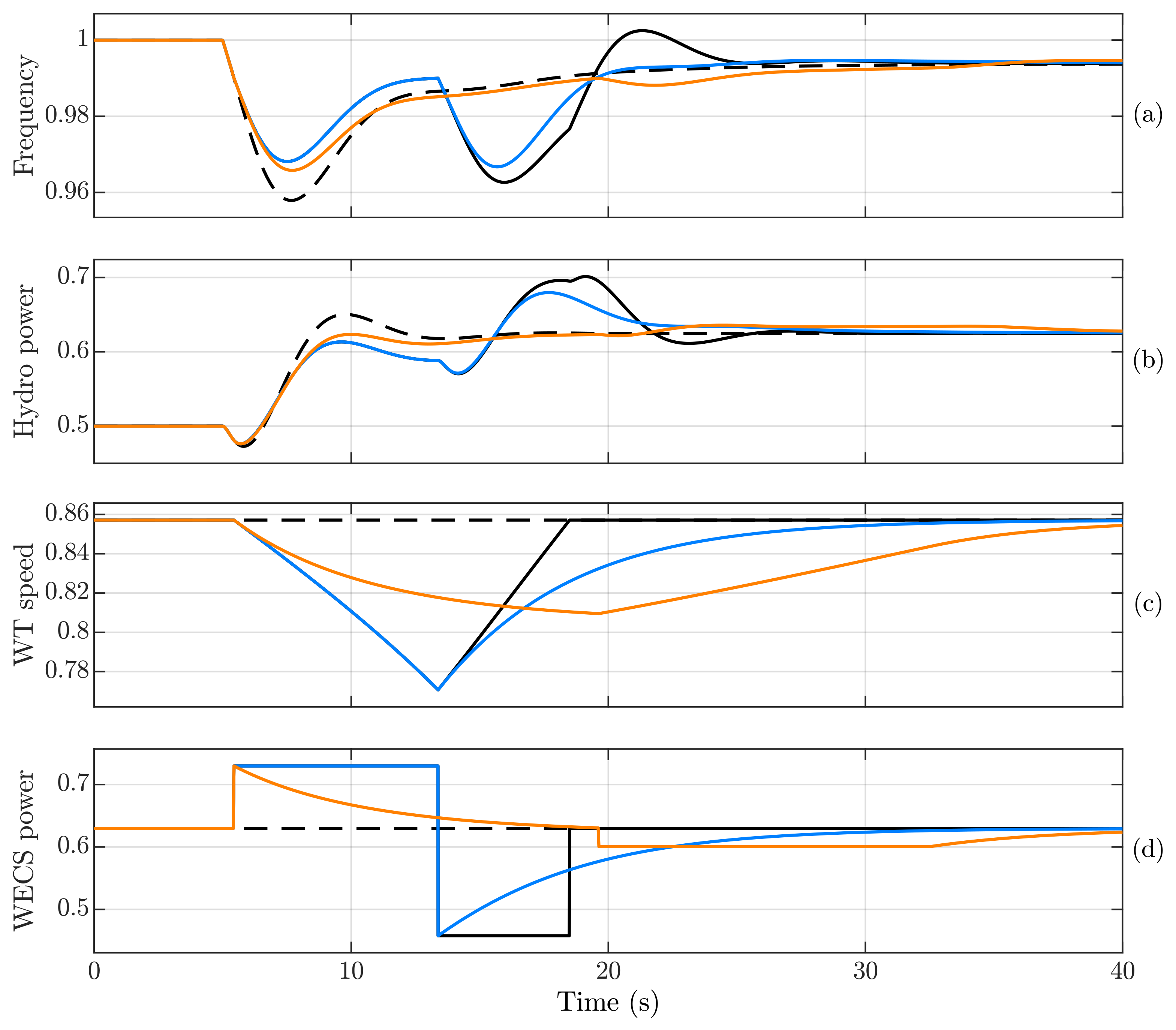
5.1. Fast Power Reserve in Hydro-Dominated Grid

The hydro-based grid exhibits a slow frequency response with a non-minimum phase characteristic [7]. Therefore, the fast power reserve from the wind turbines should be able to assist with transient frequency control after power imbalances. Simulation results comparing various methods are presented in Figure 18. The dashed black curve represents the base case, comprising 75% hydro-generation and 25% installed wind power without frequency control support. Initially, the hydro-generator operates at 0.5 pu, and the wind turbine at 0.63 of its rated power at a constant wind speed in the MPPT region. The rotor speed of the hydro-based generator is equal to the system frequency at 1 pu, and the wind turbine rotor speed is initially about 0.86 pu of its rated value.

At 5 s, a power imbalance of 0.1 pu occurs (based on the system power). The frequency starts to drop, and after a moment, the hydro-generator begins to compensate for the lack of power generation. However, the initial non-minimum phase response momentarily decreases the output power, contributing to the frequency decrease. After about 3 s, the frequency reaches its lowest value—the frequency nadir. Then, the hydro-generator increases its delivered power even more, and the frequency slowly stabilizes over 40 s to a quasi-steady-state value, which is lower than its initial system frequency. Furthermore, the hydro-generator increases its output power to match the power imbalance. In this base case, the wind turbine does not contribute to the frequency control support, so the wind turbine speed and the wind generator output power remain the same during the transient.

The continuous curves show the responses of the wind turbine with some fast power-reserve techniques. The dynamic response is initiated when the frequency drops below 0.99 pu, and the initial power step is 0.1 pu. The black curve represents the method proposed in [46]. When a frequency drop is detected, the generator power reference is increased by 0.1 pu and is maintained until the frequency recovers to 0.99. By this point, the wind turbine has slowed down, and the underproduction stage begins with a constant power reference to recover the turbine speed to the rated value. The transition from overproduction to underproduction modes creates a new power imbalance in the grid, leading to a second-frequency dip, with a frequency nadir even lower than the initial frequency drop. This requires additional power from the hydro-generator. When the wind speed is recovered, there is a third power step reference in the wind generator, which now creates a positive power imbalance. Then, the frequency increases, and the hydro-generator reduces its power to maintain the power balance in the grid.

The blue curve represents the method from [50]. The method is identical to the method from [46] during the overproduction mode, and the curves overlap in Figure 18. During the underproduction mode, the wind generator power reference follows the optimum torque control MPPT technique, allowing the wind turbine to restore its speed gradually. Therefore, the observed second-frequency nadir is higher than the black curve. As the power is slowly restored, there is no third power reference step, so the over-frequency observed in the black curve is not present in the blue curve.

An improvement to mitigate the second-frequency dip is proposed by [52]. During the overproduction mode, 0.1 pu power is added to the MPPT curve. This results in lower output power compared to the black and blue curves, leading to a reduced frequency nadir. However, in the underproduction mode, the power step is much lower (only −0.03 pu), significantly reducing the impact on the second-frequency dip. Therefore, during the restoration stage, the hydropower practically does not need to increase its output, and the frequency response does not exhibit high oscillations. Consequently, a longer time is observed to restore the wind turbine speed.

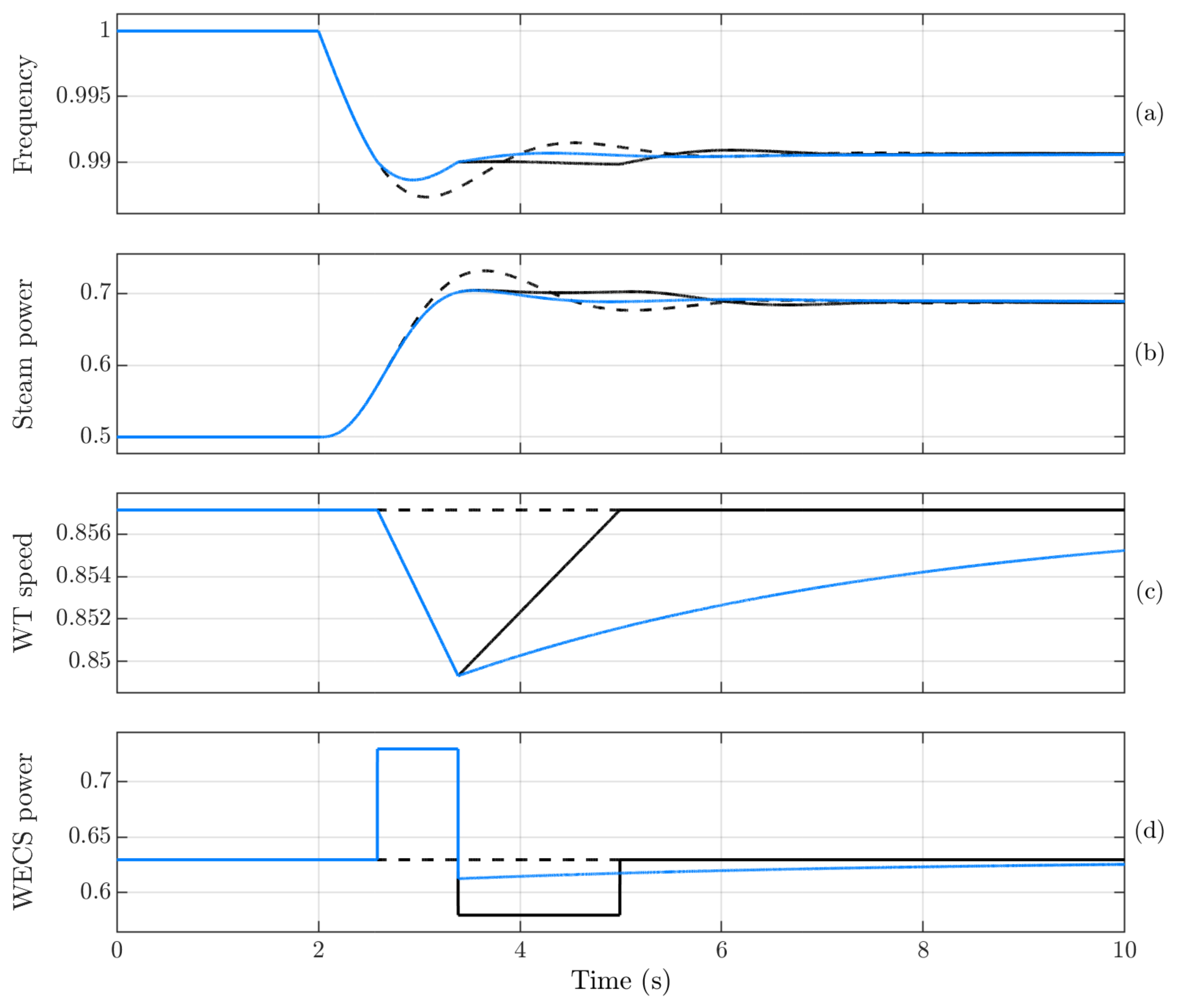
5.2. Fast Power Reserve in Non-Reheat-Steam-Dominated Grid

A second system was evaluated with a composition of $75\%$ steam-based generator and $25\%$ installed wind generation. The steam generator operates initially at 50% of its capacity, and the wind turbine is in the MPPT region with an output power of 0.63 pu. Simulation results are presented in Figure 19. The grid frequency is initially at 1 pu, and the wind turbine speed is at 0.857 pu of its rated value. At 2 s, a power imbalance of 0.15 pu in the grid load occurs, and the frequency starts to drop. The dashed black curve represents the base case without frequency control support. The frequency decreases to a value slightly below 0.99 pu and oscillates until it reaches the quasi-steady-state value. The response from the steam power has an overshoot before settling to the steady-state value.

The continuous curves represent two methods of fast power response. The black curve is the system response when the method from [46] is employed. In this case, the dynamic response is activated when the frequency drops below 0.99 pu. As soon as this condition is verified, the wind generator power reference increases by 0.1 pu and is kept constant until the frequency returns to the threshold value. Then, the underproduction mode starts, and the rotor speed is recovered. It is observed that, as the response from the non-reheat steam turbine is much faster than for a hydro turbine, there is a lower need for wind frequency support. Consequently, the wind turbine rotor speed deviates less, and the power step from overproduction to underproduction mode is smaller than observed in Figure 18. As a result, a second-frequency dip is not observed. A similar conclusion is obtained by observing the blue curve, with the method from [50].

Simulation results in Figure 18 and Figure 19 show that the effectiveness of frequency control support is highly dependent on grid characteristics. For example, a simpler method could be employed in non-reheat steam-based grids due to their faster responses, while a more elaborated method should be used in hydro-based grids to improve the first frequency nadir and avoid subsequent ones.

6. Conclusions

Frequency control support techniques in wind turbines aim to address the issue of low inertia in high non-synchronous renewable grids. Among these techniques, fast power reserve control can be employed to provide a reliable change in delivered power without relying on precise measurements of grid frequency. The primary concept revolves around utilizing the kinetic energy of the wind turbine rotor to deliver transient power without the need for additional energy storage systems or wind turbine deloading. Apart from the initially proposed method, other approaches can be classified based on the function used to generate both over- and underproduction power references.

Speed-dependent methods set a step power reference based on the wind turbine rotor speed. These methods are typically simpler to design and implement since they only require speed measurements. However, these methods often have limited degrees of freedom, and some may exhibit high-power steps and slow recovery periods, leading to second-frequency dips. Time-varying methods use ramp transitions between operating modes. The duration of the transition windows provides additional degrees of freedom for controller design, although they are highly dependent on factors such as the wind turbine model, system type, and the severity of load imbalances. Mechanical power-dependent methods involve estimating the turbine power, which can be achieved through either the turbine model and wind speed measurements or an estimator algorithm based on the system states. If feasible, this information can be used to limit the acceleration and deceleration of the wind turbine, preventing the application of high torque to the shaft and minimizing seconds frequency dips in the grid.

Fast power reserve is a frequency control technique that is independent of the grid frequency, using it solely to initialize the control dynamics. However, certain proposed methods exhibit high power reference steps, potentially causing a second-frequency dip, while others have slow speed restoration, which may degrade control response in the event of consecutive disturbances. Simulation results indicate that these drawbacks are more pronounced in grids with slower characteristics, such as hydro-based grids, where more effective methods should be considered. In fast-controlled grids, such as those using non-reheat steam turbines, the side effects of fast power reserves are less prominent. As a result, a simple method is often sufficient to provide fast power reserve safely without drawbacks, improving frequency nadir and reducing the absolute rate of change of frequency.

The various methods for fast power reserve underscore the importance of carefully designing the wind energy conversion system in alignment with the characteristics of the grid. Current research in this field emphasizes determining suitable power reference trajectories with the goal of providing an adequate amount of additional power in case of under-frequency events without causing second-frequency dips during the transient period. Additionally, researchers focus on parameter optimization, which can vary based on the characteristics of the conventional generators, the percentage of wind penetration, wind speed, and expected power imbalances. The ongoing challenge lies in balancing the contribution to frequency regulation while minimizing side effects in the wind energy conversion system, such as torque overload and energy losses.

References

1. Steg, L.; Shwom, R.; Dietz, T. What Drives Energy Consumers?: Engaging People in a Sustainable Energy Transition. IEEE Power Energy Mag. 2018, 16, 20–28. [Google Scholar] [CrossRef]
2. Ipakchi, A.; Albuyeh, F. Grid of the future. IEEE Power Energy Mag. 2009, 7, 52–62. [Google Scholar] [CrossRef]
3. Rodriguez, J.; Blaabjerg, F.; Kazmierkowski, M.P. Energy Transition Technology: The Role of Power Electronics. Proc. IEEE 2023, 111, 329–334. [Google Scholar] [CrossRef]
4. Peyghami, S.; Sahoo, S.; Wang, H.; Wang, X.; Blaabjerg, F. The Role of Power Electronics in Modern Energy System Integration. Found. Trends Electr. Energy Syst. 2022, 5, 1–74. [Google Scholar] [CrossRef]
5. Perez-Arriaga, I.J. The Transmission of the Future: The Impact of Distributed Energy Resources on the Network. IEEE Power Energy Mag. 2016, 14, 41–53. [Google Scholar] [CrossRef]
6. Fortuna, L.; Buscarino, A. Sustainable Energy Systems. Energies 2022, 15, 9227. [Google Scholar] [CrossRef]
7. Kundur, P.S.; Malik, O.P. Power System Stability and Control; McGraw-Hill Education: New York, NY, USA, 2022. [Google Scholar]
8. Tielens, P.; Van Hertem, D. The relevance of inertia in power systems. Renew. Sustain. Energy Rev. 2016, 55, 999–1009. [Google Scholar] [CrossRef]
9. Carrasco, J.M.; Franquelo, L.G.; Bialasiewicz, J.T.; Galvan, E.; Guisado, R.C.P.; Prats, M.A.M.; Leon, J.I.; Moreno-Alfonso, N. Power-electronic systems for the grid integration of renewable energy sources: A survey. IEEE Trans. Ind. Electron. 2006, 53, 1002–1016. [Google Scholar] [CrossRef]
10. Fang, J.; Li, H.; Tang, Y.; Blaabjerg, F. On the Inertia of Future More-Electronics Power Systems. IEEE J. Emerg. Sel. Top. Power Electron. 2019, 7, 2130–2146. [Google Scholar] [CrossRef]
11. Kundur, P.; Paserba, J.; Ajjarapu, V.; Andersson, G.; Bose, A.; Canizares, C.; Hatziargyriou, N.; Hill, D.; Stankovic, A.; Taylor, C.; et al. Definition and classification of power system stability. IEEE Trans. Power Syst. 2004, 19, 1387–1401. [Google Scholar] [CrossRef]
12. Bevrani, H.; François, B.; Ise, T. Microgrid Dynamics and Control; John Wiley & Sons: Hoboken, NJ, USA, 2017. [Google Scholar]
13. Meegahapola, L.; Sguarezi, A.; Bryant, J.S.; Gu, M.; Conde, D.E.R.; Cunha, R.B.A. Power system stability with power-electronic converter interfaced renewable power generation: Present issues and future trends. Energies 2020, 13, 3441. [Google Scholar] [CrossRef]
14. Deng, X.; Mo, R.; Wang, P.; Chen, J.; Nan, D.; Liu, M. Review of RoCoF Estimation Techniques for Low-Inertia Power Systems. Energies 2023, 16, 3708. [Google Scholar] [CrossRef]
15. Yan, R.; Al-Masood, N.; Saha, T.K.; Bai, F.; Gu, H. The anatomy of the 2016 South Australia blackout: A catastrophic event in a high renewable network. IEEE Trans. Power Syst. 2018, 33, 5374–5388. [Google Scholar] [CrossRef]
16. NERC. 900 MW Fault Induced Solar Photovoltaic Resource Interruption Disturbance Report; Joined NERC and WECC Staff Report; NERC: Atlanta, GA, USA, 2018. [Google Scholar]
17. Zhang, G.; Zhong, H.; Tan, Z.; Cheng, T.; Xia, Q.; Kang, C. Texas electric power crisis of 2021 warns of a new blackout mechanism. CSEE J. Power Energy Syst. 2022, 8, 1–9. [Google Scholar] [CrossRef]
18. Li, L.; Zhu, D.; Zou, X.; Hu, J.; Kang, Y.; Guerrero, J.M. Review of frequency regulation requirements for wind power plants in international grid codes. Renew. Sustain. Energy Rev. 2023, 187, 113731. [Google Scholar] [CrossRef]
19. Williams, R.; Zhao, F.; Lee, J. GWEC—Global Offshore Wind Report 2022. Glob. Wind Energy Counc. 2022, 29, 10–12. [Google Scholar]
20. Yaramasu, V.; Wu, B.; Sen, P.C.; Kouro, S.; Narimani, M. High-power wind energy conversion systems: State-of-the-art and emerging technologies. Proc. IEEE 2015, 103, 740–788. [Google Scholar] [CrossRef]
21. Anaya-Lara, O.; Tande, J.O.; Uhlen, K.; Merz, K. Offshore Wind Energy Technology; John Wiley & Sons: Hoboken, NJ, USA, 2018. [Google Scholar]
22. Teodorescu, R.; Liserre, M.; Rodriguez, P. Grid Converters for Photovoltaic and Wind Power Systems; John Wiley & Sons: Hoboken, NJ, USA, 2011. [Google Scholar]
23. Yaramasu, V.; Wu, B. Model Predictive Control of Wind Energy Conversion Systems; John Wiley & Sons: Hoboken, NJ, USA, 2016. [Google Scholar]
24. Golestan, S.; Guerrero, J.M.; Vasquez, J.C. Three-Phase PLLs: A Review of Recent Advances. IEEE Trans. Power Electron. 2017, 32, 1894–1907. [Google Scholar] [CrossRef]
25. Margaris, I.D.; Papathanassiou, S.A.; Hatziargyriou, N.D.; Hansen, A.D.; Sorensen, P. Frequency Control in Autonomous Power Systems with High Wind Power Penetration. IEEE Trans. Sustain. Energy 2012, 3, 189–199. [Google Scholar] [CrossRef]
26. Tamrakar, U.; Shrestha, D.; Maharjan, M.; Bhattarai, B.P.; Hansen, T.M.; Tonkoski, R. Virtual inertia: Current trends and future directions. Appl. Sci. 2017, 7, 654. [Google Scholar] [CrossRef]
27. Arani, M.F.M.; Mohamed, Y.A.R.I. Analysis and mitigation of undesirable impacts of implementing frequency support controllers in wind power generation. IEEE Trans. Energy Convers. 2016, 31, 174–186. [Google Scholar] [CrossRef]
28. Fini, M.H.; Golshan, M.E.H.; Martí, J.R.; Ketabi, A. Determining the Required Frequency Control Reserve and Capacity and Location of Synchronous and Virtual Inertial Resources. IEEE Trans. Sustain. Energy 2022, 14, 27–38. [Google Scholar] [CrossRef]
29. Fernández-Bustamante, P.; Barambones, O.; Calvo, I.; Napole, C.; Derbeli, M. Provision of frequency response from wind farms: A review. Energies 2021, 14, 6689. [Google Scholar] [CrossRef]
30. Dreidy, M.; Mokhlis, H.; Mekhilef, S. Inertia response and frequency control techniques for renewable energy sources: A review. Renew. Sustain. Energy Rev. 2017, 69, 144–155. [Google Scholar] [CrossRef]
31. Cheng, Y.; Azizipanah-Abarghooee, R.; Azizi, S.; Ding, L.; Terzija, V. Smart frequency control in low inertia energy systems based on frequency response techniques: A review. Appl. Energy 2020, 279, 115798. [Google Scholar] [CrossRef]
32. Wu, Z.; Gao, W.; Gao, T.; Yan, W.; Zhang, H.; Yan, S.; Wang, X. State-of-the-art review on frequency response of wind power plants in power systems. J. Mod. Power Syst. Clean Energy 2018, 6, 1–16. [Google Scholar] [CrossRef]
33. Sonkar, P.; Rahi, O. Contribution of wind power plants in grid frequency regulation: Current perspective and future challenges. Wind Eng. 2021, 45, 442–456. [Google Scholar] [CrossRef]
34. Bhowon, A.; Abo-Al-Ez, K.M.; Adonis, M. Variable-Speed Wind Turbines for Grid Frequency Support: A Systematic Literature Review. Mathematics 2022, 10, 3586. [Google Scholar] [CrossRef]
35. Avon, G.; Bucolo, M.; Buscarino, A.; Fortuna, L. Sensing Frequency Drifts: A Lookup Table Approach. IEEE Access 2022, 10, 96249–96259. [Google Scholar] [CrossRef]
36. Wu, B.; Lang, Y.; Zargari, N.; Kouro, S. Power Conversion and Control of Wind Energy Systems; John Wiley & Sons: Hoboken, NJ, USA, 2011; Volume 76. [Google Scholar]
37. Chen, Z.; Guerrero, J.M.; Blaabjerg, F. A review of the state of the art of power electronics for wind turbines. IEEE Trans. Power Electron. 2009, 24, 1859–1875. [Google Scholar] [CrossRef]
38. Taherian-Fard, E.; Sahebi, R.; Niknam, T.; Izadian, A.; Shasadeghi, M. Wind turbine drivetrain technologies. IEEE Trans. Ind. Appl. 2020, 56, 1729–1741. [Google Scholar] [CrossRef]
39. Polinder, H.; Pijl, F.F.V.D.; Vilder, G.J.D.; Tavner, P.J. Comparison of direct-drive and geared generator concepts for wind turbines. IEEE Trans. Energy Convers. 2006, 21, 725–733. [Google Scholar] [CrossRef]
40. Hau, E. Wind Turbines: Fundamentals, Technologies, Application, Economics; Springer Science & Business Media: Berlin/Heidelberg, Germany, 2013. [Google Scholar]
41. Carpintero-Renteria, M.; Santos-Martin, D.; Lent, A.; Ramos, C. Wind turbine power coefficient models based on neural networks and polynomial fitting. IET Renew. Power Gener. 2020, 14, 1841–1849. [Google Scholar] [CrossRef]
42. Gaertner, E.; Rinker, J.; Sethuraman, L.; Zahle, F.; Anderson, B.; Barter, G.; Abbas, N.; Meng, F.; Bortolotti, P.; Skrzypinski, W.; et al. Definition of the IEA Wind 15-Megawatt Offshore Reference Wind Turbine Technical Report; National Renewable Energy Laboratory: Golden, CO, USA, 2020. [Google Scholar]
43. Abbas, N.J.; Zalkind, D.S.; Pao, L.; Wright, A. A reference open-source controller for fixed and floating offshore wind turbines. Wind Energy Sci. 2022, 7, 53–73. [Google Scholar] [CrossRef]
44. Kumar, D.; Chatterjee, K. A review of conventional and advanced MPPT algorithms for wind energy systems. Renew. Sustain. Energy Rev. 2016, 55, 957–970. [Google Scholar] [CrossRef]
45. Eriksson, R.; Modig, N.; Elkington, K. Synthetic inertia versus fast frequency response: A definition. Inst. Eng. Technol. 2018, 12, 507–514. [Google Scholar] [CrossRef]
46. Ullah, N.R.; Thiringer, T.; Karlsson, D. Temporary primary frequency control support by variable speed wind turbines—Potential and applications. IEEE Trans. Power Syst. 2008, 23, 601–612. [Google Scholar] [CrossRef]
47. Keung, P.K.; Li, P.; Banakar, H.; Ooi, B.T. Kinetic Energy of Wind-Turbine Generators for System Frequency Support. IEEE Trans. Power Syst. 2009, 24, 279–287. [Google Scholar] [CrossRef]
48. Tarnowski, G.C.; Kjar, P.C.; Sorensen, P.E.; Ostergaard, J. Variable speed wind turbines capability for temporary over-production. In Proceedings of the 2009 IEEE Power & Energy Society General Meeting, Calgary, AB, Canada, 26–30 July 2009; pp. 1–7. [Google Scholar] [CrossRef]
49. El Itani, S.; Annakkage, U.D.; Joos, G. Short-term frequency support utilizing inertial response of DFIG wind turbines. In Proceedings of the 2011 IEEE Power and Energy Society General Meeting, Detroit, MI, USA, 24–28 July 2011; pp. 1–8. [Google Scholar] [CrossRef]
50. Hansen, A.D.; Altin, M.; Margaris, I.D.; Iov, F.; Tarnowski, G.C. Analysis of the short-term overproduction capability of variable speed wind turbines. Renew. Energy 2014, 68, 326–336. [Google Scholar] [CrossRef]
51. Hafiz, F.; Abdennour, A. Optimal use of kinetic energy for the inertial support from variable speed wind turbines. Renew. Energy 2015, 80, 629–643. [Google Scholar] [CrossRef]
52. Kang, M.; Muljadi, E.; Hur, K.; Kang, Y.C. Stable Adaptive Inertial Control of a Doubly-Fed Induction Generator. IEEE Trans. Smart Grid 2016, 7, 2971–2979. [Google Scholar] [CrossRef]
53. Kang, M.; Kim, K.; Muljadi, E.; Park, J.W.; Kang, Y.C. Frequency Control Support of a Doubly-Fed Induction Generator Based on the Torque Limit. IEEE Trans. Power Syst. 2016, 31, 4575–4583. [Google Scholar] [CrossRef]
54. Xu, G.; Xu, L. Improved use of WT kinetic energy for system frequency support. IET Renew. Power Gener. 2017, 11, 1094–1100. [Google Scholar] [CrossRef]
55. Yang, D.; Kang, M.; Muljadi, E.; Gao, W.; Hong, J.; Choi, J.; Kang, Y.C. Short-Term Frequency Response of a DFIG-Based Wind Turbine Generator for Rapid Frequency Stabilization. Energies 2017, 10, 1863. [Google Scholar] [CrossRef]
56. Wang, S.; Tomsovic, K. Quantitative Control Approach for Wind Turbine Generators to Provide Fast Frequency Response with Guarantee of Rotor Security. IEEE Power Energy 2018, 85, 1–5. [Google Scholar] [CrossRef]
57. Yang, D.; Kim, J.; Kang, Y.C.; Muljadi, E.; Zhang, N.; Hong, J.; Song, S.H.; Zheng, T. Temporary Frequency Support of a DFIG for High Wind Power Penetration. IEEE Trans. Power Syst. 2018, 33, 3428–3437. [Google Scholar] [CrossRef]
58. Liu, K.; Qu, Y.; Kim, H.M.; Song, H. Avoiding Frequency Second Dip in Power Unreserved Control During Wind Power Rotational Speed Recovery. IEEE Trans. Power Syst. 2018, 33, 3097–3106. [Google Scholar] [CrossRef]
59. Kheshti, M.; Ding, L.; Nayeripour, M.; Wang, X.; Terzija, V. Active power support of wind turbines for grid frequency events using a reliable power reference scheme. Renew. Energy 2019, 139, 1241–1254. [Google Scholar] [CrossRef]
60. Yang, D.; Gao, H.C.; Zhang, L.; Zheng, T.; Hua, L.; Zhang, X. Short-term frequency support of a doubly-fed induction generator based on an adaptive power reference function. Int. J. Electr. Power Energy Syst. 2020, 119, 105955. [Google Scholar] [CrossRef]
61. Kheshti, M.; Lin, S.; Zhao, X.; Ding, L.; Yin, M.; Terzija, V. Gaussian Distribution-Based Inertial Control of Wind Turbine Generators for Fast Frequency Response in Low Inertia Systems. IEEE Trans. Sustain. Energy 2022, 13, 1641–1653. [Google Scholar] [CrossRef]
62. European Network of Transmission System Operators for Electricity. Inertia and Rate of Change of Frequency (RoCoF); European Network of Transmission System Operators for Electricity: Brussels, Belgium, 2020. [Google Scholar]
63. Chen, L.; Lu, Z.; Min, Y.; Yu, R.; Liu, B.; Chen, Q. Analysis of power system frequency oscillations with intentional governor deadbands using describing functions. Int. J. Electr. Power Energy Syst. 2019, 111, 390–397. [Google Scholar] [CrossRef]
64. Zhang, Z.; Du, E.; Teng, F.; Zhang, N.; Kang, C. Modeling Frequency Dynamics in Unit Commitment with a High Share of Renewable Energy. IEEE Trans. Power Syst. 2020, 35, 4383–4395. [Google Scholar] [CrossRef]
65. Lokay, H.E.; Burtnyk, V. Application of Underfrequency Relays for Automatic Load Shedding. IEEE Trans. Power Appar. Syst. 1968, 87, 776–783. [Google Scholar] [CrossRef]
Figure 1. Simplified diagram depicting the most common WECS configurations: (a) Type III, featuring partial power processing, and (b) Type IV, employing full-scale power processing.
Energies 17 00451 g001
Figure 2. Simplified control scheme for a Type-IV WECS, comprising a wind turbine, a permanent magnet synchronous generator, and a back-to-back converter. The control system includes pitch angle control, maximum-power point tracking, fast power reserve, and generator-side current control.
Energies 17 00451 g002
Figure 3. Power coefficient as a function of the tip–speed ratio for various blade pitch angles. Black curve: β = 0 ° ; blue curve: β = 10 ° ; and orange curve: β = 20 ° .
Energies 17 00451 g003
Figure 4. Steady-state wind turbine power curve and operating regions as a function of the wind speed. Region 1: Turbine is turned off due to low wind speed; Region 1.5: operation at minimum rotor speed; Region 2: operation with maximum-power point tracking; Region 3: operation with limited power; and Region 4: turbine is turned off due to high wind speed.
Energies 17 00451 g004
Figure 5. Implementation of the control scheme proposed by [46]. Mode 0: MPPT; Mode 1: Overproduction; Mode 2: Underproduction.
Energies 17 00451 g005
Figure 6. Fast power-reserve dynamics utilizing the strategy proposed by [46]. Generator power (orange) and wind turbine power (blue) are depicted as functions of (a) time and (b) rotor speed. Point A: initial state; Points B, C: overproduction mode; Points D, E: underproduction mode; Point F: end state.
Energies 17 00451 g006
Figure 7. Contour lines illustrating the maximum overproduction duration (5, 10, 20, and 40 s) as a function of overproduction power (pu) and wind speed (m/s).
Energies 17 00451 g007
Figure 8. Contour lines illustrating the recovery time (5 and 10 s) in the MPPT region from the minimum rotating speed, based on the underproduction power step (pu) and wind speed (m/s).
Energies 17 00451 g008
Figure 9. Control scheme of the implemented method based on [50]. Mode 0: MPPT and Underproduction; Mode 1: Overproduction.
Energies 17 00451 g009
Figure 10. Fast power-reserve dynamics based on the strategy of [50]. Generator power (orange) and wind turbine power (blue) as functions of (a) time and (b) rotor speed. Point A: initial state; Points B, C: overproduction mode; Point D: underproduction mode.
Energies 17 00451 g010
Figure 11. Control scheme for the implemented methods based on: (a) [52], with a constant power added to the MPPT reference during overproduction mode, and (b) [53], with an overproduction power limited to the maximum torque and decaying with rotor speed.
Energies 17 00451 g011
Figure 12. Fast power-reserve dynamics based on the strategy proposed in [52] (a,b) and [53] (c,d). The figure depicts the generator power (in orange) and wind turbine power (in blue) as functions of time (a,c) and rotor speed (b,d). The dashed line in (b,d) represents the MPPT power reference, while the dotted line in (d) indicates the power reference resulting in the rated torque. Point A: initial state; Points B, C: overproduction (OP) mode; Points D, E: underproduction (UP) mode.
Energies 17 00451 g012
Figure 13. Fast power-reserve dynamics based on the strategies of [58], implemented as the power reference. Generator power is represented in orange, and wind turbine power in blue, both as functions of rotor speed. The dashed line corresponds to the MPPT power reference. The figure displays the (a) square, (b) oval, (c) index, and (d) linear methods. Point A: initial state; Points B, C overproduction mode; Points D, E: underproduction mode.
Energies 17 00451 g013
Figure 14. Fast power-reserve dynamics based on the strategies proposed by [49] (a,b) and [51] (c,d). Generator power is depicted in orange, and wind turbine power in blue, as functions of time (a,c) and rotor speed (b,d). The dashed line represents the MPPT power reference. Point A: initial state; points B, C overproduction (OP) mode; Points D, E: underproduction (UP) mode.
Energies 17 00451 g014
Figure 15. Fast power-reserve dynamics based on the strategy proposed by [48]. Generator power is represented in orange, and wind turbine power in blue, as functions of (a) time and (b) rotor speed. Point A: initial state; Points B, C: overproduction (OP) mode; Points D, E: underproduction (UP) mode; Point F: end state.
Energies 17 00451 g015
Figure 16. Fast power-reserve dynamics based on the strategies proposed by [54]. Generator power is depicted in orange, and wind turbine power in blue, as functions of time (a,c) and rotor speed (b,d) for the first (a,b) and second (c,d) strategies. Point A: initial state; Points B, C overproduction (OP) mode; Points D, E: underproduction (UP) mode; Point F: end state.
Energies 17 00451 g016
Figure 17. Typical frequency response following a power imbalance in the system, illustrating the dynamics of system inertia and frequency primary and secondary controls. t i —Initial point; t n —Time duration to reach frequency nadir ( f n ); f s s —Quasi-steady-state frequency after primary control; f i —Initial and steady-state frequency. Adapted from [10].
Energies 17 00451 g017
Figure 18. Simulation results in per unit for a wind turbine in the MPPT region with fast power-reserve control following a grid power imbalance of −0.1 pu at 5 s in a hydro-generation-dominated grid. The graphics show: (a) Grid frequency, (b) hydropower, (c) wind turbine speed, and (d) WECS output power. The dashed black curve represents the base case without frequency response, while the solid black curve corresponds to the method from [46], the blue curve to the method from [50], and the orange curve to the method from [52].
Energies 17 00451 g018
Figure 19. Simulation results per unit for a wind turbine in the MPPT region with fast power reserve control following a grid power imbalance of −0.15 pu at 2 s in a non-reheat steam generation-dominated grid. The graphs illustrate: (a) Grid frequency, (b) steam power, (c) wind turbine speed, and (d) WECS output power. The dashed black curve represents the base case without frequency response, while the solid black curve corresponds to the method from [46], and the blue curve represents the method from [50].
Energies 17 00451 g019