Abstract
Wind energy, as a key link in renewable energy, has seen its penetration in the power grid increase in recent years. In this context, accurate and reliable short-term wind power prediction is particularly important for the real-time scheduling and operation of power systems. However, many deep learning-based methods rely on the relationship between wind speed and wind power to build a prediction model. These methods tend to consider only the temporal features and ignore the spatial and frequency domain features of the wind power variables, resulting in poor prediction accuracy. In addition to this, existing power forecasts for wind farms are often based on the wind farm level, without considering the impact of individual turbines on the wind power forecast. Therefore, this paper proposes a wind power prediction model based on multi-feature domain learning (MFDnet). Firstly, the model captures the similarity between turbines using the latitude, longitude and wind speed of the turbines, and constructs a turbine group with similar features as input based on the nearest neighbor algorithm. On this basis, the Seq2Seq framework is utilized to achieve weighted fusion with temporal and spatial features in multi-feature domains through high-frequency feature extraction by DWT. Finally, the validity of the model is verified with data from a wind farm in the U.S. The results show that the overall performance of the model outperforms other wind farm power prediction algorithms, and reduces MAE by 25.5% and RMSE by 20.6% compared to the baseline persistence model in predicting the next hour of wind power.
1. Introduction
The world is facing challenges such as climate change, resource shortages, and environmental pollution. Gradually replacing traditional fossil fuel power generation with renewable energy has become a development trend [], and sustainable development has become the guiding principle of the global energy transformation []. In this transformation, wind energy, as a clean and renewable energy source, plays a vital role. The popularization and utilization of wind energy can help reduce environmental pollution and carbon emissions and promote sustainable development. With the advancement of technology and industry, countries are actively developing and utilizing wind energy and integrating wind power into the power grid to promote the development of clean energy. However, the volatility and stochastic nature of wind power pose significant challenges for the power system when it is incorporated into the grid. Therefore, accurate short-term wind power prediction is particularly important. Such predictions not only help improve grid dispatching efficiency and reduce operating costs but also enhance the security, reliability, and controllability of the system [,,,].
According to the time scale, researchers categorize wind power prediction into ultra-short-term prediction (less than 30 min), short-term prediction (30 min to 6 h), medium-term prediction (6 h to 1 day), and long-term prediction (1 day to 7 days). These types of predictions play different roles in the actual operation of the power system. Short-term prediction not only affects real-time dispatch but also has an important impact on power generation plans. This is because it can guide the formulation of power generation plans several hours in advance, enabling more efficient utilization of generation resources. Accurate short-term forecasts ensure stable grid operation and rational allocation of generation resources, which is of profound significance for achieving efficient operation and reliable power supply for the power system. Therefore, accurate short-term forecasting has become the focus of researchers’ attention in recent years.
In recent decades, there have been three main categories of wind power prediction (WPP) methods: physical methods, statistical methods, and artificial intelligence methods.
The physical approach describes the physical relationship between weather conditions, topography, wind speed, and wind turbine power, using the resulting numerical weather prediction (NWP) as input to the wind power prediction model without the need for historical wind power data. Statistical models that analyze the time series of historical data can directly describe the link between wind speed and wind power generation as predicted by the NWP without taking into account the physical characteristics of the generation system. For example, Christos Stathopoulos et al. explored the problem of wind power prediction through numerical and statistical prediction models and verified that accurate wind power prediction can be achieved under the condition of reliable local environmental data []. Michael Milligan et al. developed a class of autoregressive moving average (ARMA) models applied to wind speed and wind output []. Xiaosheng Peng et al. proposed a data mining-based regional power prediction method to optimize the input parameters, which is highly superior to traditional prediction methods []. P. Lakshmi Deepak proposed an improved linear regression algorithm that overcomes the limitations of ridge regression, achieving better wind power forecasting [].
The AI method makes future wind power predictions by learning the relationship between past weather conditions and the power output generated from past time series. Unlike statistical methods based on explicit statistical analysis, the AI method excels in characterizing the nonlinear and highly complex relationships between the input data (NWP forecasts and output power). Thus, it can achieve better prediction results in scenarios involving short-term wind power prediction. For example, Jianwu Zeng et al. proposed a short-term WPP model based on support vector machines to predict the wind speed. Then they utilize the power–wind speed characteristics of the wind turbine generator to predict wind power, which provides better prediction accuracy for both ultra-short-term and short-term WPPs []. Guoqing An et al. proposed an Adaboost algorithm combined with a particle swarm optimization extreme learning machine (PSO-ELM) in conjunction with a wind power prediction model []. Bowen Zhou et al. studied weather forecast data as one of the inputs to the long short-term memory (LSTM) network model to realize the on-site prediction of wind farm power []. Jie Hao et al. proposed an improved random forest short-term prediction model based on hierarchical output power, which adopts Poisson resampling instead of random forest’s bootstrap to improve the training speed of the random forest algorithm []. Weisi Deng et al. proposed a short-term WPP method for windy weather based on wind speed interval segmentation and TimeGAN, which improves the accuracy of short-term wind power prediction []. Md Alamgir Hossain et al. developed a prediction modeling framework consisting of LSTM, complete ensemble empirical mode decomposition with adaptive noise (CEEMDAN), and monarch butterfly optimization (MBO) algorithms, which has low computation time and satisfactory performance []. Wei Fan and colleagues propose an A-GRU-S2S model based on the sequence-to-sequence GRU architecture, which eliminates the model’s dependency on temporal distance information, thereby effectively predicting ultra-short-term power output of wind farms []. Jiaqiu Hu and colleagues have introduced a forecasting model based on Neural Prophet, which enhances the accuracy of wind power prediction and the integration capability of renewable energy during cold wave conditions []. Nanyang Zhu et al. proposed GGNet, a granularity-based GNN with better performance than the state-of-the-art (SoTA) method []. The above studies have shown that prediction models based on artificial intelligence methods can achieve high-resolution wind power prediction. However, most of them still suffer from several drawbacks, such as:
- Most of them rely on the relationship between wind speed and wind power to build the prediction models, and lack consideration for additional features such as time features, spatial features, and so on.
- There is a lack of consideration of individual turbines when measuring wind farm power.
In summary, a short-term wind power prediction model based on multi-feature domain learning (MFDnet) is proposed in this paper. The method leverages the complementary characteristics of temporal, spatial correlation, and frequency domain information, integrates wind speed latitude and longitude data from different turbines, along with time information, utilizes the high-pass filtering characteristics of wavelet transform to capture the high-speed changing components of the signal, and improves the model’s sensitivity to the short-term signal transformation. Additionally, a similarity matrix is introduced to design a spatial similarity nearest neighbor algorithm (SSNN) to reduce the dependence of wind power prediction on wind speed. The main contributions of this paper are:
- The idea of integrating multiple feature domains is introduced into wind power prediction, which improves the prediction accuracy through the complementary characteristics of temporal, spatial and frequency domains.
- A SSNN is proposed to obtain correlation information between multiple turbines using historical latitude and longitude information and historical wind speed information from different turbines, thus reducing the uncertainty transfer caused by previous wind speed dependent forecasts.
- In the selected dataset, we propose a new wind power forecasting model that performs individual wind power predictions for each turbine in a wind farm and then combines the predictions for an overall wind farm forecast. Compared to other competing algorithms, it demonstrates superior performance. Specifically, the model outperforms other wind farm power prediction algorithms in overall performance and reduces the MAE by 25.5% and RMSE by 20.6% when predicting the wind power for the next 1 h compared to the baseline persistence model.
2. Data Processing
The dataset utilized in this paper is sourced from [], originating from a flat terrain inland wind farm located in the United States. It encompasses hourly wind speeds and wind power data for 200 turbines randomly selected over the period of 2010 to 2011. The dataset covers the time period from 9 January 2010 to 31 August 2011, with a temporal resolution of 60 min. The overall ratio of anomalous and missing data is less than 2%. The statistical summary of the dataset is presented in Table 1, which includes measures such as mean, standard deviation (Std), minimum value (Min), and maximum value (Max).

Table 1.
The statistical summary of the dataset.
Additionally, the dataset incorporates hourly wind speed and direction measurements from three meteorological masts. Notably, it includes the relative coordinates (latitude and longitude) of the 200 turbines. It is important to note that due to the confidentiality surrounding the exact location of the wind farm, the provided dataset contains relative positions of the real data with an added constant. However, the layout remains consistent with the actual arrangement. Therefore, this dataset has no effect on the prediction accuracy of the algorithm proposed in this paper [].
2.1. Feature Selection
Feature selection plays a pivotal role in enhancing the accuracy and reliability of wind power prediction models. In this section, we conduct various correlation analyses to uncover the inherent relationships within the data in our dataset, laying the groundwork for our feature selection process. Given the paramount importance of meteorological factors in wind power prediction, our initial focus is on examining the correlation between wind speed and wind power.
To quantify this correlation, we employ the Pearson correlation coefficient, a widely-used statistical metric for assessing the strength and direction of linear relationships between two variables. Ranging from −1 to 1, the Pearson correlation coefficient provides insights into how changes in one variable correspond to changes in another. A positive correlation coefficient indicates a positive relationship, where an increase in one variable corresponds to an increase in the other. Conversely, a negative correlation coefficient signifies an inverse relationship, with an increase in one variable associated with a decrease in the other. A correlation coefficient near 0 suggests little to no linear relationship between the variables.
The formula for calculating the Pearson correlation coefficient is as follows:
where, , are the wind power and wind speed at the moment, and denote the mean value of wind speed and wind power, respectively, and n is the length of time (h).
Specifically, we initially screened numbers from 1 to 200 with an incremental factor of 10. This resulted in a series of turbines numbered 1, 10, 20, 30,..., 190, and 200, totaling 21 turbines. The wind power and wind speed of these 21 turbines were tested for Pearson similarity at the same moment. The final results are presented in Figure 1. It can be observed that the correlation coefficients between different turbines consistently range from 0.90 to 1.00. This indicates a strong correlation between wind speed and wind power in this dataset, justifying the consideration of wind speed as a correlation factor for wind power prediction.
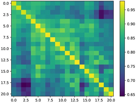
Figure 1.
Correlation between wind speed and wind power.
Additionally, it is essential to assess the temporal autocorrelation of the wind power and the wind speed series. Figure 2 illustrates the Pearson autocorrelation coefficients of the wind power series with different lags. Figure 3 illustrates the Pearson autocorrelation coefficients of the wind power series with different lags.
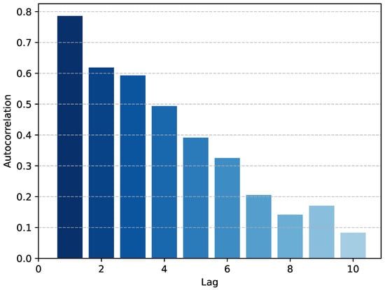
Figure 2.
Autocorrelation of wind power at different lags.
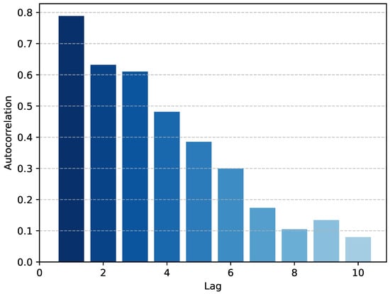
Figure 3.
Autocorrelation of wind speed at different lags.
It can be seen that the autocorrelation coefficient decreases sharply at the first few lags, and when the lag is not more than 6 h, the autocorrelation coefficient is greater than 0.3. Therefore, this indicates a stronger autocorrelation among the wind data during these early time points, as well as wind speed data, and we can use the wind speed as the characterization input in the prediction of short-term wind power.
Based on the aforementioned analysis, wind speed, time, latitude, and longitude have been selected as inputs for the prediction task in this study. The wind speeds represent a key factor for modeling wind power prediction, while the latter two introduce the concepts of temporal and spatial features, respectively.
In this paper, the timestamp is formatted in reserved hours, enabling its utilization as a feature input for the model. As demonstrated earlier, wind speed and wind power data tend to exhibit temporal correlation; that is, wind speed and wind power at the current time may be correlated with data from previous time periods. By incorporating time as a feature into the model, this temporal correlation can be more effectively considered, thereby enhancing the prediction accuracy of the model.
Furthermore, this study utilizes latitude and longitude as spatial feature inputs, enabling the model to capture the correlations among turbine spatial nodes [].
Therefore, in the subsequent chapter, we propose a novel approach to address this issue.
2.2. Data Preprocessing
In order to ensure the quality of the raw data and the accuracy of the prediction, the input wind power data and wind speed data are firstly processed with missing values, and the linear interpolation method is used in this paper, whose formula can be expressed as:
where , are timestamps and , are the corresponding wind power or wind speed magnitudes.
Additionally, to mitigate the impact of differing scales and distributions of features [], this paper employs Min-Max normalization to scale the wind power and wind speed to a range between 0 and 1, which is shown in Equation (3). The outcome of this process is standardized wind energy data, which is used to enhance the processing efficiency of the prediction model.
where is the minimum value of the data, is the maximum value of the data, and is the normalized data.
3. Methods and Principles
3.1. Spatial Similarity Nearest Neighbor Algorithm
There exists a spatio-temporal correlation among neighboring turbines, where turbines in adjacent areas often share similar air density, air pressure, and humidity conditions []. Our approach attempts to perform wind power prediction at the turbine level, and turbines with similar conditions are favorable for wind power prediction. Turbines with high similarity exhibit highly similar wind power forecasting results. By aggregating these highly similar turbines into a turbine ensemble and using this ensemble for training, it is possible to mitigate the impact of individual turbine biases on model accuracy []. In this paper, we propose a nearest neighbor algorithm based on this idea.
Traditionally, nearest neighbor algorithms [] determine a threshold for the similarity measure and assign targets to corresponding groups using the nearest neighbor rule. In conventional nearest neighbor-based grouping algorithms, spatial distances between targets and the center of each group are typically calculated, and these distance values are used to achieve the grouping task. Unlike singularly employing spatial distance as a metric in nearest neighbor algorithms, our approach simultaneously considers the difference between spatial distance and the similarity of wind speeds among different turbines. Specifically, we first calculate the Euclidean distance between different turbines using latitude and longitude values to ascertain the spatial correlation among them, as depicted by the following Equation (4):
It is not difficult to understand that when is smaller, the closer the two spatial connections are, and the closer the corresponding wind power is. After obtaining the relationship between the different turbine spaces, we use the cosine similarity to calculate the similarity of wind speeds at the same historical moments for the different turbines, and the formula is shown in Equation (5):
where denotes the cosine similarity of wind speeds at the same historical moment for turbine A and turbine B, “·” denotes the dot product of vectors, and denotes the van of vectors.
When is closer to 1, the wind speed sequence of turbines A and B is more similar, and the wind power is also closer. Combining the spatial correlation coefficients and wind speed similarity coefficients obtained from Equations (4) and (5), the spatial similarity can be obtained by subtracting the two; see Equation (6).
where the larger the is, the more similar the turbines A,B are to each other.
The resulting is used as a metric to find the k-nearest neighbors for each target wind turbine. The obtained turbine group and the corresponding wind speed data for the turbines are combined as features, which, along with temporal features, are merged and fed into the model. The framework of the method proposed in this paper is illustrated in Figure 4. The selected data will be divided into training, validation, and test datasets in a 6:2:2 ratio. The spatial distance between turbines will be calculated based on the latitude and longitude of individual turbines and combined with wind speed data using a spatial similarity nearest neighbor algorithm to identify the n turbines most similar to each turbine. The data corresponding to these turbines will be integrated to form turbine ensembles, which will serve as inputs to the model.
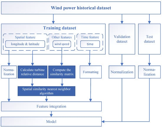
Figure 4.
Framework of proposed method.
It is worth mentioning that this paper differs from other prediction methods in that wind speed is indirectly input to the wind power prediction model as a feature for the following reasons:
- Considering wind speed as one of the important factors affecting the results of wind power prediction, small changes in wind speed may lead to significant changes in wind power []. The wind power prediction model still needs to take into account the impact caused by wind speed on the prediction.
- To eliminate the bias in wind power prediction due to wind speed prediction errors.
- To reduce the parameters for model training and improve the prediction efficiency.
3.2. Wavelet Transform-Based Frequency Domain Feature Extraction
The wavelet transform plays a crucial role in wind power prediction []. Compared with the traditional Fourier transform, it offers superior time resolution and allows for a more flexible selection of mother wavelet types, thereby enhancing signal analysis effectiveness and prediction accuracy. While the traditional Fourier transform may sacrifice time information when processing signals in the frequency domain, the wavelet transform retains both frequency and time information, making it more adept at analyzing intermittent and highly variable waveforms. There are two main types of wavelet transforms: discrete wavelet transform (DWT) and continuous wavelet transform (CWT) []. CWT can comprehensively capture all information within a given time-series signal, but it is computationally complex and challenging to implement []. In contrast, DWT utilizes discrete sampling and is more suitable for practical time series signal processing. Moreover, DWT effectively reduces computational complexity and mitigates the issue of information redundancy that may arise with CWT. Therefore, this paper opts for DWT, which is defined by the following Equation (7):
where is the scale parameter and n is the position parameter, is the wavelet basis function, and T is the length of the signal . Common wavelet basis functions are Haar wavelet, Daubechies wavelet, Symlet wavelet, and Coiflet wavelet. Among them, Haar wavelet is a function in the form of a square wave with the following mathematical formula:
where denotes the Haar wavelet basis function, which is defined in the interval . When t is in the interval , the wavelet function takes the value of 1, which indicates a positive spike; when t falls in the interval , the wavelet function takes the value of , which indicates a negative spike; in other intervals, the wavelet function takes the value of 0, which means no spike. In this paper, this wavelet basis function is chosen as the basis function of the wavelet transform, and the specific reasons will be explained in Section 4.5 (Experiments).
3.3. Relevant Models
3.3.1. Causal Convolutional Neural Network
Convolutional neural networks (CNNs) were initially developed for image recognition tasks. However, when it comes to time series data, researchers often lean towards recurrent neural networks (RNNs) or LSTM networks. Despite their effectiveness in various applications, RNNs and LSTMs encounter challenges such as high training memory requirements and prolonged training times. These issues become particularly pronounced when handling extensive sequential data, which is often the case in wind power prediction tasks. Therefore, causal convolution is introduced for wind power prediction task [].
Causal convolution is a specialized variant of the convolution operation designed for handling sequential data. It distinguishes itself by utilizing only current and preceding values from the input sequence to compute the output, excluding any information from future time steps. This is shown in Equation (9):
where N denotes the number of samples. Causal convolution predicts using , , ⋯, , which allows the network to learn the dependencies before and after the target moment. Figure 5 illustrates the structure of causal convolution.
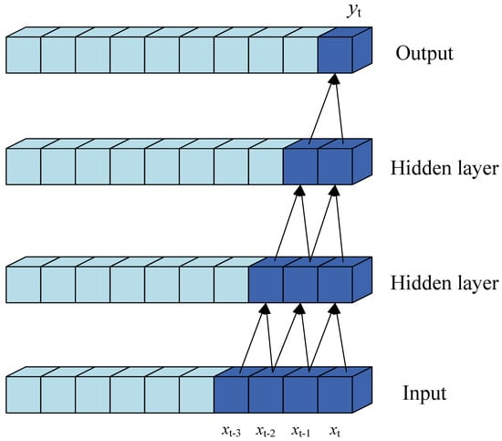
Figure 5.
The structure of causal convolution.
3.3.2. Deep-Learning-Based GRU
The gated recurrent unit (GRU) stands as a variant of RNN, similar to LSTM, renowned for its capacity to capture long-term dependencies []. Despite its simpler structure and fewer training parameters compared to LSTM, GRU exhibits comparable performance across various tasks. Illustrated in Figure 6, the GRU architecture comprises an update gate and a reset gate, governing the flow of information and memory retention. GRU, similar to LSTM, adeptly learns and retains both short-term and long-term correlations, enhancing its sequential data processing capabilities. The update gate modulates the incorporation of new input data with past memories, while the reset gate regulates the retention of historical information, facilitating the dynamic adjustment of information retention and forgetting. This gating mechanism endows GRU with greater flexibility in learning diverse sequential data patterns while achieving comparable performance with fewer parameters than LSTM. In the context of wind power prediction, characterized by intricate time dependencies among multiple variables, GRU enables the adaptive adjustment of historical information utilization and responsiveness to current inputs, thus enhancing the model’s capability in processing such sequential data.
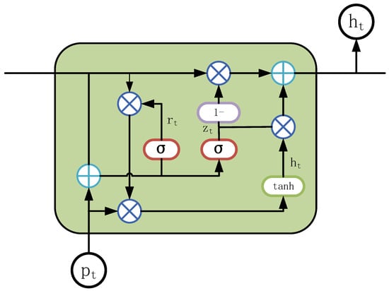
Figure 6.
The structure of GRU.
3.4. Wind Power Prediction Model with Multi-Feature Domain Learning
In this study, the Seq2Seq method serves as the foundational architecture of the model. The encoder component comprises two pathways: one harnesses a GRU network to glean spatio-temporal features, while the other extracts frequency-domain features via DWT. Subsequently, features acquired from both pathways are weighted, fused, and output as depicted below:
where denotes the encoder output, denotes the output of spatio-temporal data after GRU, and denotes the frequency domain features after DWT processing. In Section 4.6, we design experiments on weight values in detail.
In the decoder section, we introduce a feedforward module composed of two causal convolutional layers. This feedforward module embraces a causal convolutional structure and integrates a ReLU activation function, tailored to capture the nonlinear relationships among various factors, such as wind speed and wind power, thereby enhancing the model’s prediction accuracy. Towards the end of the feedforward module, we implement residual connections to preserve input information, which is then fused with processed data to facilitate the retention of historical information by the model. With this architecture, our model adeptly synthesizes spatio-temporal and frequency domain features, incorporating the nonlinear relationships of wind speed and wind power for more precise wind power predictions. The architecture of the model is illustrated in Figure 7.
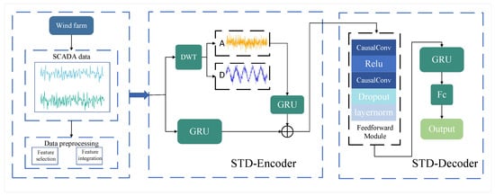
Figure 7.
The architecture of the model.
After preprocessing the one-dimensional SCADA data, it is fed into the STD-Encoder for both frequency domain and time domain feature extraction. In the frequency domain, discrete wavelet transform (DWT) is used to extract high-frequency signals, which are then processed by a gated recurrent unit (GRU). The resulting features are weighted and combined with those from the time domain. The decoder processes the information from the encoder and ultimately completes the prediction task.
Additionally, MFDnet utilizes the GRU-based Seq2Seq framework, which offers several advantages over other prediction methods:
- The Seq2Seq framework improves the input flexibility of the model and increases the generalizability of the model.
- GRU demonstrates superior capability in managing long-term dependencies while balancing the problem of vanishing gradients.
- The utilization of fewer model parameters results in decreased computational demands and hardware requirements.
4. Experiments
4.1. Evaluation Indicators
In this paper, the coefficient of determination (), mean absolute error (MAE), and root mean square error (RMSE) are employed as evaluation metrics for wind power forecasts. is a statistical measure used to assess the goodness of fit of a regression model. MAE assesses the average prediction error, while RMSE accentuates larger errors by squaring these deviations. The calculation of these metrics is outlined below:
where n is the number of sampling points, is the predicted value, and is the true power.
4.2. Relevant Work
The experiments in this paper are conducted utilizing the following hardware and software setup: NVIDIA GeForce RTX 3060 Laptop GPU, AMD Ryzen 7 5800H with a clock speed of 3.2 GHz, and PyCharm 2021 as the software environment. The paper proposes a short-term wind power prediction model based on multi-feature domain learning. Parameters for the model include a dropout size of 0.1 for the causal convolution, a convolution kernel size of 3, and the selection of Haar as the mother wavelet type for DWT. The experiment settings include 300 iterations, a learning rate of 0.001, optimization using the Adam optimizer, and setting the nearest neighbor k to 5, which specifies the number of turbines in each turbine ensemble to be 5.
Unlike other wind power prediction tasks that are based on a single wind farm, the dataset used in our experiments contains 200 different turbines. Considering that evaluating the combined prediction error of these 200 turbines as the overall prediction deviation for the wind farm might lead to compensating errors, we average the prediction errors of the 200 turbines to assess the accuracy of the wind farm’s power prediction.
4.3. Comparison with Traditional Methods
In this paper, we highlight the superiority of our proposed model by comparing it with a diverse range of classical models and state-of-the-art deep learning-based approaches. These comparisons encompass fundamental deep learning models such as multilayer perceptron (MLP) [], RNN [], GRU [], LSTM [], and LSTM-LSTM [], alongside deep learning models specifically tailored for wind power prediction, such as DST [] and STAN []. In addition to this, we have chosen the standard benchmark persistence model (denoted as PM in the Table 2) as the benchmark for the full text comparison. We used the coefficient of determination (), mean absolute error (MAE) and root mean square error (RMSE) as evaluation metrics. To enhance evaluation accuracy, all models underwent three rounds of testing within the same environment, and the results were averaged. The outcomes of these experiments are presented in Table 2, where the highest and lowest MAE or RMSE for each hour are highlighted for clarity.

Table 2.
Comparison of experimental results.
The experimental results indicate that the RMSE of the RNN is lower than that of our proposed model at the 1 h forecasting horizon. Moreover, our proposed method demonstrates smaller MAE and RMSE at most time intervals, substantiating the superior predictive capability of our model for wind power forecasting. In order to show the evaluated values of the different forecasting models more clearly at different time scales, bar charts have been employed for visualization, as shown in Figure 8, Figure 9 and Figure 10.
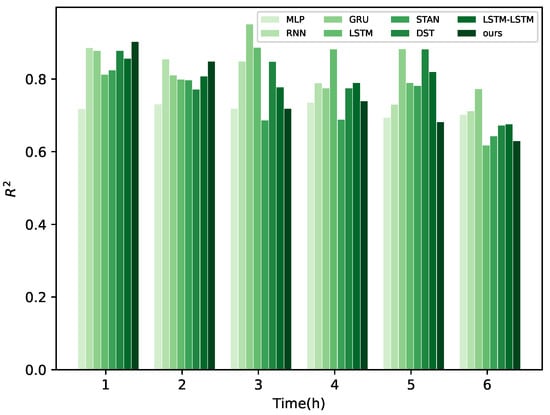
Figure 8.
for different methods.
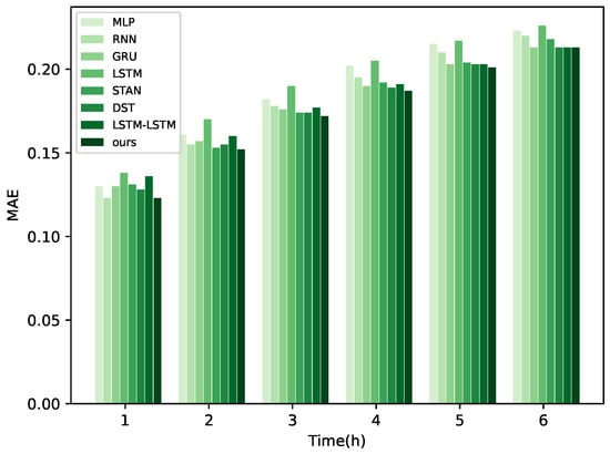
Figure 9.
MAE for different methods.
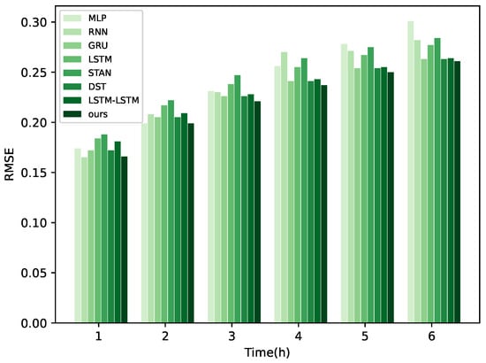
Figure 10.
RMSE for different methods.
In Figure 8, Figure 9 and Figure 10, a visual comparison of each model’s performance at different time points is presented. It is evident that the curve representing our model exhibits significant enhancement over other methods from 1 to 3 h. However, as time progresses, the superiority of our proposed model diminishes compared to other models. This phenomenon can be attributed to the model’s selection of the high-frequency component of the original signal during processing of frequency-domain information with GRU in the encoder. Typically, this component contains rapid variations or detailed information, corresponding to sudden changes in wind power characteristics. Moreover, high-frequency information also includes noise and other interference, posing challenges for the model in long-term feature extraction of wind power. Nevertheless, it is noteworthy that our model still demonstrates improvements compared to other methods, indicating its superior noise resistance and generalization capability. In Figure 11, the forecast performance of a wind farm comprising 200 turbines is shown, indicating that the actual results are closely aligned with the model’s predictions.
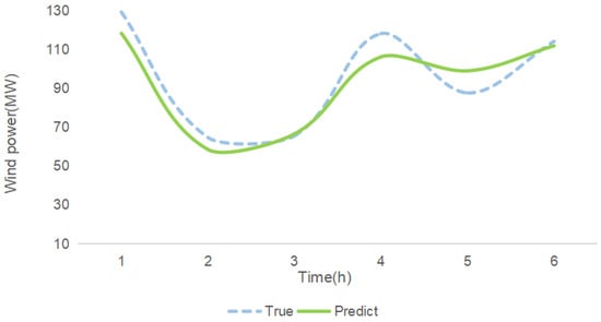
Figure 11.
Comparison of actual data and best model predictions.
In summary, we attribute the superior performance of our method in short-term wind power prediction tasks to the following possible factors:
- The Seq2Seq framework captures deeper temporal dependencies than simple prediction methods such as LSTM or GRU.
- The introduction of DWT to extract frequency domain information improves the utilization of information by fusing the idea of spatio-temporal and frequency domain features.
- The use of the embedding method, which introduces individual turbine identities as features, enables the model to learn the differences between turbines and predict based on these differences, leading to a more accurate prediction of future power generation.
4.4. K Tuning Experiment
This section delves into examining the impact of the value of k on the accuracy of the prediction task within the SSNN. Figure 12 shows the autocorrelation of wind speeds for 20 turbines at lag times of 1 to 4 h, revealing strong correlations over short periods. This means that the wind resources owned by these turbines are similar and the number of turbine groups should be controlled to a small value. And since the autocorrelation coefficients of the turbines are all close to each other, this indicates that the number of turbines constituting the turbine group should be approximately the same. Therefore, the number of turbine groups in this paper is controlled to be the same constant k. To effectively verify the influence of the value of k on the accuracy of the final prediction task, this paper has conducted the following test, setting the range of k to be a positive integer interval from 1 to 10, with all other conditions of the test remaining the same. The final result is the average result after three trials as shown in Table 3, Table 4 and Table 5.
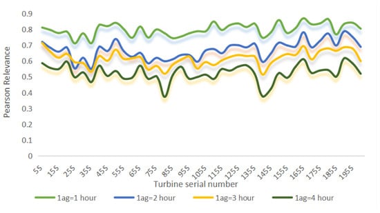
Figure 12.
Correlation of wind speeds for different turbines at different lag times.

Table 3.
of different values of k.

Table 4.
MAE of different values of k.

Table 5.
RMSE of different values of k.
is closest to 1, and both MAE and RMSE predictions are minimized when , indicating optimal performance. Moreover, there is a discernible decrease in prediction accuracy as k deviates from this optimal value . This outcome can be attributed to the methodology employed in this paper, where turbine groups derived from the k-nearest neighbors serve as feature inputs for model training. During this training process, the turbine group data act as mutual constraints, ensuring that the wind power of a turbine group remains similar. When k is small, these turbines fail to exert significant constraints, resulting in poorer predictions. Conversely, when k exceeds the optimal value, a larger number of unrelated turbines are included, leading to misjudgments by the model and subsequent declines in prediction accuracy.
4.5. Effects of Mother-Wavelet Selection
This paper presents an algorithm utilizing the Haar wavelet basis functions within the wavelet transform to extract high- and low-frequency components. Actually, the DWT includes various wavelet basis functions, such as the Daubechies (db) wavelet, Symlet (sym) wavelet, and Coiflet (coif) wavelet. The selection of different mother wavelets can influence the processing of time series data to some extent []. To delve deeper into the implications of mother wavelet selection, we conducted a case study involving different types of wavelet basis functions. These functions can be represented in a general form:
where are the filter coefficients and is the wavelet basis function; the optional N determines its specific properties and support length.
In this paper, we selected commonly used wavelet basis functions, namely sym2, Haar, db2, and coif1. It is noteworthy that each of these wavelets possesses distinct advantages. For instance, the Daubechies wavelet boasts tight support and orthogonal properties, rendering it proficient in accurately capturing both short-term and long-term features within the signal. Symlet is characterized by greater symmetry compared to other wavelets, exhibiting minimal asymmetry and the highest number of vanishing moments for a given compact support, thus effectively handling asymmetric signals []. Coiflet wavelets are particularly well-suited for analyzing transient, time-varying signals, making them ideal for processing non-smooth signals and signals with pronounced singularities [].
To assess the impact of various mother wavelets on the prediction outcomes, three alternative wavelet basis functions were employed in lieu of the Haar wavelet for experimentation. Subsequently, the prediction performance metrics of , MAE and RMSE are evaluated and compared. The results are illustrated in Figure 13, Figure 14, Figure 15, Figure 16, Figure 17, Figure 18, Figure 19, Figure 20, Figure 21, Figure 22, Figure 23 and Figure 24.
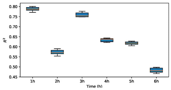
Figure 13.
for sym2.
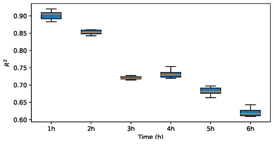
Figure 14.
for Haar.
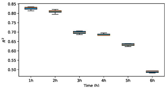
Figure 15.
for db2.
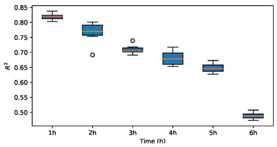
Figure 16.
for coif1.
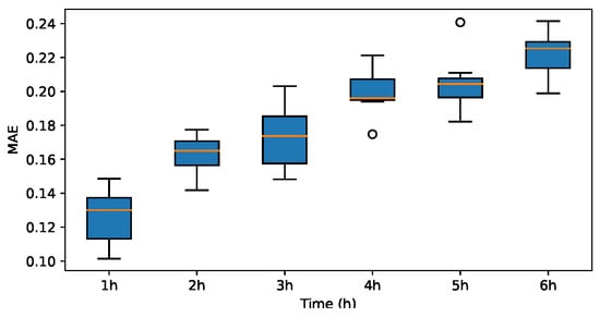
Figure 17.
MAE for sym2.
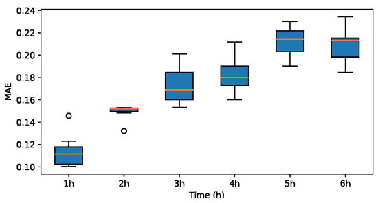
Figure 18.
MAE for Haar.
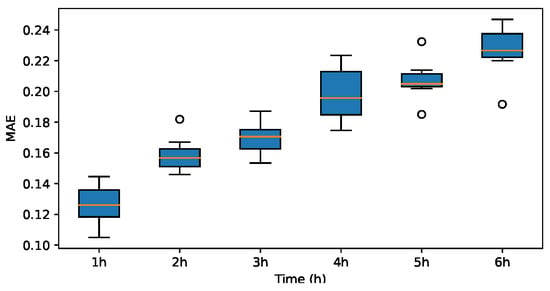
Figure 19.
MAE for db2.
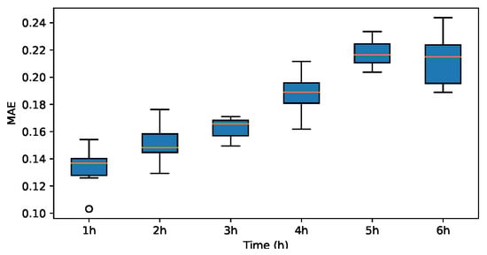
Figure 20.
MAE for coif1.
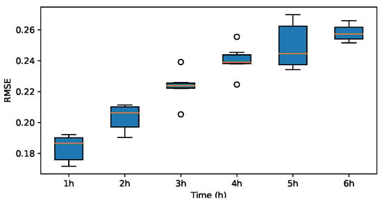
Figure 21.
RMSE for sym2.
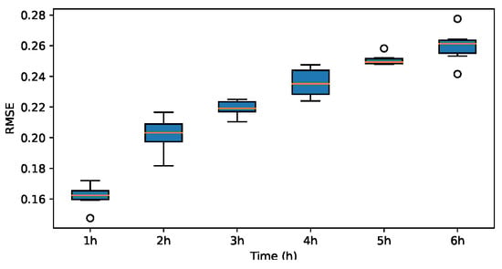
Figure 22.
RMSE for Haar.
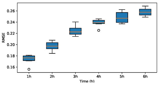
Figure 23.
RMSE for db2.
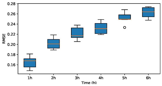
Figure 24.
RMSE for coif1.
The results indicate that the MAE and RMSE values obtained using the Haar-based DWT are consistently lower compared to those achieved with all other mother wavelets, and the value is higher than those of the other mother wavelets. Therefore, it can be concluded that the widely adopted Haar wavelet basis function is more suitable for wind power prediction tasks in this context.
4.6. Weighted Design Experiment
In Section 3.2, a weighted summation method is proposed to integrate information from both the frequency and spatio-temporal domains. This weighted approach is designed to regulate the influence of each domain on the final prediction results. As the parameter increases, high-frequency features in the frequency domain may exert a greater influence on the results. However, this also amplifies the interference from noise present in the high-frequency signals, thereby affecting the prediction more significantly. Conversely, as decreases, features processed by the encoder tend to align more closely with the long-term trend.
To enhance the rigor of the weighting design, this section conducts experiments with various weighting parameter configurations, with , MAE and RMSE selected as the evaluation metric. Figure 25, Figure 26 and Figure 27 present the results of these experiments. Nine different weight combinations are compared in this paper, all summing to 1. It is observed that at the 1-hour mark, the combination of = 0.9 and = 0.1 demonstrates superior prediction performance compared to other models. Over time, the impact of different weights on the prediction results diminishes. Beyond the 3-hour mark, the disparities among the prediction results under different weight configurations become negligible, as shown in Figure 26 and Figure 27.
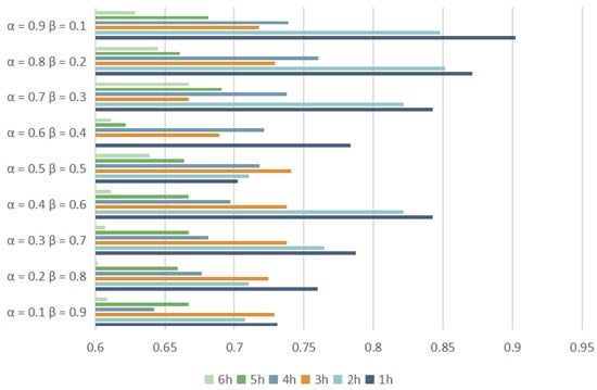
Figure 25.
with different weights.
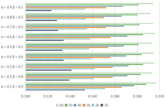
Figure 26.
MAE with different weights.
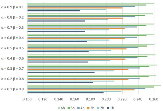
Figure 27.
RMSE with different weights.
Consequently, this paper selects the weights = 0.9 and = 0.1. These parameters are deemed optimal for the weighted summation method.
4.7. Ablation Experiment
Based on the aforementioned experimental outcomes, our proposed model demonstrates superior performance on the public dataset. To delve into the validity of SSNN, DWT frequency domain processing, and the feedforward module within our proposed model, we conducted an ablation experiment outlined in Table 6. It is worth mentioning that we chose the Seq2Seq framework with both encoder and decoder as GRU as the baseline.

Table 6.
Ablation protocol.
The experimental results are presented in Table 7, Table 8 and Table 9. Ablation experiments CM1, CM2, and CM3 demonstrate that our MFDnet outperforms when using individual modules alone. Conversely, experiments CM4, CM5, and CM6 reveal that SSNN performs the best in our model, followed by the feedforward module, and lastly, DWT. Further analysis combined with CM2 results suggests a mismatch issue between DWT and the feedforward module. This mismatch arises from the feedforward module learning noise characteristics. Integrating SSNN into the model helps alleviate this misalignment by enhancing similarity features between turbines, thereby mitigating the noise effects introduced by DWT on the final prediction results to some extent. This is corroborated by the relatively poor performance of CM1 alone.

Table 7.
for ablation experiments.

Table 8.
MAE for ablation experiments.

Table 9.
RMSE for ablation experiments.
Comparing the MAE and RMSE results of the baseline and MFDnet, this study concludes the following: MFDnet exhibits significant improvements in wind power prediction compared to the GRU-based Seq2Seq framework. Specifically, MFDnet improves by 10.4%, reduces MAE by 4.1% and RMSE by 3.6% at the 1-hour mark, and improves by 5.5%, reduces MAE by 1.6% and RMSE by 1.7% on average across the 6-h prediction task.
5. Conclusions
In this research, we developed a short-term wind power forecasting model that intergrates multiple feature domains aimed at enhancing the accuracy of short-term wind power predictions. The crux of the model involves utilizing data from wind turbines within a wind farm to predict the wind farm’s power output. At the input stage, the model captures inter-turbine correlation features along with spatial and temporal features through a spatial similarity-based nearest neighbor algorithm, which forms the input to the model. By introducing a strategy of multi-feature domain fusion, the spatial, temporal, and frequency domain features are designed to complement each other. On the feature extraction end, a feedforward module captures nonlinear relationships, enabling the model to improve its adaptability in wind power forecasting by analyzing both long-term and short-term dependencies in sequential data. Comprehensive testing on an open wind power dataset has shown that the MFDnet model possesses significant efficacy, outperforming other advanced models such as STAN and DST in two distinct evaluation metrics for short-term wind power forecasting tasks. Additionally, compared to the persistence model, MFDnet achieved an average reduction of 33.7% in MAE and 22.3% in RMSE, while improves by 4.8%.
Future work can be summarized in two main directions. Firstly, under the condition of obtaining more data, to expand the prediction from a single wind farm to different wind farms’ power forecasts, thereby increasing the model’s generalizability. Secondly, to further consider the trend and fluctuation details of wind power predictions, refining the proposed forecasting method to improve accuracy and achieve ultra-short-term wind power prediction.
Author Contributions
Methodology, X.H.; software, X.H. and Y.X.; validation, Y.X. and J.Y.; formal analysis, J.Y. and Y.X.; data curation, Y.X.; writing—original draft, Y.X., X.H. and J.Y.; writing—review and editing, J.Y., Y.X. and X.H.; funding acquisition, J.Y. All authors have read and agreed to the published version of the manuscript.
Funding
This work was supported in part by Tianjin University of Technology under Project YBXM2310.
Institutional Review Board Statement
Not applicable.
Informed Consent Statement
Not applicable.
Data Availability Statement
The original contributions presented in the study are included in the article, further inquiries can be directed to the corresponding author.
Conflicts of Interest
The authors declare no conflicts of interest.
References
- Li, H.; Liu, L.; He, Q. A Spatiotemporal Coupling Calculation Based Short-Term Wind Farm Cluster Power Prediction Method. IEEE Access 2023, 11, 131418–131434. [Google Scholar] [CrossRef]
- Sun, Y.; Yang, J.; Zhang, X.; Hou, K.; Hu, J.; Yao, G. An Ultra-short-term wind power forecasting model based on EMD-EncoderForest-TCN. IEEE Access 2024. Available online: https://ieeexplore.ieee.org/document/10460523 (accessed on 5 March 2024). [CrossRef]
- Li, M.; Yang, M.; Yu, Y.; Li, P.; Wu, Q. Short-Term Wind Power Forecast Based on Continuous Conditional Random Field. IEEE Trans. Power Syst. 2024, 39, 2185–2197. [Google Scholar] [CrossRef]
- Zhu, J.; Su, L.; Li, Y. Wind power forecasting based on new hybrid model with TCN residual modification. Energy AI 2022, 10, 100199. [Google Scholar] [CrossRef]
- Yang, M.; Wang, D.; Xu, C.; Dai, B.; Ma, M.; Su, X. Power transfer characteristics in fluctuation partition algorithm for wind speed and its application to wind power forecasting. Renew. Energy 2023, 211, 582–594. [Google Scholar] [CrossRef]
- Wang, D.; Yang, M.; Zhang, W. Wind Power Group Prediction Model Based on Multi-Task Learning. Electronics 2023, 12, 3683. [Google Scholar] [CrossRef]
- Stathopoulos, C.; Kaperoni, A.; Galanis, G.; Kallos, G. Wind power prediction based on numerical and statistical models. J. Wind. Eng. Ind. Aerodyn. 2013, 112, 25–38. [Google Scholar] [CrossRef]
- Milligan, M.; Schwartz, M.; Wan, Y. Statistical Wind Power Forecasting Models: Results for U.S. Wind Farms; Preprint. 2003. Available online: https://api.semanticscholar.org/CorpusID:11737140 (accessed on 1 May 2003).
- Peng, X.; Chen, Y.; Cheng, K.; Zhao, Y.; Wang, B.; Che, J.; Wen, J.; Lu, C.; Lee, W. Wind Power Prediction for Wind Farm Clusters Based on the Multi-feature Similarity Matching Method. In Proceedings of the 2019 IEEE Industry Applications Society Annual Meeting, Baltimore, MD, USA, 29 September–3 October 2019; pp. 1–11. [Google Scholar]
- Deepak, P.L.; Ramkumar, G.; Sajiv, G. Improved Wind Power Generation Prediction through Novel Linear Regression over Ridge Regression. In Proceedings of the 2024 2nd International Conference on Advancement in Computation & Computer Technologies (InCACCT), Gharuan, India, 2–3 May 2024; pp. 46–50. [Google Scholar]
- Zeng, J.; Qiao, W. Support vector machine-based short-term wind power forecasting. In Proceedings of the 2011 IEEE/PES Power Systems Conference and Exposition, Phoenix, AZ, USA, 20–23 March 2011; pp. 1–8. [Google Scholar]
- An, G.; Jiang, Z.; Cao, X.; Liang, Y.; Zhao, Y.; Li, Z.; Dong, W.; Sun, H. Short-Term Wind Power Prediction Based On Particle Swarm Optimization-Extreme Learning Machine Model Combined With Adaboost Algorithm. IEEE Access 2021, 9, 94040–94052. [Google Scholar] [CrossRef]
- Zhou, B.; Ma, X.; Luo, Y.; Yang, D. Wind Power Prediction Based on LSTM Networks and Nonparametric Kernel Density Estimation. IEEE Access 2019, 7, 165279–165292. [Google Scholar] [CrossRef]
- Hao, J.; Zhu, C.; Guo, X. Wind Power Short-Term Forecasting Model Based on the Hierarchical Output Power and Poisson Re-Sampling Random Forest Algorithm. IEEE Access 2020, 9, 6478–6487. [Google Scholar] [CrossRef]
- Deng, W.; Dai, Z.; Liu, X.; Chen, R.; Wang, H.; Zhou, B.; Tian, W.; Lu, S.; Zhang, X. Short-Term Wind Power Prediction Based on Wind Speed Interval Division and TimeGAN for Gale Weather. In Proceedings of the 2023 International Conference on Power Energy Systems and Applications (ICoPESA), Nanjing, China, 24–26 February 2023; pp. 352–357. [Google Scholar]
- Hossain, M.A.; Gray, E.; Lu, J.; Islam, M.R.; Alam, M.S.; Chakrabortty, R.; Pota, H.R. Optimized Forecasting Model to Improve the Accuracy of Very Short-Term Wind Power Prediction. IEEE Trans. Ind. Inform. 2023, 19, 10145–10159. [Google Scholar] [CrossRef]
- Fan, W.; Miao, L.; An, Y.; Chen, D.; Zhong, K. Wind Farm Ultra Short Term Power Prediction Considering Attention Mechanism and Historical Data of Wind Farm Internal Units. In Proceedings of the 2024 6th Asia Energy and Electrical Engineering Symposium (AEEES), Chengdu, China, 28–31 March 2024; pp. 1121–1125. [Google Scholar]
- Hu, J.; Meng, W.; Tang, J.; Zhuo, Y.; Rao, Z.; Sun, S. Short-Term Wind Power Prediction under Cold Wave Weather Conditions based on Neural Prophet. In Proceedings of the 2024 7th International Conference on Advanced Algorithms and Control Engineering (ICAACE), Shanghai, China, 1–3 March 2024; pp. 1262–1266. [Google Scholar]
- Zhu, N.; Wang, Y.; Yuan, K.; Yan, J.; Li, Y.; Zhang, K. GGNet: A novel graph structure for power forecasting in renewable power plants considering temporal lead-lag correlations. Appl. Energy 2024, 364, 123194. [Google Scholar] [CrossRef]
- Ding, Y. Data Science for Wind Energy; Chapman & Hall/CRC Press: Boca Raton, FL, USA, 2019; Available online: https://api.semanticscholar.org/CorpusID:199102989 (accessed on 24 May 2019).
- Yu, C.; Yan, G.; Yu, C.; Zhang, Y.; Mi, X. A multi-factor driven spatiotemporal wind power prediction model based on ensemble deep graph attention reinforcement learning networks. Energy 2023, 263, 126034. [Google Scholar]
- Kim, Y.; Kim, M.K.; Fu, N.; Liu, J.; Wang, J.; Srebric, J. Investigating the Impact of Data Normalization Methods on Predicting Electricity Consumption in a Building Using different Artificial Neural Network Models. Sustain. Cities Soc. 2024, 105570. [Google Scholar] [CrossRef]
- Li, J.; Armandpour, M. Deep Spatio-Temporal Wind Power Forecasting. In Proceedings of the ICASSP 2022-2022 IEEE International Conference on Acoustics, Speech and Signal Processing (ICASSP), Singapore, 23–27 May 2022; pp. 4138–4142. [Google Scholar]
- Hochreiter, S.; Schmidhuber, J. Long Short-Term Memory. Neural Comput. 1997, 9, 1735–1780. [Google Scholar] [CrossRef] [PubMed]
- Xiong, Z.; Wang, C.; Zhao, Y.; Deng, D.; Liu, H. A Grouping Method of Sea Battlefield Targets Based on The Improved Nearest Neighbor Algorithm. In Proceedings of the 2022 IEEE International Conference on Unmanned Systems (ICUS), Guangzhou, China, 28–30 October 2022; pp. 298–302. [Google Scholar]
- Erdem, E.; Shi, J. ARMA based approaches for forecasting the tuple of wind speed and direction. Appl. Energy 2011, 88, 1405–1414. [Google Scholar] [CrossRef]
- Percival, D.B.; Walden, A.T. Wavelet Methods for Time Series Analysis. In Cambridge Series in Statistical and Probabilistic Mathematics, 4th ed.; Cambridge University Press: Cambridge, UK, 2000. [Google Scholar]
- Ahn, E.; Hur, J. A short-term forecasting of wind power outputs using the enhanced wavelet transform and arimax techniques. Renew. Energy 2023, 212, 394–402. [Google Scholar] [CrossRef]
- Zhang, W.; Lin, Z.; Liu, X. Short-term offshore wind power forecasting—A hybrid model based on Discrete Wavelet Transform (DWT), Seasonal Autoregressive Integrated Moving Average (SARIMA), and deep-learning-based Long Short-Term Memory (LSTM). Renew. Energy 2022, 185, 611–628. [Google Scholar] [CrossRef]
- Yang, Y.; Zhang, H.; Peng, S.; Su, S.; Li, B. Wind Power Probability Density Prediction Based on Quantile Regression Model of Dilated Causal Convolutional Neural Network. Chin. J. Electr. Eng. 2023, 9, 120–128. [Google Scholar] [CrossRef]
- Chung, J.; Gulcehre, C.; Cho, K.; Bengio, Y. Empirical Evaluation of Gated Recurrent Neural Networks on Sequence Modeling. arXiv 2014, arXiv:1412.3555. [Google Scholar]
- Velasco, L.C.P.; Serquiña, R.P.; Zamad, M.S.A.A.; Juanico, B.F.; Lomocso, J.C. Week-ahead Rainfall Forecasting Using Multilayer Perceptron Neural Network. Procedia Comput. Sci. 2019, 161, 386–397. [Google Scholar] [CrossRef]
- Liu, M.; Ding, L.; Bai, Y. Application of hybrid model based on empirical mode decomposition, novel recurrent neural networks and the ARIMA to wind speed prediction. Energy Convers. Manag. 2021, 233, 113917. [Google Scholar] [CrossRef]
- Liu, X.; Lin, Z.; Feng, Z. Short-term offshore wind speed forecast by seasonal ARIMA—A comparison against GRU and LSTM. Energy 2021, 227, 120492. [Google Scholar] [CrossRef]
- Hu, Z.; Gao, Y.; Ji, S.; Mae, M.; Imaizumi, T. Improved multistep ahead photovoltaic power prediction model based on LSTM and self-attention with weather forecast data. Appl. Energy 2024, 359, 122709. [Google Scholar] [CrossRef]
- Fu, X.; Gao, F.; Wu, J.; Wei, X.; Duan, F. Spatiotemporal Attention Networks for Wind Power Forecasting. In Proceedings of the 2019 International Conference on Data Mining Workshops (ICDMW), Beijing, China, 8–11 November 2019; pp. 149–154. [Google Scholar]
- Moradi, M. Wavelet transform approach for denoising and decomposition of satellite-derived ocean color time-series: Selection of optimal mother wavelet. Adv. Space Res. 2022, 69, 2724–2744. [Google Scholar] [CrossRef]
- Shen, Y.; Sun, J.; Yang, X.; Liu, P. Symlets Wavelet Transform based Power Management of Hybrid Energy Storage System. In Proceedings of the 2020 IEEE 4th Conference on Energy Internet and Energy System Integration (EI2), Wuhan, China, 30 October–1 November 2020; pp. 2556–2561. [Google Scholar]
- Patwary, R.; Datta, S.; Ghosh, S. Harmonics and interharmonics estimation of a passive magnetic fault current limiter using Coiflet Wavelet transform. In Proceedings of the 2011 International Conference on Communication and Industrial Application, Kolkata, India, 26–28 December 2011; pp. 1–6. [Google Scholar]
Disclaimer/Publisher’s Note: The statements, opinions and data contained in all publications are solely those of the individual author(s) and contributor(s) and not of MDPI and/or the editor(s). MDPI and/or the editor(s) disclaim responsibility for any injury to people or property resulting from any ideas, methods, instructions or products referred to in the content. |
© 2024 by the authors. Licensee MDPI, Basel, Switzerland. This article is an open access article distributed under the terms and conditions of the Creative Commons Attribution (CC BY) license (https://creativecommons.org/licenses/by/4.0/).