1. Introduction
Overdependence on the conventional means of energy generation will take society nowhere except for the death of energy and climatic hazards, which not only influence the environment but also impact the different types of ecosystems, and a glimpse of the same is already being seen in terms of forest land shrinkage, migration of biotic components from their original habitat, reduction in the soil fertility, forest infernos, urbanization, decreasing number of hotspots, wildlife–human conflicts, and the contamination of water sources. The quest should be for alternative measures rather than investing a vast amount of capital into longer energy payback schemes, such as carbon capture storage, whose success chance is 1 out of 9. In the subsequent paragraphs, three major aspects were considered to critically examine the torrefaction process based on relative merit.
The task is to bring the unexplored division of biomass into the main energy stream; it has been recently involved in power generation, but it is not as effective as its counterparts (solid biomass). The loose biomass that is characterized by its lower bulk density, higher moisture content, high oxygen-to-carbon ratio, lower grinding ability, a large amount of tar, and a higher transportation cost can be valorized if the technique of optimization is combined with preprocessing techniques. One of the methodologies to counter this problem is blending biomass with higher exergy ratio fuels to optimize the prevailing system or vary the main parameters to make the thermochemical process effective and efficient [
1]. The blending, or co-fired, technique is a relatively clean technology that reduces the overall fuel consumption cost, tar content, and emission of greenhouse gases, albeit it also relies on fuel quality. The marginal effect on the effectiveness of the thermochemical process can be materialized by either drying or reducing the size of the biomass. To upgrade the quality of feedstock, torrefaction also presents another facet in the context of fuel effectiveness and material handling [
2]. Torrefaction, or pre-treatment, is a thermal process that involves the prior thermal heating (200–250 °C) of biological material in a reactor under an inert atmosphere to improve its physio-chemical properties. Regarding the same, the impact of time and temperature on the effectiveness of the torrefaction process was examined using Austrian pine waste. It was reported that temperature had a more dominating impact on determining energy and mass yields than time. It was concluded that the grain orientation as well as longitudinal cracks were altered after the torrefaction of the Austrian pine. In addition, the chemical reaction pathway of the torrefied sample also deviated from its raw form. It was seen that the nucleation growth and high-order diffusion reaction led to drastic changes in the activation energies of the Austrian pine waste [
3]. However, the physical characteristic of different feedstocks in a co-fired technology also impacts the efficacy of the pre-treatment process. It was reported that the addition of sulphuric acid along with an increasing ramping rate synergized the process of wet torrefaction of sugarcane bagasse. It was noticed that the calorific content of the substrate was increased by 20.3% through hydrothermal carbonization. Albeit, the thermodynamics of the process were omitted during the carbonization of the biomass [
4]. The energetic aspect was covered while performing the torrefaction of beechwood [
5]. It was observed that the increasing residence time and mass loss of beechwood in a reactor enhanced the exothermic heat of the reaction to 199 J∙g
−1. A sample of 10% moisture underwent torrefaction for 40 min at 280 °C, which resulted in a reduction of heat consumption by 28.49%. It was also reported that residence time played a more significant role than temperature in estimating heat consumption during the torrefaction process [
5]. The research was rather based on the quantitative aspect of torrefaction than discussing the rationale behind energy fluctuation during the pre-treatment process. In another study, it was reported that the increasing torrefaction temperature would cause a simultaneous reduction in hydroxyl and carboxyl groups and an increase in C=C bonds. However, the activation energy of the thermal decomposition of Yunnan pine remained in the range of 69–129 kJ∙mol
−1 even after the torrefaction process [
6]. Although the extensive analysis was performed, the change in the reaction pathway during torrefaction was not revealed, which allowed the researchers to determine the deviation in the activation energy of the biomass from the change in the degree of torrefaction. In a similar type of study on the microalga
Chlorella vulgaris, torrefaction at 300 °C provided the maximum change in the calorific value if the substrate was kept inside a fixed bed tubular reactor for 30 min. It was observed that the torrefaction also changed the degradation rate of polymers present in the microalgae. The rate of degradation of remaining protein was impeded, while at the same time, the thermal degradation rate of lipids gained momentum [
7]. The samples of oil palm fiber and Eucalyptus underwent the pre-treatment process in an N
2 and air atmosphere at 250 °C, 275 °C, 300 °C, 325 °C, and 350 °C. Unlike Eucalyptus, based on energy and solid yield and an energy–mass co-benefit index (EMCI), the oil palm fiber would provide a relatively good solid yield only if it is pre-treated in an N
2 atmosphere at 300 °C for 1 h [
8]. In another study, it was reported that the heating value would be at its maximum at 300 °C if the sample of bagasse is heated for 90 min. Relatively to bagasse, sawdust, and water hyacinth, torrefied peanut husks rapidly elevated the bed temperature of a spout-fluid bed combustor. The reason provided by the researchers was its lower moisture content; however, the main factors that affect combustion characteristics were missing [
9]. Torrefaction of a Lauan block at 280 °C for 120 min enhanced the calorific value of the sample by more than 40%, but for the same operating condition, the solid yield was merely 50%. Considering grinding ability and energy yield as the decision-making factors, it was recommended to process the wooden block at 250 °C for 60 min [
10]. In the case of agricultural biomass waste, torrefaction of mesocarp fiber and kernel shell provided an energy yield of higher than 95% at 300 °C for 30 min; however, the solid yield, which is one of the key constraints while optimizing the torrefaction process, was omitted from the discussion [
11].
Material properties also play a relevant role during the thermal decomposition of biomass. As was reported beforehand, morphology and polymeric composition also get permuted with torrefaction; the residence time of fluid is dilated for the large-size particles of biomass to trigger the secondary reactions of the product of the primary reactions [
12]. The grindability of torrefied wood pellets and their raw form was determined using a ball mill. According to the DIN 66145 standard, the particle size distributions of both torrefied and raw wood pellets were estimated through the RRSB (Rosin, Rammler, Sperling, and Bennett) model and it was noticed that the raw wood pellets required relatively high specific power as compared to its torrefied pellets [
13]. The torrefaction of Norway spruce sawdust of less than 4 mm in size below 230 °C for 60 min led to a mass loss of 2.8%, which resulted in a more than 21% reduction in specific energy consumption [
14]. In another relevant study, it was quoted that the energy required for grinding dropped significantly as the torrefaction temperature increased [
15].
Apart from changing the operating condition or trying hit-and-trial methods to obtain the desirable results based on energy and mass yield, machine learning can also be employed to shift the paradigm from the conventional scheme to a unique approach to appraise the pre-treatment process differently. The artificial neural network (ANN) and Response Surface Methodology (RSM) were employed to optimize the torrefaction process conditions, such as temperature, time, and blending ratio. It was estimated that the blending ratio of coal-to-torrefied biomass at 300 °C for 45 min would be 50:50 [
16]. Norwegian forest residues (birch branches) underwent torrefaction within the narrow temperature range of 275–278 °C for 30 min. The derived results were compared and validated using the in-built Redlich–Kwong–Soave model (RKS) in Aspen Plus. It was concluded that the evaporation of water took around 76–80% of the total heat and it was not recommended to process the biomass at higher temperatures, owing to a reduction in energy efficiency with the increase in pre-processing temperature. The derived results were based on the atmospheric pressure and any perturbation in reactor pressure was absent. This work lacks the execution of torrefaction with a real parameter as the mass and energy yields, along with the composition of volatiles, also rely on the state properties (total pressure and local temperature) of the torrefaction reactor [
17], which was thoroughly covered by Dhaundiyal and Toth (2023) [
18]. In another study, beech, pine, wheat straw, and willow were thermally pre-processed at the temperature range of 200–300 °C for 10–300 min. The statistical method of least square regression, was used to perform the numerical simulation of torrefaction. The work was based on the chemical kinetic model and inspired by the two-step reaction model of Blasi and Lazentta [
19] that overlooks the autocatalytic reactions which can be influenced by the heating rate and residence time of fluid; in other words, kinetic constants count strongly on the experimental conditions. It was also concluded that temperature had a more dominant effect on the elemental composition of the biomass than the resident time, which is not always true [
20]. The Malaysian species (Acacia, Macaranga, and oil palm biomass (oil palm trunk and empty fruit bunch (EFB)) were thermally treated at 200 °C, 250 °C, and 300 °C for 15 min, 30 min, and 45 min, respectively. Response surface methodology was employed to optimize the torrefaction process so that the maximum energy yield could be obtained at the cost of minimum solid yield. The optimized operational solution of EFB was estimated to be 230 °C for 45 min, whereas the numerical solution obtained for the Acacia and Macaranga species were 260 °C and 280 °C for 30 min and 45 min, respectively [
21]. Through the application of artificial intelligence, a nonlinear predictive model was developed to estimate the gross heating value of 250 biomass samples, which were trifurcated into a training set (174 samples), validation set (38 samples), and testing set (38 samples). The application of the training set was to train the artificial neural network (ANN) and to control the over-fitting issues, whereas the validation dataset function was to check the generalization ability of the ANN model and to prevent the compilation of the force-fitting [
22]. In another similar sort of work, a hybrid algorithm between the particle swarm optimization (PSO) technique and the support vector machine (SVM) was employed to predict the higher heating value of biomass, but this metaheuristic technique does not validate that the globally optimal solution could exist for a particular class of problem; in other words, it strongly depends on a set of generated random variables. Albeit, it is a good technique when the information about the problem is limited [
23]. In another work, the optimization of hempseed oil yield was carried out by combining the ANN with a genetic algorithm (GA). Two mathematical models were proposed to correlate the hempseed oil yield with extraction temperature and time. A second-order polynomial equation was used to express oil yield as a function of explanatory variables [
24]. In a similar study, the higher heating value of around 12 different types of biomass residues was examined using the ANN model. It was claimed that the ANN model provides a reasonable performance by curtailing the fitting correlation for larger databases. Conversely, an empirical correlation model fits systematically with the fitted data for a similar size of database [
25].
Based on the past findings, it was seen that the previous work predominately emphasized the hit-and-trial techniques and particle-size distribution to determine the optimized solution, and the nuance of machine learning is pivoted around the conventional linear regression models. However, the methods covered in [
15,
16,
17,
18,
19,
20,
21,
22,
23,
24,
25] provided the different aspects of machine learning, but the basic tenet of formulating the problem is almost the same. In this article, the thermal pre-treatment of pine waste was examined through the simulated annealing method.
2. Materials and Methods
The methodology and method required during the analysis of the torrefaction process are divided into two sub-headings: Biomass processing and mathematical model. As a feedstock, the pine cones underwent thermal pre-processing before investigating their physio-chemical properties.
2.1. Biomass Processing
The pine waste was collected from Elisabeth Park, Godollo, Hungary. The coordinates of the area of collection of pine waste are 47.60 N and 19.33 E. The ultimate and proximate analyses were carried out at the Institute of Agricultural Engineering, National Agricultural and Innovation Centre, Godollo, Hungary. The net 9.11 kg of pine cone was collected and ground by a 1.49 kW rotor milling machine with a 6-disc rotor (Retsch SM 2000, Haan, Germany) to allow it to pass through a 1.5 mm sieve. The size of the hopper was 80 mm × 80 mm. The feeding rate of pine cones was in the range of 0.05–0.08 kg∙min
−1. The measured bulk density of the pine cones was 295.60 kg∙m
−3. The physical conversion efficiency of the pine cones was 53.34%. The average *energy consumption to mill the pine cones was 76.55 kW∙h/kg (
$7.58/kg). For torrefaction purposes, around 10 g of powder-form pine cone (
Pinus nigra) was thermally processed by improvising a programmable Joule heating system (Nabertherm Gmbh, Lilienthal, Germany). The drawing of the proposed torrefaction unit is shown in
Figure 1. The *energy required for the thermal pre-treatment process was 7 kW∙h/kg (
$ 0.53/kg). The energy consumption of the heating system and grinder was estimated using a multifunction analyzer (EMD, Contrel Electtronica, Lombardy, Italy).
*—Based on the electricity rate in Hungary. Note: The detailed description of elemental and calorimetric measurements is provided in
Appendix A.
The thermal pre-treatment was carried out at 210 °C, 220 °C, 230 °C, 240 °C, and 250 °C in the presence of nitrogen gas. The residence time for each quasistatic process was 5 min, 10 min, and 15 min. The gas meter (Ganz 2000, Budapest, Hungary) was used to monitor the flow rate of N2 gas. The volumetric flow rate considered for thermal pre-treatment was 0.7 L∙s−1, whereas the pressure head created by the inert gas was 15.29 m of the water column. The average dynamic pressure head inside the reactor was 1.04 m. The fugacity coefficient of inert gas inside the reactor was assumed to be unity, owing to low-pressure application.
The polymeric composition of the torrefied, as well as the raw pine cones, are provided in
Table 1. The sample size for polymeric composition was 2–3 g. The methodology used to determine the percentage composition of cellulose and hemicellulose was based on the standardized detergent-based gravimetric process. The methodology applied detergents to extract the fiber content in the plant. The non-digestible component of the plant is recovered in the neutral-detergent residue (NDF), whereas acid-detergent residues (ADR) include soluble and insoluble components that can be fractionalized using 1 N acid. The soluble components involved in ADF are hemicellulose and cell-wall protein. Conversely, cellulose, and non-carbohydrate fractions fall in the category of insoluble fractions of ADR. A detailed analysis report is provided in the literature [
26]. The ultimate and proximate analyses of the torrefied pine cone are provided in
Table 2.
The calorific value of pine waste was determined by using a constant volume bomb calorimeter (IKA C 2000, Staufen, Germany). Similarly, the ultimate analysis of 15 torrefied samples of pine cones was performed through a CHNS analyzer (Vario EL cube, Lombardia, Italy). Each experimental reading was replicated thrice and the average value was considered for the analysis purpose. The higher heating value of raw pine cone was estimated to be 18.77 MJ⸱kg−1.
2.2. Mathematical Model
The probabilistic approach was used for approximating the global optimum of an objective function rather than looking for the local optimum point. The methodology is inspired by the hot-working process, annealing, in manufacturing sciences, in which material is heated above the recrystallization temperature of the metal and cooled at a controlled rate inside a furnace. The objective is grain refinement to increase the ductility of metal by reducing the dislocation in its crystal structure. Similarly, the simulated annealing technique performs the search process with a high-energy state (initial state), and it gradually lowers the temperature (parameter control) until the system reaches the minimum energy (the optimal solution). Conceptually, the simulated annealing (SA) solves both constrained and unconstrained problems by randomly generating the new point, and the distance of this new point from its current point is delineated through probability distribution with a scale that depends on the current value of the temperature. The scheme admits all those newly generated random points, generated at each iteration step with some certain likelihood so that the objective function value will be high, and the approach adopts the path line of searching global minima to explore a gamut of solutions instead of being trapped in local minima. As the temperature drops gradually in annealing, in the same manner, the algorithm narrows down its extent of search to converge to a minimum. The annealing parameter is a proxy for the iteration number, which means the algorithm can raise the temperature (for instance) by assigning a lower value to it than the current iteration, which is carried out during the reannealing step. Reannealing increases the temperature once the algorithm accepts a certain number of new points and restarts the search at the higher temperature and in this way, the algorithm steers clear of local minima. The temperature in this approach influences two different facets of the algorithm: Firstly, to determine the distance of the current point from a trial point, and secondly, to estimate the probability of accepting a trial point with the higher objective function value.
In simple words, the algorithm demarcates whether the new point is relatively desirable or not, as compared to the current point. If it is desirable, it becomes the next point. It is also possible to accept and carry on with a worse point. But the likelihood of doing so is directly depends on the temperature.
Mathematically, the probability of acceptance (
p) is given by Equation (1) [
27].
Here,
and
T is the current temperature.
f′ and
f are the new and old objective functions, respectively. It is to be noted that both ∆ and
T will be positive and thus the probability of acceptance may lie in the domain of (0, 0.5). The smaller the value of
T or the higher the value of ∆, the lower the acceptance function. The temperature option is a function that determines how the value of
T will be lowered in each iteration step. For instance, the current temperature may vary according to the following Equations (2)–(4) [
27].
where
m and
T0 are the annealing parameter and the initial temperature, respectively. The algorithm stops searching if the average change in value of the objective function is less than the value of tolerance level. It is also to be noted that the user may customize the temperature function according to the formulated problem. The tolerance level considered for the given problem is of the 10
−6 order. Additionally, the annealing parameter (
m) counts on the magnitude of the estimated gradients of the objective function in each dimension. The
si denotes the gradient of the objective in a direction
i times the difference of bounds in direction
I [
27].
Based on the polynomial model, the equations obtained for
HHV,
Ec,
A, and
γ are
where
Ec symbolizes the energy consumption during the torrefaction process,
A represents the ash content derived after thermal pre-treatment,
γ is the solid yield obtained after torrefaction, and
HHV denotes the higher heating value of the pine cone. The
a,
b,
c,
d, and
e are polynomial coefficients,
t signifies the residence time, and
T denotes the temperature. The upper and lower bounds of the polynomial model are provided in
Table 3.
The solution derived through SA was based on two different constraints: Experimental and non-experimental conditions.
3. Results and Discussion
The fractional change in percentage composition of cellulose and hemicellulose, the statistical deviation with time and temperature, and the selection of the optimal parameters based on the four different criteria—higher heating value (HHV), energy consumption during the thermal pre-treatment process (Ec), fraction of ash obtained after treatment, and solid yield (γ) to carry out the thermal pre-treatment process—are covered under the subsequent sections.
3.1. Statistical Deviation in the Composition of Polymers
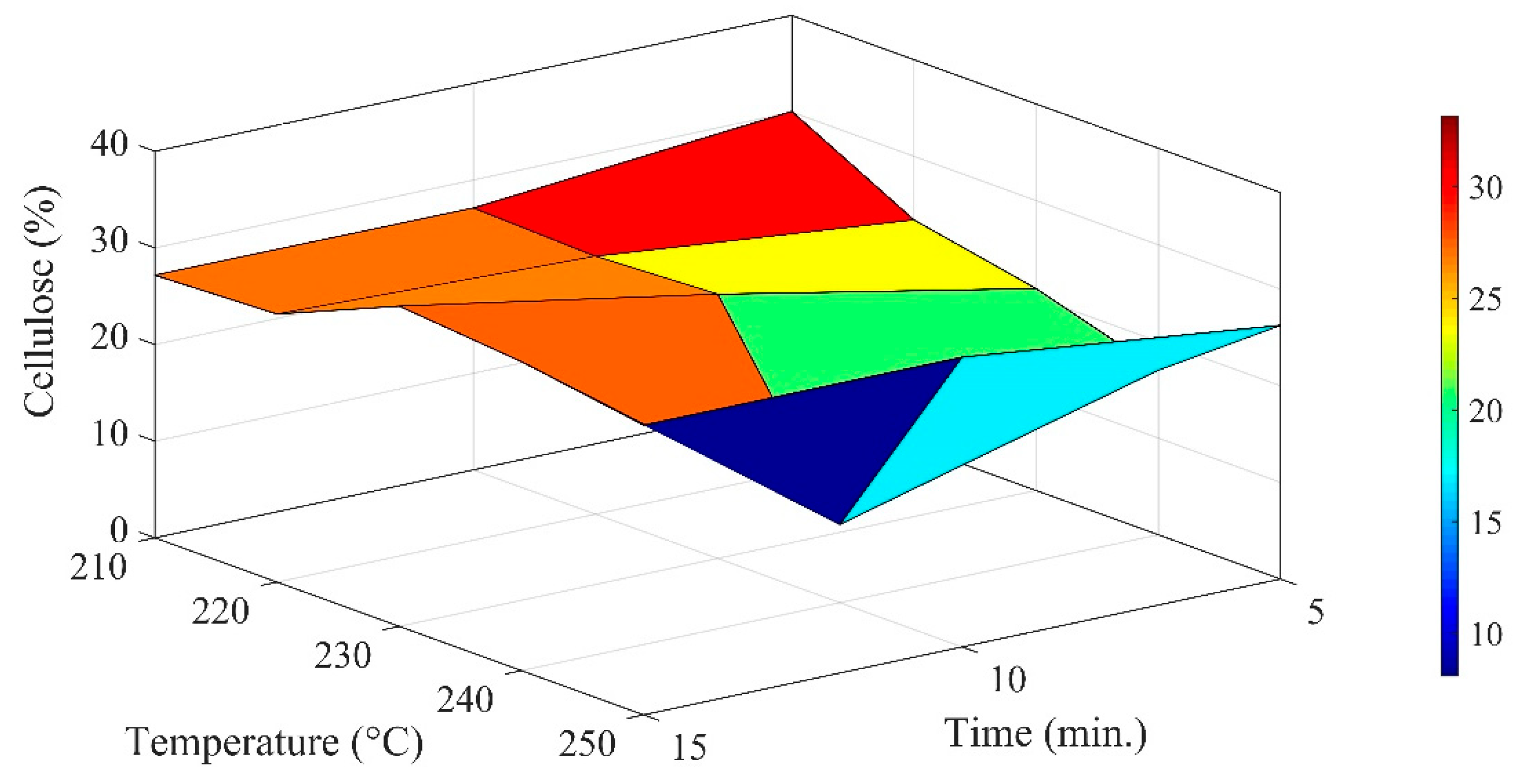
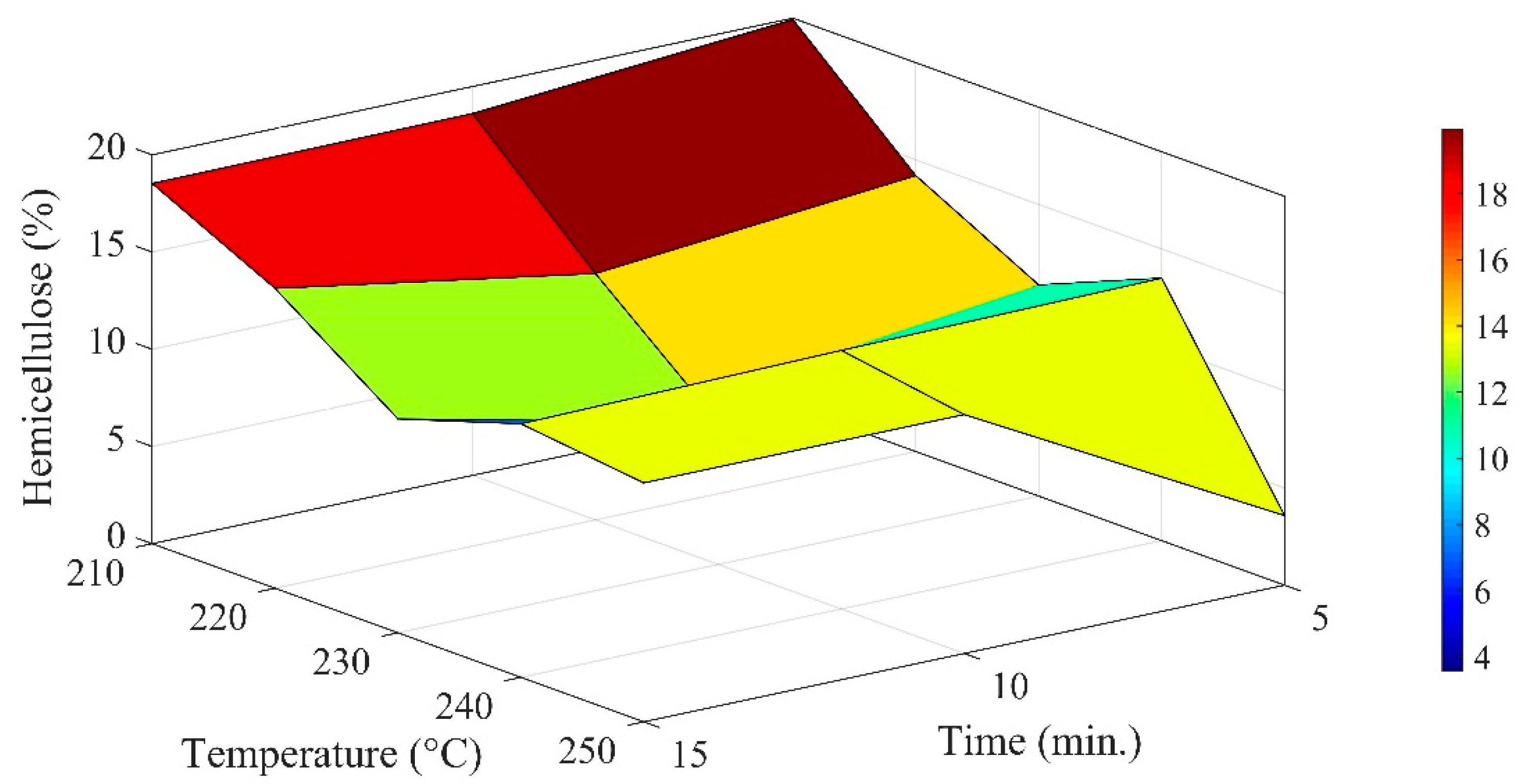
The composition of cellulose and hemicellulose after pre-treatment is graphically represented in
Figure 2 and
Figure 3. The standard uncertainty in the measurement of the cellulose fraction was in the range of ±1.33–2.57%, whereas it varied from ±1.53% to ±3.06%. The average % fractions of cellulose and hemicellulose with temperature at 5 min, 10 min, and 15 min were, respectively, 23.53%, 23.84% and 30%, and 12.41%, 12.83%, and 14.05%.
Conversely, in the context of constant temperature, the average fraction compositions of cellulose and hemicellulose were, correspondingly, 28.11%, 25.94%, 27.13%, 19.04%, and 28.74%, and 19.02%, 14.09%, 9.723%, 13.28% and 9.38% under varying temperature. As compared to the change in cellulose content for the same thermal condition, the relative percentage change in the hemicellulose fraction was lowered by 47.26%, 46.16%, and 53.15% at constant residence times of 5 min, 10 min, and 15 min. In other words, the deviation in the hemicellulose fraction would not be that much at higher residence time from that noticed in the cellulose fraction of pine cones. Similarly, at a constant temperature of 210 °C, 220 °C, 230 °C, 240 °C, and 250 °C, the corresponding recorded fall in the hemicellulose fraction was 32.34%, 45.68%, 64.15%, 30.52%, and 67.34% while comparing them with changes in the composition of cellulose at a constant temperature.
For cellulose composition, the distribution functions obtained at 5 min and 15 min were positively skewed (lies between the normal distribution and half-normal distribution), whereas the negative skewness (negative exponential distribution) was estimated at 10 min. In the same manner, uneven variation in the skewness was also seen with temperature. The distribution pattern would more likely exhibit the attribute of the symmetrical distribution at 240 °C, whereas the distribution function oscillates between exponential and half-normal distribution functions at 210 °C. In the case of 220 °C, 230 °C, and 250 °C, the characteristic pattern of probability function for the cellulose fraction falls at the intersection of the domains of the half-normal and negative distribution functions. The kurtosis estimation to determine the degree of variability in the experimental analysis showed that cellulose content would have the extremities if the torrefaction was conducted for 10 min, irrespective of temperature deviation. The distribution pattern would resemble the Laplace distribution, whereas the kurtosis (platykurtic class) obtained at 5 min and 15 min exhibits the traits of raised cosine and uniform distribution functions, respectively. In the context of temperature, the kurtosis obtained at 210 °C, 220 °C, 230 °C, 240 °C, and 250 °C remained constant, which implied outliers would not change much with temperature as compared to the residence time of torrefaction. The distribution class would be mesokurtic and the distribution would have the hybrid traits of the logistic and hyperbolic secant distribution functions. For hemicellulose, the distribution curve would be negatively skewed (negative exponential distribution) if the residence time is 5 min, whereas the distribution curves would have a positive skewness (existing between normal and half-normal distribution curves) at 10 min and 15 min of pre-processing. The kurtosis of the distribution pattern for hemicellulose was noticed to show the traits of the mesokurtic class at constant residence time. The probability distribution function varies between hyperbolic secant and logistic distribution curves. The distribution curves at 220 °C, 230 °C, 240 °C, and 250 °C were negatively skewed (negative exponential distribution) except for at 210 °C (positive exponential distribution). Similarly, the kurtosis at constant temperature will also remain constant for the dataset of hemicellulose function. The impact of time and temperature on cellulose and hemicellulose was not the same. Relatively speaking, a higher standard deviation (SD) in the cellulose and hemicellulose fraction was noticed with increasing temperature as compared to the residence time. It varied from ±2.31% to ±4.45% at constant residence time for cellulose decomposition. Conversely, the domain of variation in standard deviation at constant temperature was from ±1.38% to ±9.85%. The highest change in the SD was noticed at 240 °C, where 10 min of thermal processing recorded the maximum variation in the cellulose fraction with temperature. Concomitantly, the maximum standard deviation on the mean value of hemicellulose decomposition occurred at 5 min of thermal processing. In terms of constant temperature, thermal pre-treatment at 250 °C brought about the maximum deviation in the hemicellulose fraction with varying residence time.
The relevance of statistical information related to the datasets of cellulose and hemicellulose content shows that the probability of a reduction in the cellulose fraction would be low if the torrefaction temperature is higher at 10 min. Conversely, it would require an intermediate torrefaction temperature range to slow down the decomposition of cellulose content at 5 and 15 min. Both the parameters support the null hypothesis based on 10% of the level of significance.
3.2. The Deviation in HHV during the Thermal Pre-Treatment Process
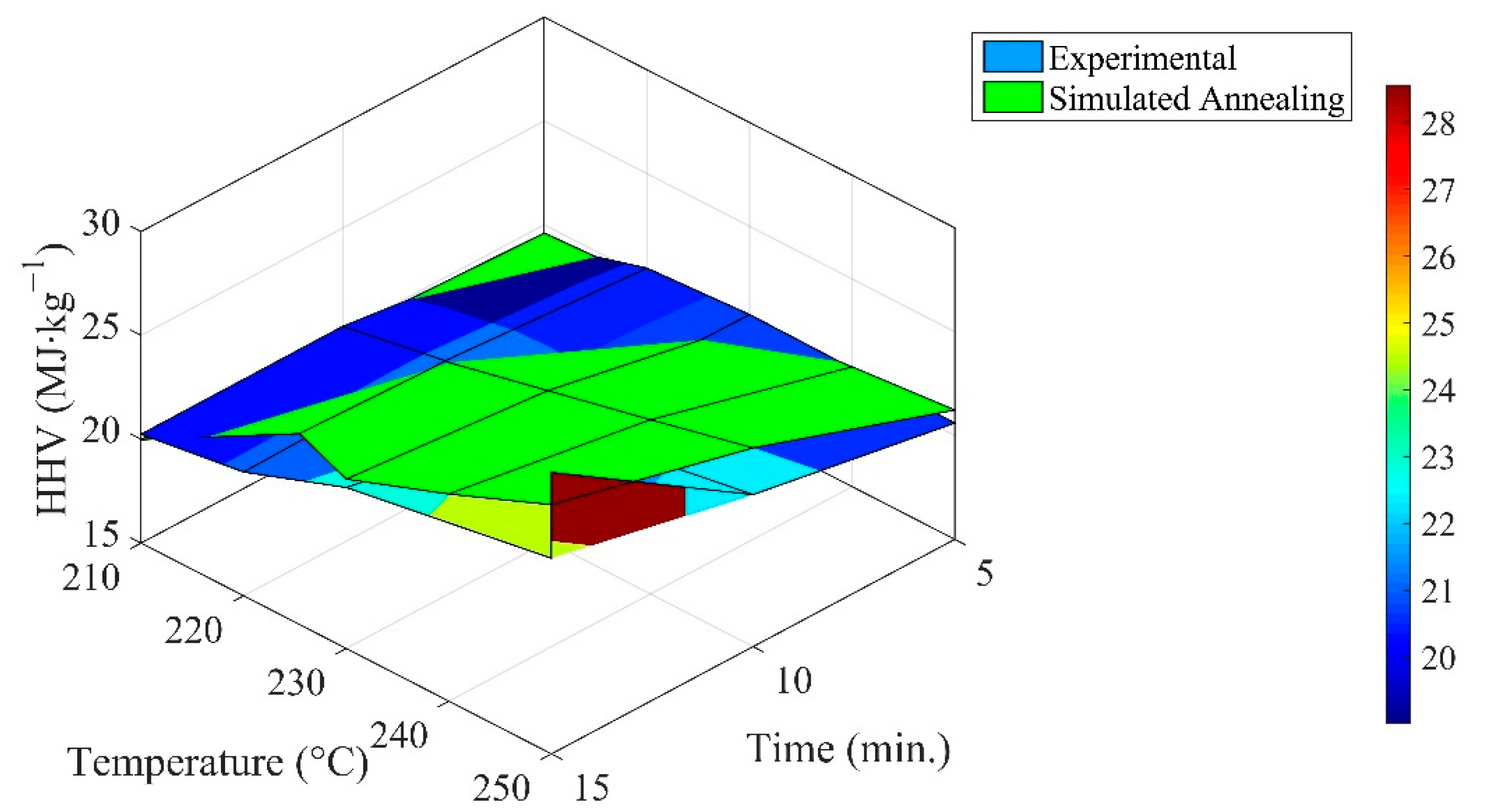
The change in
HHV with variation in residence time and torrefaction temperature is illustrated in
Figure 4. The average value of
HHV at 5 min, 10 min, and 15 min was estimated to be 20.30 MJ∙kg
−1, 21.21 MJ∙kg
−1, and 23.38 MJ∙kg
−1, respectively. Similarly, the corresponding values of
HHV were 19.84 MJ∙kg
−1, 20.85 MJ∙kg
−1, 21.44 MJ∙kg
−1, 22.20 MJ∙kg
−1, and 23.82 MJ∙kg
−1 at 210 °C, 220 °C, 230 °C, 240 °C, and 250 °C. The standard deviation in
HHV to the duration of torrefaction was the highest at 250 °C, whereas the lowest deviation from the mean value of
HHV was recorded at 220 °C. In the context of torrefaction time, the lowest and highest deviations were seen at a residence time of 5 min and 15 min, respectively. The standard uncertainty in the experimental measurement varied from ±0.33 MJ∙kg
−1 to ±1.97 MJ∙kg
−1. Statistically, the distribution function of
HHV was negatively skewed from the mean value at 210 °C and 220 °C. In the context of duration, the distribution pattern was seen to have a negative skewness only at 5 min. As compared to extremities in the dataset of
HHV obtained at 5 min, it was lowered by 88.20% and 82.85% at 10 min and 15 min, respectively. The kurtosis remained constant with variation in residence time of the torrefaction process. The probability distribution function of
HHV estimated at constant torrefaction temperature would share the trait of the super-Gaussian distribution function. Conversely, it would vary between binomial and super-Gaussian functions if the torrefaction was conducted at the constant residence time. At the alpha level of 0.1, the impact of the variation of torrefaction temperature on the
HHV rejected the null hypothesis. Based on the metaheuristic approach, the optimal solution computed at a torrefaction temperature of 300 °C with a residence time of 10 min was 30.30 MJ⸱kg
−1. The reannealing interval considered for the script was 50. The temperature function was assumed to vary exponentially with the initial annealing temperature (100 °C). The optimal solutions derived at quasistatic conditions are provided in
Table 4. It could be observed that the solution derived at 220 °C would be optimum only if the residence period is 13.62 min. The maximum value obtained within the experimental domain was noticed at 250 °C for 15 min, which is similar to the experimentally determined operating condition for the torrefaction process
3.3. Energy Requirement for the Torrefaction Process
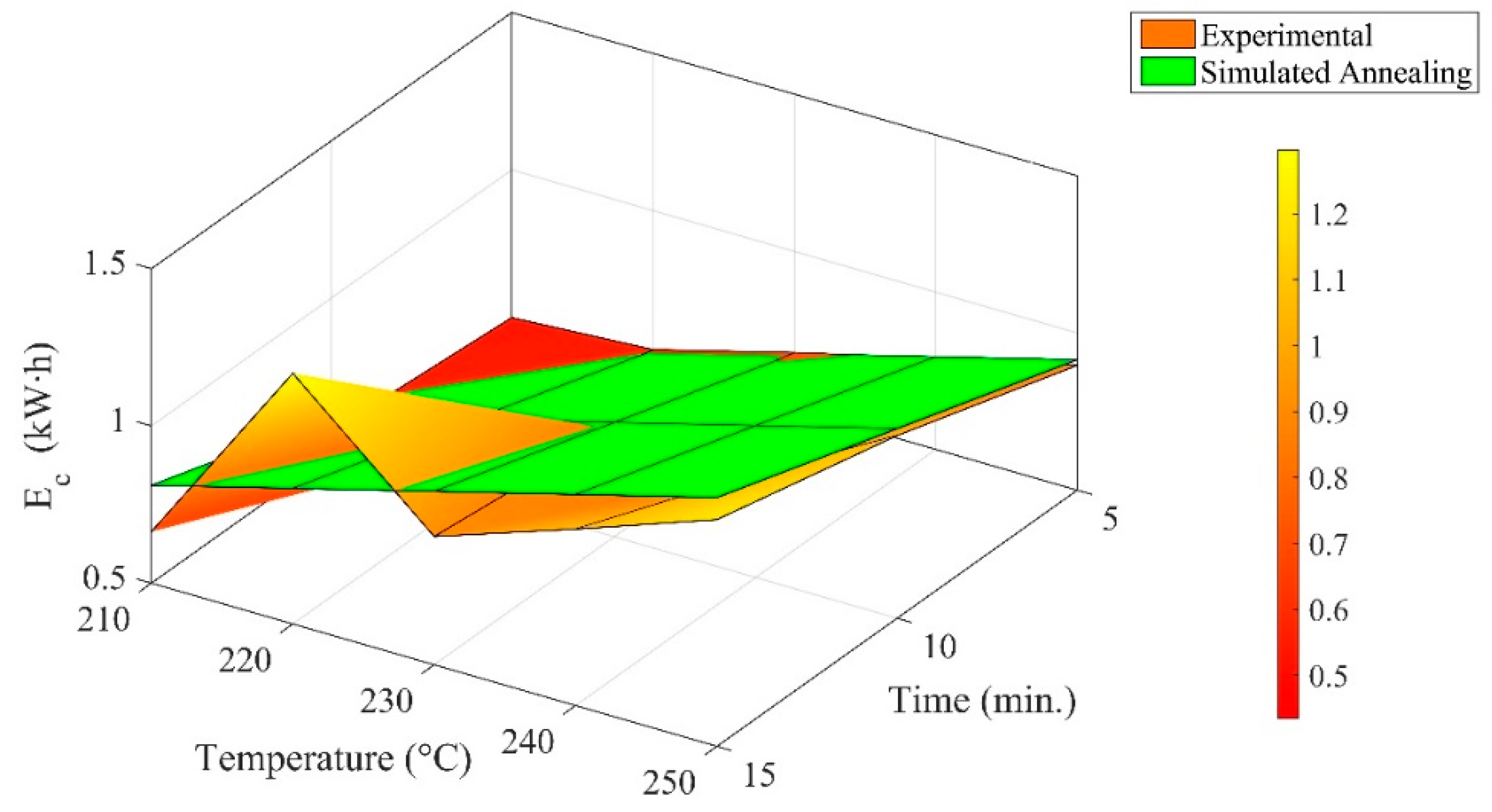
The variation in the energy consumption (
Ec) of the torrefaction unit with the change in torrefaction parameters is shown in
Figure 5. The average rise in energy consumption, as compared to the value of
Ec obtained at 210 °C, was 41.44%, 36.98%, 15.97%, and 80.63% at 220 °C, 230 °C, 240 °C, and 250 °C, respectively. In terms of residence time, a plunge of 3.01% was noticed in the
Ec with an increase in the torrefaction time by 5 min The further elevation in the duration of the torrefaction rose the
Ec by 53.76%. The perturbation in torrefaction temperature at a level of significance of 10% rejected the null hypothesis. The standard uncertainty in the measurement of the electricity consumption of the torrefaction unit was ±0.16 kW∙h (±0.03 kW⸱h to ±0.20 kW⸱h). The probability density function (PDF) of
Ec was negatively skewed about its means at 230 °C, 240 °C, and 250 °C, respectively. In the context of residence time, the distribution function was negatively skewed only at 10 min and 15 min. The distribution pattern would oscillate between a half-Gaussian and exponential function at 210 °C and 220 °C, whereas it would be the case only (lying in between normal and half-normal distribution functions) if the torrefaction was carried out for 5 min The likelihood of the existence of extremities would be high if the torrefaction was performed for 5 min. The distribution function concerning the duration of torrefaction exhibits the hybrid behaviour of the mesokurtic and platykurtic classes. The kurtosis of PDF would remain invariant (mesokurtic) with the change in the residence time of torrefaction at constant temperature. The optimal value of
Ec outside the given domain would be 0.135 kW·h for 4 min of torrefaction at 188.024 °C. The solution derived through SA is illustrated in
Table 5. The trend of variation complied with the experimental data; however, the maximum value of
Ec obtained through SA was 5.73% higher than the estimated value by the multifunction analyzer. Conversely, the global minimum was curtailed by 17.92% as compared to the minimum value of
Ec at 210 °C for 5 min.
3.4. Ash Formation during the Thermal Pre-Treatment
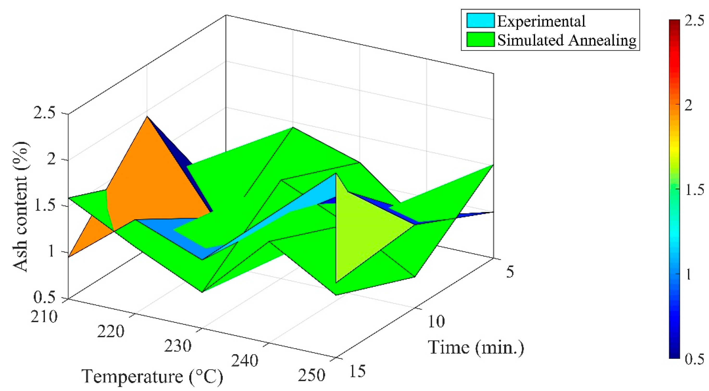
The deviation in the ash content of thermally processed pine cones with residence time and temperature is shown in
Figure 6. Through the statistical analysis, no evidence was noticed that the null hypothesis would be supported in the context of the torrefaction temperature at the level of significance of 10%. Albeit, the null hypothesis could not be refuted concerning the residence time. The standard uncertainty in the determination of the ash content varied from ±0.090% to ±0.400%. At constant temperatures of 210 °C, 220 °C, 230 °C, 240 °C, and 250 °C, the average changes in the ash content of pine cones with duration were 1.130%, 1.050%, 1.030%, 1.633%, and 1.236%, respectively. Similarly, in terms of the residence period of 5 min, 10 min, and 15 min, the corresponding average ash content was 0.730%, 1.416%, and 1.504%. The probability function of ash content was negatively skewed at 230 °C and 250 °C, whereas kurtosis would be invariant with the increasing residence period. The distribution function would fall in the mesokurtic class with constant variabilities in the dataset irrespective of the residence period. For a constant residence period, the distribution function would be positively skewed (half-Gaussian function). The outliers in the dataset would be more pronounced for a torrefaction duration of 15 min at 250 °C. The probability function of ash content would lie within the domains of platykurtic to leptokurtic classes of the distribution function.
The solution computed through the SA algorithm is provided in
Table 6. Conversely, the ash content at 220 °C (SA) rose by 0.56% while comparing with the global minimum noticed in the experimental dataset. The optimal value of ash content obtained at 340 °C for the residence time of 4 min was 0.110% (for constraints other than experimental). The global maximum solution (SA) within the experimental condition was 4.086% lower than the corresponding values calculated for the torrefied samples of pine cones. The global minimum within the experimental domain was observed at 210 °C for 5 min.
3.5. The Solid Yield Obtained after the Torrefaction Process
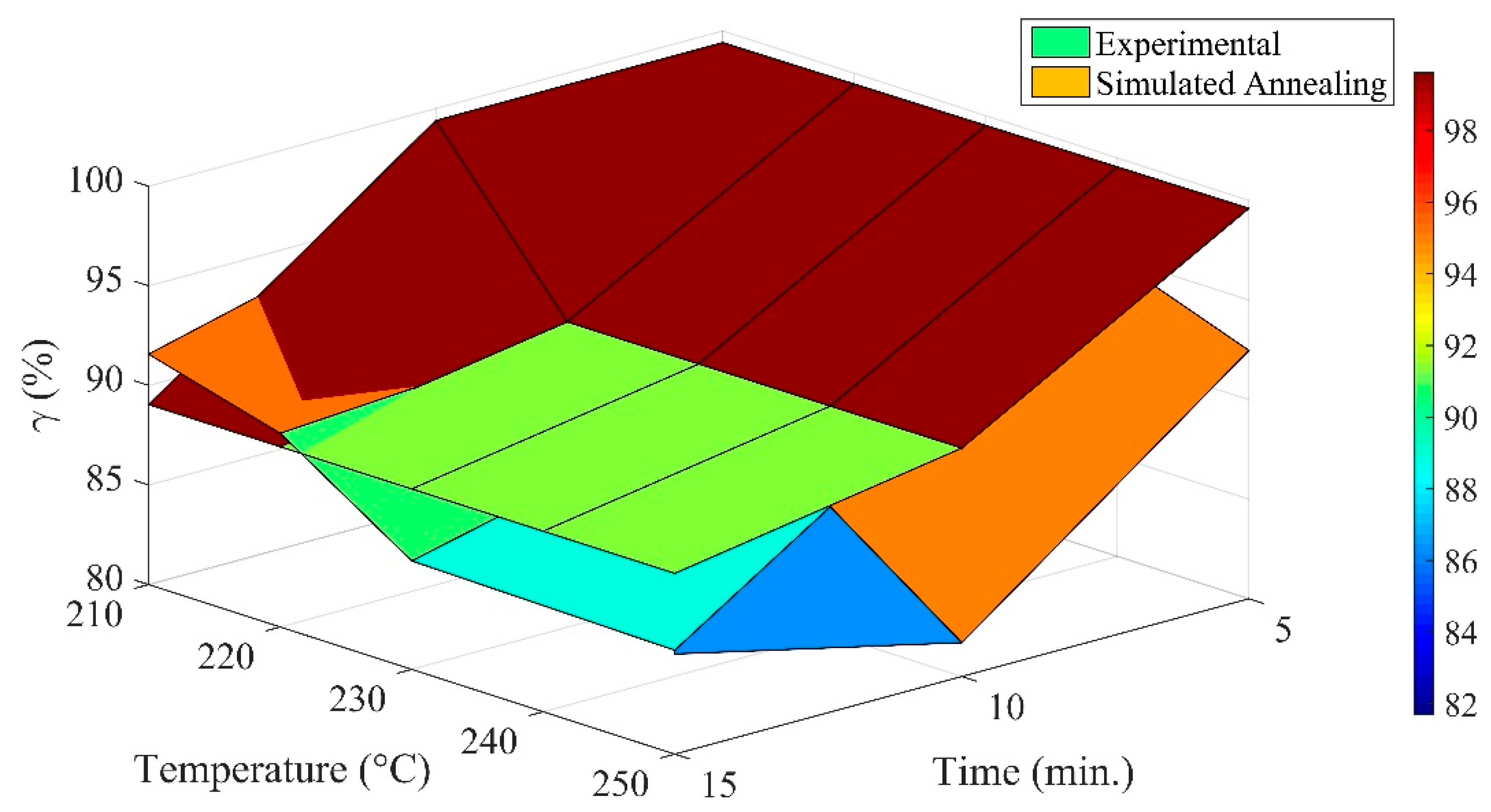
The impact of thermal pre-treatment on the solid yield of pine cones is shown in
Figure 7. The average value of solid yield (
γ) obtained at 210 °C, 220 °C, 230 °C, 240 °C, and 250 °C was, respectively, 95.20%, 92.39%, 89.85%, 88.82%, and 86.39%. The distribution function of
γ would be negatively skewed about the mean value of
γ obtained at 210 °C. The distribution trait of the probability function of
γ varied from a half-Gaussian to an exponential function for the temperature range of 220–250 °C. No deviation in kurtosis was noticed with the change in the residence time of the torrefaction process. There is no evidential proof to support the null hypothesis about the impact of temperature on the solid yield of pine cones after thermal pre-treatment. Time-related changes in the mean value of the solid yield of pine cones were highest for 5 min, whereas the lowest was encountered at 250 °C for 15 min. The probability function of solid yield at a constant residence time of 5 min would exhibit the characteristic of the normal distribution function, whereas the same would occur as a half-Gaussian function for the torrefaction period of 15 min. The negative exponential change in the PDF would be noticed for 10 min of processing of pine cones. The least variation in the solid yield would occur if the torrefaction was performed for 15 min. Based on the kurtosis values, the distribution class would vary between Bernoulli and the binomial class of distribution functions with the change in torrefaction temperature.
Detailed information on optimal solutions computed through SA is provided in
Table 7. A common solution was obtained for the maximum solid yield derived after torrefaction. The optimal solid yield would be maximized at 250 °C with a duration of 5 min. The SA exhibits a thermal lag while performing optimization at a higher temperature range for a short duration, which was not exactly the case upon estimating the values of
γ experimentally. The reason for the same is that the residence period of experimentally conducted torrefaction does not exactly comply with the algorithm of the annealing process. The global maximum solid yield estimated by SA was at operating conditions of 210 °C and 5 min.

