1. Introduction
Wind energy is a crucial clean and renewable energy source with approximately 1021 GW installed capacity throughout the whole world at the end of 2023 [
1]. Its growth rate over the past decade has been about 8% annually [
2]. Technological advancements have improved efficiency and reduced costs, making wind power an increasingly significant player in energy transition and sustainable development. However, its reliance on environmental factors leads to instability and intermittency in power output, necessitating accurate wind power prediction for reliable electricity supply and grid stability [
3,
4,
5].
With rapid progress in computer science and artificial intelligence [
6], data-driven neural network models have made significant strides in wind power prediction. Models such as Artificial Neural Network (ANN), Support Vector Machine (SVM), Random Forest (RF), and Extreme Learning Machine (ELM) have been used for wind power prediction [
7,
8,
9]. However, due to volatility and unpredictability of wind power, the accuracy of simple models may no longer meet engineering requirements [
10]. Consequently, combined prediction models have become a research focus. Reference [
11] proposes the use of SVM and an improved dragonfly algorithm to predict short-term wind power generation through a hybrid prediction model. The performance of the prediction model is enhanced by optimizing the dragonfly algorithm and selecting the optimal parameters of the SVM. Reference [
12] proposes a deep learning model that combines convolutional neural network (CNN) and long short-term memory (LSTM) networks. The model utilizes convolutional and pooling layers to extract feature information from wind power data, which is then fed into the LSTM network to capture the temporal relationships within the data and make predictions for wind power. Reference [
13] proposes an ultra-short-term wind power prediction algorithm based on LSTM combined with an extreme gradient boosting algorithm; utilizing the error reciprocal method, the prediction results of the LSTM network and the temporal convolutional neural network are weighted and summed, which improves the prediction accuracy of wind power. Reference [
14] proposes a wind power prediction algorithm based on a LSTM network model, which increases the weight of input features through an attention mechanism (ATT), thus improving the prediction accuracy of the model.
Considering the volatility and non-stationarity of actual wind power data, directly using a time series composite model to predict the original sequence may lead to inaccuracies. Therefore, processing the complex and variable wind power time series data is essential [
15]. Reference [
16] proposes using wavelet decomposition to decompose a wind speed sequence into a three-layer scale detail signal and approximate signal, and adopting the time-frequency analysis ability of wavelet decomposition to mine the original sequence information. Reference [
17] proposes using the non-recursive advantage of variational mode decomposition (VMD) to decompose the original data. Through comparison with the BP and GRU models, VMD decomposition has been shown to effectively extract the detail information of wind power sequence. Reference [
18] proposes a hybrid optimization algorithm combining VMD, maximum relevance and minimum redundancy algorithm (mRMR), LSTM, and firefly algorithm (FA). The algorithm first utilizes VMD to decompose wind power data into feature model functions, then selects the optimal feature set through mRMR, and finally optimizes LSTM parameters using FA. The prediction result is obtained by adding the prediction results of all the subsequences. Reference [
19] proposes using empirical mode decomposition (EMD) to process the original data, which improves the prediction accuracy of wind power. The results of the example show that after the EMD algorithm is decomposed, each sequence signal is relatively stable. The more stable the time series is, the more accurate the prediction result is. The EMD ensemble method can obtain multi-layer modal components and better reflect the variation characteristics of wind speed series, and has higher decomposition accuracy and prediction accuracy. However, when the number of modal components after decomposition is large, it is necessary to build a prediction model for each modal component separately. The calculation amount increases, the difficulty of data integration increases, and the prediction accuracy is reduced.
According to the existing literature review, the current data decomposition algorithms may produce many components, and simple prediction models find it difficult to make full use of all the decomposed modal component information, thus affecting the experimental results. Therefore, many studies use ATT combined with the advantages of a neural network model to process multi-data for prediction to achieve better prediction results. Based on the above literature analysis, in order to solve the problem that more modal components after EMD decomposition result in poorer experimental results, the prediction effects of simple prediction models are not ideal. Kernel principal component analysis (KPCA) is proposed to screen the modal components after EMD decomposition, reduce the dimension of input parameters, and eliminate the redundancy of different time series decomposed by EMD, then the bidirectional long short-term memory (BiLSTM) model combined with ATT is used to predict wind power. Consequently, the EMD-KPCA-BiLSTM-ATT wind power prediction model is proposed. The results of the example analysis show that compared with the six models of LSTM, BiLSTM, BiLSTM-ATT, EMD-BiLSTM, EMD-BiLSTM-ATT, and EMD-KPCA-BiLSTM, the EMD-KPCA-BiLSTM-ATT combined prediction model has obvious advantages in prediction accuracy and stability.
The main research objectives of the paper are as follows:
(1) Introducing the quartile method for handling abnormal wind power data, reducing the impact of abnormal data on the experiments and improving the accuracy of subsequent predictions.
(2) Proposing the EMD-KPCA data processing method to ensure the reduction of feature dimensions without losing the original data information, thereby improving the computational efficiency and accuracy of feature extraction.
(3) Presenting the BiLSTM-ATT prediction model, and verifying the superiority of the proposed prediction model by the examples.
The rest of the paper is organized as follows:
Section 2 introduces the methods used in wind power prediction models, including EMD, KPCA, BiLSTM, and ATT, and establishes an EMD-KPCA-BiLSTM-ATT combined model.
Section 3 analyzes the correlation coefficients between environmental factors and wind power, and processes abnormal data using the quarterback method.
Section 4 provides a detailed overview of the results obtained from each experiment and validates the effectiveness of the proposed model method.
Section 5 summarizes the paper, discusses limitations, and outlines future research directions.
2. Prediction Model Proposal
2.1. Empirical Mode Decomposition (EMD)
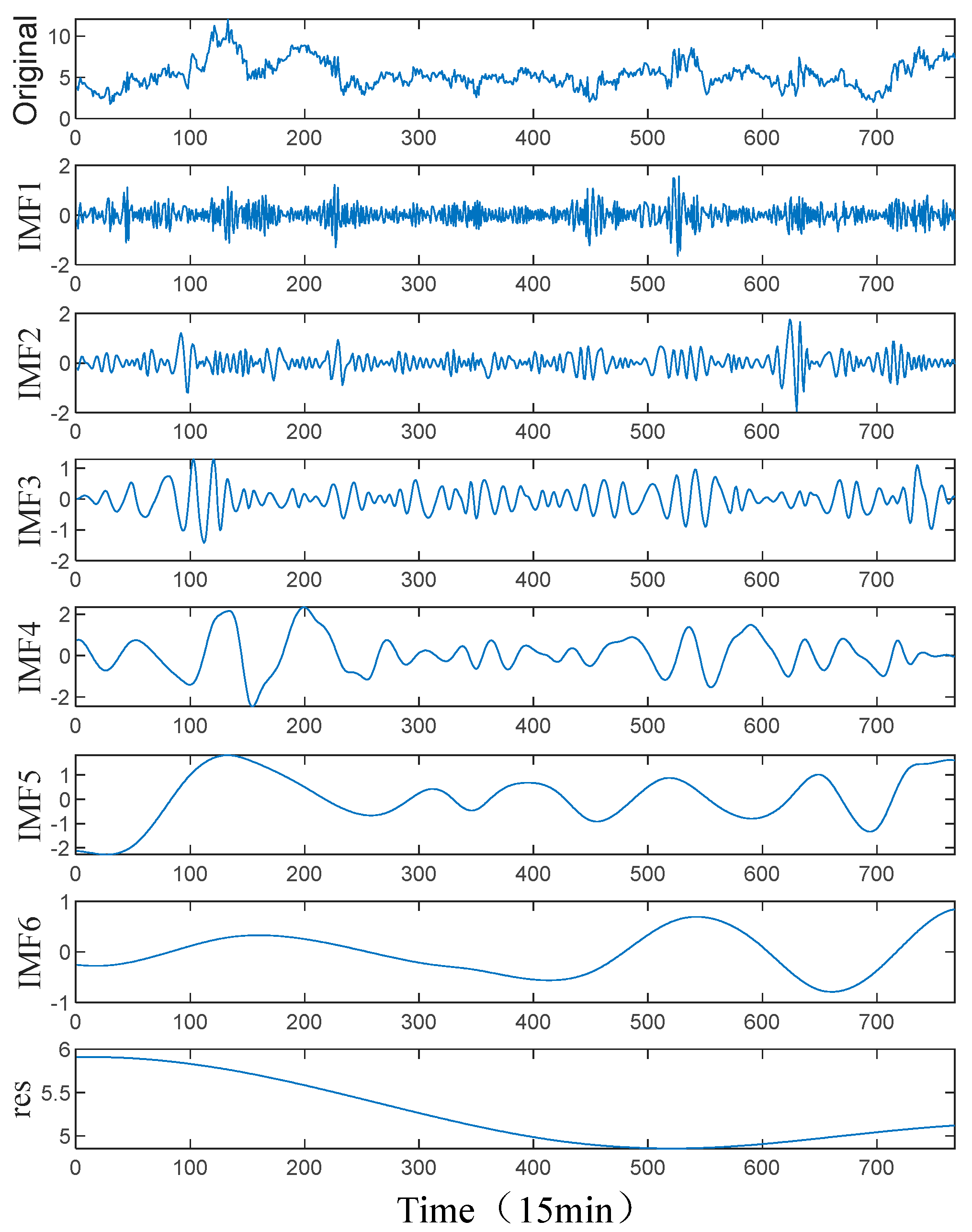
EMD is a data-based adaptive signal decomposition method, which can decompose nonlinear and non-stationary signals into several IMFs. The basic principle of the EMD method is to decompose the signal into a series of IMFs with different frequencies and amplitudes, and each IMF is a function of the local characteristics of the signal [
20]. The specific decomposition process is as follows:
(1) The extreme points of the original signal sequence are connected to form upper and lower envelopes, is the mean value of the upper and lower envelopes, and the first component is .
(2) In the second screening process, is regarded as a new sequence data, and step (1) is repeated to determine , which will be stopped when IMF conditions are met after k times. Note as the first IMF component, containing the highest frequency component in the original time series.
(3) Remove from the original sequence to yield a difference of .
(4) Take the difference as the initial time series, and repeat steps (1)~(3) to obtain n IMF components and the final residual , until is met, then terminate, where is the limiting value.
The original signal is decomposed into a series of IMFs and a residual term by the EMD method. Each IMF represents a local feature in the signal with different frequencies and amplitudes. It can adapt well to nonlinear and nonstationary signals, and has been widely used in signal processing and analysis.
2.2. Kernel Principal Component Analysis
The KPCA algorithm is an extended method of kernel function based on the PCA algorithm. Firstly, the data are mapped to the high-dimensional feature space, then the linear transformation is carried out in the high-dimensional space to achieve the effect of data discrimination and dimension reduction. Therefore, when the input data features are nonlinear, the KPCA algorithm solves the problem that the PCA algorithm can only process linear data. The specific steps are as follows:
(1) By selecting the appropriate kernel function, the original data set is mapped to the high-dimensional space to obtain the data matrix of the high-dimensional space. The multinomial kernel function is shown in Formula (1).
where
and
are original data samples;
is a mapping function that maps data to a high-dimensional feature space;
K is a high-dimensional data matrix; and
d is the highest order term.
(2) The centralized kernel matrix
Kc is calculated, which is used to modify the nuclear distance. The calculation formula is as follows:
where
is an
N by
N matrix with each element being
1/N.
(3) The eigenvalue decomposition of the kernel matrix is carried out to obtain the eigenvalues and eigenvectors.
(4) The Schmidt orthogonalization method is used to orthogonalize and unit the eigenvectors, .
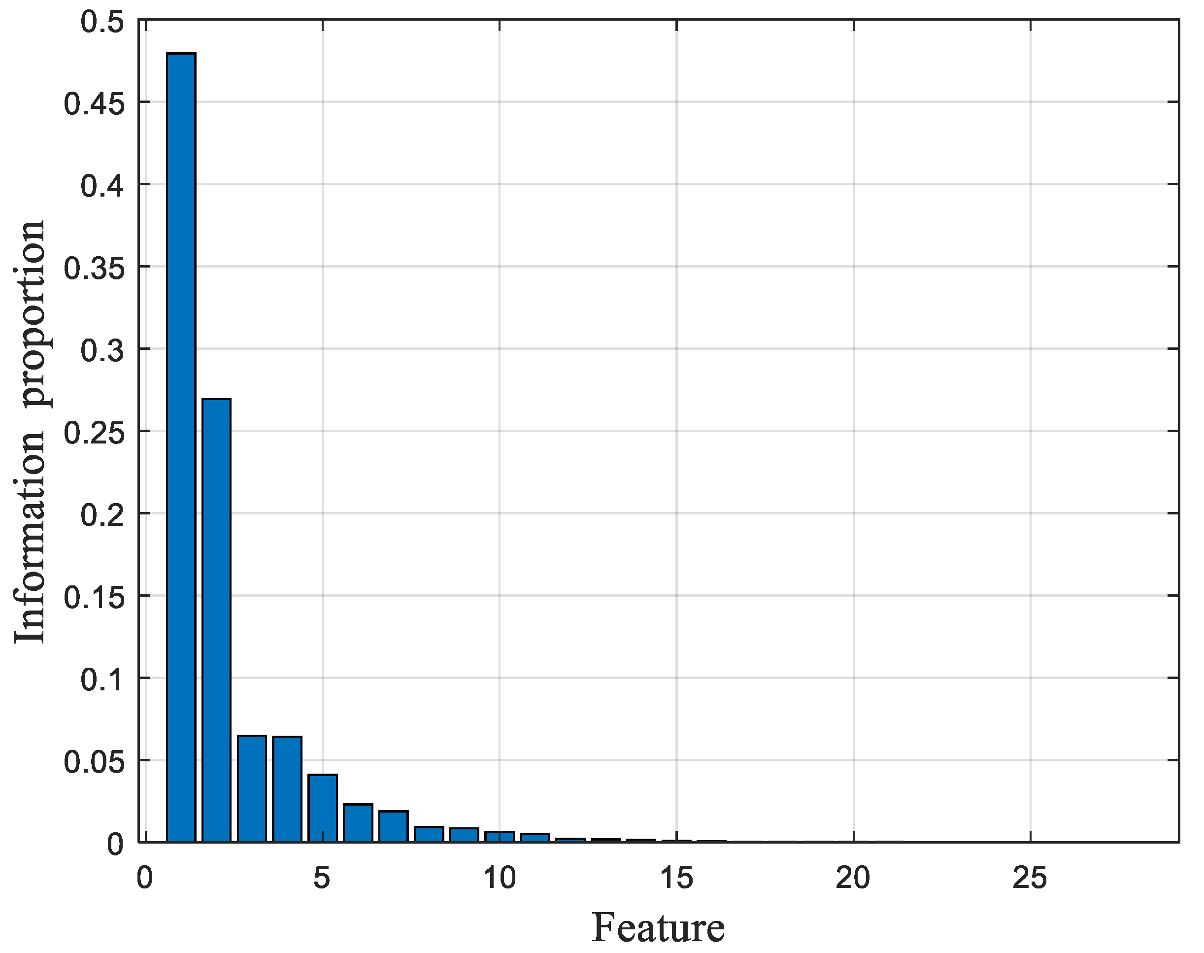
(5) The cumulative contribution rate of eigenvalue is calculated, and is selected according to the given cumulative contribution rate p. If > p, the first t principal components are used as the data after dimensionality reduction, and if < p, select again.
2.3. Attention Mechanism
ATT is a model that simulates the attention of the human brain through algorithms. The model takes advantage of the characteristics of the human brain to focus on certain important areas and pay less attention to other parts. It is widely used in natural language processing, statistical learning, and computer fields. In massive information sets, the key information is paid attention to according to the weight of attention allocation, and the influence rate of different features on the output is reasonably allocated so as to reduce the attention to non-key information and further improve the accuracy of the prediction model [
21]. The ATT formula is as follows:
where
is the attention distribution value of time
t;
u and
w are the attention weight vectors;
is a hyperbolic tangent function;
is the hidden layer state vector at time
t; e is the attention bias vector;
is the scores for attention;
is a natural exponential function; and
is the attention distribution value of time
j.
2.4. Bidirectional Long Short-Term Memory Neural Network
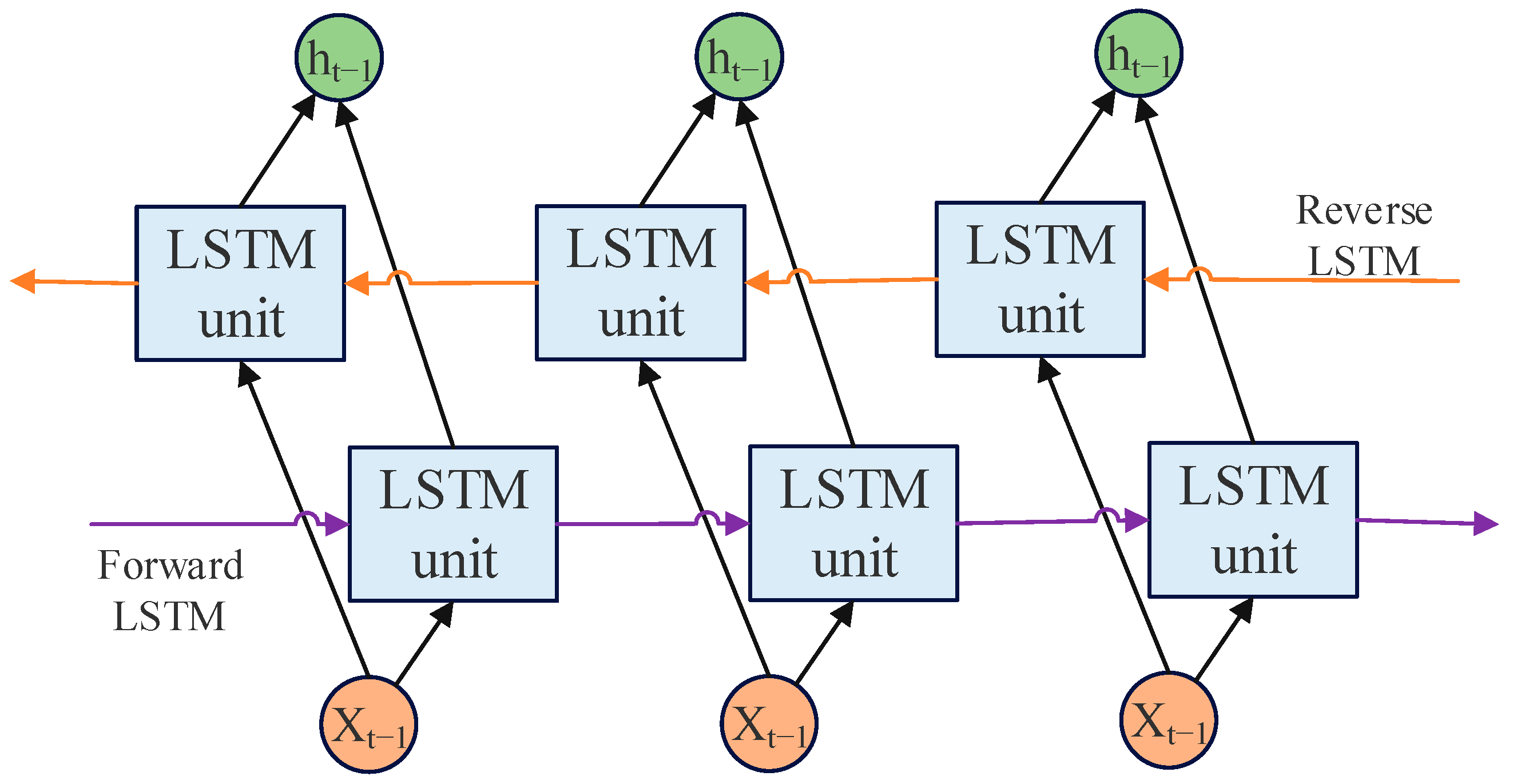
BiLSTM is composed of a layer of forward LSTM and a layer of reverse LSTM. The output of BiLSTM is determined by two layers of LSTM output, and its structure is shown in
Figure 1. Through this structure, BiLSTM can well mine the forward and reverse dependency relationship in time series, and further improve the integrity and accuracy of the network’s extraction of time series features [
22].
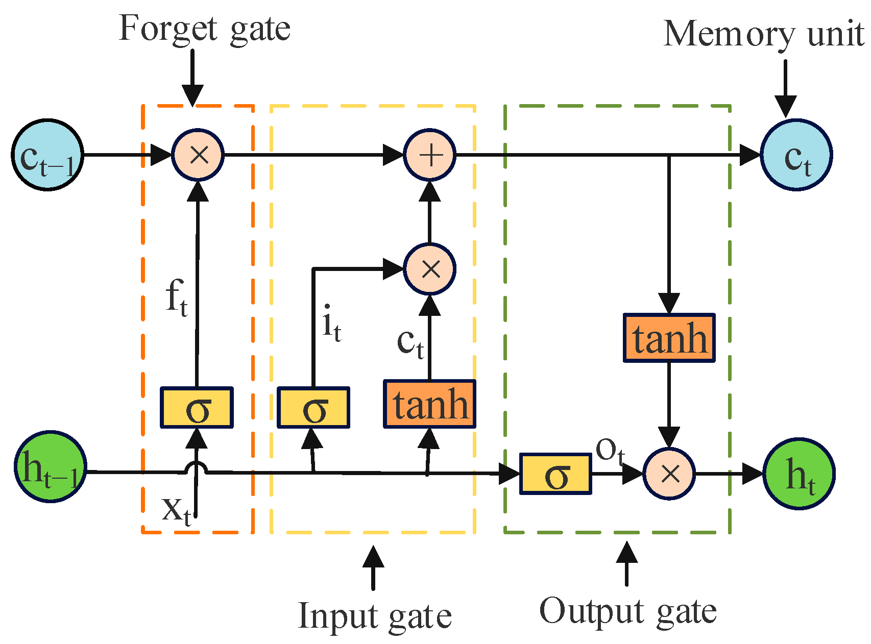
The core of BiLSTM is the LSTM unit. The LSTM is a special Recurrent Neural Network (RNN) structure, which solves the problem of gradient disappearance and gradient explosion when dealing with long sequence data experienced by traditional RNN. It can effectively capture long-term dependencies in sequence data and has achieved remarkable results in tasks such as natural language processing, speech recognition, and machine translation. The unit structure diagram of the LSTM model is shown in
Figure 2.
As can be seen from
Figure 2, the LSTM consists of the following four parts:
- (1)
Forget gate (): Determines whether the memory of the previous moment is retained or not.
- (2)
Input gate (): Determines whether the current input is added to the memory.
- (3)
Output gate (): Determines the output for the current moment.
- (4)
Memory unit (): The core component in the LSTM for storing and updating information.
The specific calculations of the forget gate, the input gate, and the output gate are shown in Formulas (5)~(10).
where σ is the activation function;
,
,
, and
are the weights corresponding to the forget gate, input gate, memory unit, and output gate, respectively;
is the output of the unit at time
t;
,
,
, and
are the corresponding gate offsets, respectively;
is the state of the candidate cell;
is the output sequence at time
t; and
is the memory unit at time
t.
In the training process, LSTM updates the network parameters through back propagation algorithm and gradient descent, so that the value of the loss function is gradually reduced and the prediction performance of the network is improved. LSTM can learn parameters to better fit the training data and suit specific tasks.
2.5. Time Attention Module
The time attention module is composed of BiLSTM and ATT, which is used as a decoder to decode the output of the feature attention module. BiLSTM is used to perform bidirectional learning on the output of the feature attention module. The ATT adaptively assigns different weights to the hidden states of the output of BiLSTM. This is determined according to the degree of influence of the history nodes of
t time steps on the current time step [
23]. Its structure is shown in Formulas (11)~(15).
where
and
are the forward and reverse hiding states of BiLSTM network at time t, respectively;
is the output of characteristic attention module;
and
are the forward and reverse weight matrices of BiLSTM network, respectively;
is the bias vector;
P is the preliminary prediction result;
is the weight matrix of all connected layers; and
is the fully connected layer bias vector.
2.6. Prediction Model of EMD-KPCA Combined with BiLSTM-ATT
Aiming at the problem of insufficient utilization of Numerical Weather Prediction (NWP) data and the unsatisfactory prediction effect of single prediction models, a wind power prediction method based on EMD-KPCA-BiLSTM-ATT model is proposed.
Firstly, the EMD-KPCA combination algorithm is used to ensure that the feature dimension is reduced without losing the original data information. This approach involves decomposing data using EMD to acquire IMFs. The IMF data are then mapped to the high-dimensional feature space using KPCA, where linear transformation is performed to achieve data identification and dimensional reduction, enabling a deeper understanding of the data structure and pattern.
Subsequently, to address the issue of the BiLSTM network’s inability to handle long-term time series dependencies, an attention module is introduced before the BiLSTM network. Using the weight that the attention module assigns to different features, the model highlights the impact of crucial components on the output while downplaying irrelevant parts. This enables the BiLSTM network to grasp the dynamic attributes of wind energy comprehensively, thereby enhancing the model’s accuracy and generalization capability.
Finally, the EMD-KPCA network integrated with the data processing module and the prediction model BiLSTM-ATT are combined for wind power prediction. The combined model is preconditioned to the data by the EMD-KPCA, which reduces the influence of external environmental factors on the prediction results. At the same time, the combination of BiLSTM and ATT can fully solve the long-term dependence problem of time series and improve the prediction accuracy.
3. Data Analysis and Prediction Process
3.1. Influencing Factor Analysis of Wind Power Generation
The experimental samples are the measured wind power data and the four environmental data factors, specifically wind speed, wind direction, air temperature, and air density, obtained by the environmental monitor corresponding to the wind farm. In order to analyze the influence of the above four factors on wind power [
24], a Pearson correlation coefficient of Formula (16) is used for calculation.
where
is the correlation coefficient;
and
are the two factor values of the
i data, respectively;
is the mean value of the environment data; and
is the mean power data.
The correlation coefficient between the environmental factors and wind power is calculated by Formula (16), as shown in
Table 1.
It can be seen from
Table 1 that the wind speed has the greatest impact on power output, the correlation coefficient between the wind direction and the air density is negatively correlated, and the air temperature has a relatively small impact.
3.2. Processing of Abnormal Data
The collection of wind power data is affected by many factors such as wind speed, wind direction, air temperature, and air density. These factors may lead to abnormal data which generate a decrease in power prediction accuracy. Therefore, before training the wind power prediction model, it is necessary to process the abnormal data to improve the quality of the data [
25].
Compared to traditional statistical methods and clustering algorithms, the quartile method is a commonly used data cleaning technique that is robust, intuitive, and easy to calculate. By identifying and processing outliers, this method can enhance data accuracy, maintain data distribution stability, and improve the reliability of data analysis. Choosing the quartile method for data cleaning can effectively enhance data quality and provide better support for subsequent data analysis and application.
The data processing method is to arrange the data set in order of size and divide it into four equal scores, namely, the first quantile , the median , the third quantile and the interquartile distance , with each equal fraction containing 25% of the data. Use the quartile method to clean abnormal data, the specific process is as follows:
(1) Arrange a set of data in ascending order to obtain the sorted data sample .
(2) Calculate the median
.
(3) Calculate the first quantile and the third quantile . When , the original data X is divided into two parts by the median . The median of the two parts is calculated according to Formula (18), that is, and , and < .
When
, then:
When
., then:
The interquartile distance
is determined by:
According to the interquartile distance, the normal wind data range can be determined as:
where
and
are the upper and lower limits of normal data respectively.
Data outside the upper and lower limits of
W1 and
W2 are considered as abnormal data and need to be cleaned. At the same time, the cleaned data are filled using the linear interpolation method. The calculation formula is as follows:
where
is the wind power data at time
i.
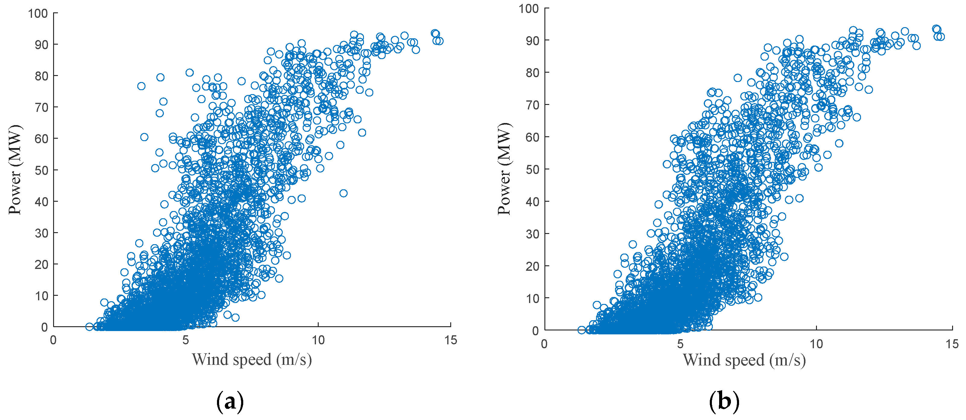
Taking wind speed and power data as an example, the scatter diagram of wind power before and after cleaning is shown in
Figure 3.
It can be seen from
Figure 3 that the use of the quartile algorithm effectively eliminates the scattered abnormal data in the original data, and the cleaned scatter plot is closer to the standard wind speed-power scatter.
3.3. Evaluation Indexes
In order to evaluate the prediction results of the model, Mean Absolute Error (MAE), Root Mean Square Error (RMSE), Mean Absolute Percentage Error (MAPE) and R-Squared (R
2) were selected as evaluation indexes [
26]. Each evaluation index is calculated as follows:
where
m is the number of test sample;
is the real output power of wind power; and
and
are the prediction and average values of wind power output, respectively.
3.4. Prediction Process
In order to improve the prediction accuracy, a combined prediction model was constructed using EMD-KPCA algorithm and BiLSTM-ATT network. The prediction process is shown in
Figure 4, and the specific steps are as follows:
(1) Abnormal data process: The original data are screened and filled by the quartile and linear interpolation methods.
(2) Empirical mode decomposition: EMD is used to decompose the data to obtain a series of IMF components and residual components.
(3) Kernel principal component analysis: The KPCA algorithm is used to calculate the contribution rate of each component for dimensionality reduction, and the feature data after dimensionality reduction will form a new data set.
(4) Data normalization process: The normalized data set is divided into a training set and a test set.
(5) Determination of optimal parameters of the proposed model: The training set data are used to train the BiLSTM-ATT combined prediction model, and the prediction results are compared to determine the hyperparameters to achieve the target accuracy.
(6) Wind power prediction: Using the test set data to test the prediction model, the wind power to be predicted is obtained, and the prediction effect is evaluated.
5. Conclusions
In order to make full use of historical data, improve the accuracy of wind power prediction, and meet the high-precision requirements of power system for wind power prediction, a short-term wind power prediction method based on the EMD-KPCA-BiLSTM-ATT model is proposed. First, the abnormal data were processed using the quartile method. Subsequently, the wind power data were analyzed and processed by EMD decomposition and KPCA selection of key components. Following this, the BiLSTM-ATT combined prediction model was utilized to predict the examples. Finally, seven methods were employed to predict the examples, and the results were compared. The effectiveness of the prediction method is verified by the example, and the following conclusions are obtained:
(1) When dealing with multivariate input data, the combination of EMD and KPCA is used to decompose input data and screen main feature sequences, which can fully exploit the information features and improve the prediction accuracy of the model.
(2) The prediction effect of the BiLSTM-ATT model is better than that of the LSTM model, and the LSTM model cannot process the hidden features in the data. The ATT can capture crucial information within the input sequence during prediction, and better focus on the output power related part of the input data, while BiLSTM is good at learning the long dependence characteristics in the data. Therefore, the combination of the two algorithms can improve the performance, interpretability and adaptability of the model, so that the model can better deal with complex input data.
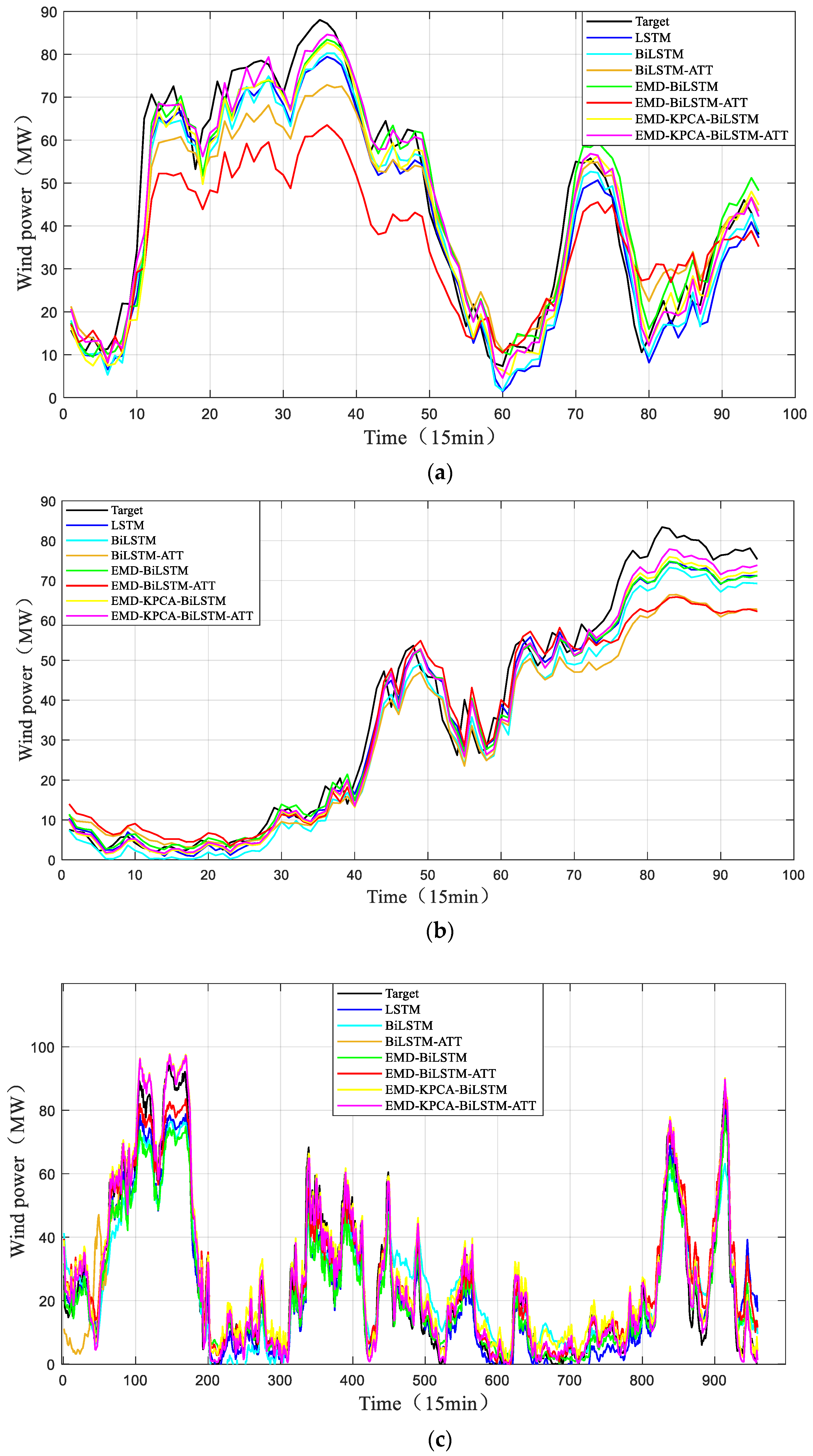
(3) Compared with LSTM, BiLSTM, BiLSTM-ATT, EMD-BiLSTM, EMD-BiLSTM-ATT, and EMD-KPCA-BiLSTM models, the EMD-KPCA-BiLSTM-ATT model has smaller prediction error and higher accuracy, which verifies the effectiveness of the model in short-term wind power prediction for wind farms and provides a new idea for improving wind power prediction accuracy.
After analyzing the existing research, there are still some issues with power prediction. Firstly, existing wind power point prediction models are often influenced by changing weather conditions, leading to low prediction accuracy. Secondly, these models often only consider partial factors, lacking comprehensiveness and integration. Future research directions may include taking all aspects of power prediction into account, extending the prediction time span or adopting power range prediction, and exploring more complex machine learning algorithms or deep learning models to further improve prediction accuracy and stability.
