Article

Short-Term Wind Power Prediction Based on a Variational Mode Decomposition–BiTCN–Psformer Hybrid Model

1
School of Electrical and Information Engineering, Yunnan Minzu University, Kunming 650504, China
2
Yunnan Key Laboratory of Unmanned Autonomous System, Kunming 650504, China
3
Lancang-Mekong International Vocational Institute, Yunnan Minzu University, Kunming 650504, China
*
Author to whom correspondence should be addressed.
Energies 2024, 17(16), 4089; https://doi.org/10.3390/en17164089
Submission received: 17 June 2024 / Revised: 10 August 2024 / Accepted: 15 August 2024 / Published: 17 August 2024
(This article belongs to the Special Issue Advances in AI Methods for Wind Power Forecasting and Monitoring)

Abstract

:
Precise wind power forecasting is essential for the successful integration of wind power into the power grid and for mitigating the potential effects of wind power on the power system. To enhance the precision of predictions, a hybrid VMD-BiTCN-Psformer model was devised. Firstly, VMD divided the original sequence into several data components with varying time scales. Furthermore, the BiTCN network was utilized to extract the sequence features. These features, along with the climate features, were then input into the positional encoding and ProbSparse self-attention improved Transformer model. The outputs of these models were combined to obtain the ultimate wind power prediction results. For the prediction of the wind power in Fujian Province on April 26, four additional models were developed for comparison with the VMD-BiTCN-Psformer model. The VMD-BiTCN-Psformer model demonstrated the greatest level of forecast accuracy among all the models. The R2 increased by 22.27%, 12.38%, 8.93%, and 2.59%, respectively.

1. Introduction

In 2020, China put forward the goal of “reaching peak carbon by 2030 and achieving carbon neutrality by 2060” [1]. Global carbon dioxide emissions from energy combustion hit a historic peak of 36.8 billion tons in 2022. Hence, wind energy, which embodies the latest advancements in energy generation, has emerged as a pivotal area of investigation in multiple nations [2]. Nevertheless, meteorological factors in the atmosphere change rapidly, causing transient or short-term fluctuations in wind power generation. This poses a challenge to the optimum scheduling and safe operation of the power system [3,4]. By improving the accuracy of wind power prediction, the grid scheduling department can rationally arrange the power generation plan and improve the economy of grid operation.
With the development of Artificial Intelligence (AI) [5], machine learning models [6] and deep learning models have been widely used in wind power prediction and are gradually replacing previous methods. Reference [7] presents a distinctive hybrid forecasting model that integrates Long Short-Term Memory (LSTM) with Gauss, Moret, Ricker, and Shannon for power forecasting. This integration enhances the utilization of deep learning by tackling issues like gradient vanishing and nonlinear mapping through the use of wavelet transforms, thus enhancing the precision of wind power prediction. Reference [8] introduces a novel framework designed to improve the accuracy of predicting wind power generation in 5 min intervals. The system incorporates signal decomposition and heuristic techniques, known as CEMOLS, to optimize the parameters of neural networks. Reference [9] introduces the AMC-LSTM model designed for wind power forecasting. It includes an Attention Mechanism to dynamically assign weights to physical attribute data, utilizes Convolutional Neural Networks (CNN) to extract short-term features, and applies LSTM to capture long-term trends. In reference [10], Three types of Deep Neural Networks (DNNs) were used for the experiment and the best result was achieved with the Gated Recurrent Unit (GRU) network. Reference [11] introduces a novel spatiotemporal directed graph convolution neural network and verify the superiority of the proposed model in spatiotemporal correlation representation. Reference [12] combines point prediction and probability density prediction, and the results show accurate prediction in extreme weather. The literature outlined above demonstrates that the accuracy of the prediction model can be significantly enhanced by the utilization of various model combinations.
The Transformer is a highly effective deep learning model architecture that demonstrates strong performance when applied to continuous data. It is becoming increasingly popular in the field of wind power prediction. Reference [13] utilizes transformer neural networks that incorporate a multi-head attention mechanism to effectively capture successive dependencies, irrespective of their distance. The reference [14] investigates the application of Transformer-based architectures: Informer, LogSparse Transformer, and Autoformer for the first time. The study carried out in [15] introduces a novel deep neural network structure based on transformers that incorporates wavelet transform to predict wind speed and wind energy generation up to 6 h ahead. The author of [16] introduces a wind power forecasting model that integrates LSTM to capture the temporal dynamics of weather data and a Vision Transformer (ViT) to construct connections between extracted characteristics and desired outputs using multi-headed self-attention methods. However, the conventional Transformer model encounters the issue of significant time complexity when handling long sequential data, which can be resolved by using Probsparse self-attention. The ProbSparse self-attention mechanism achieves a time complexity and memory consumption of O (LlogL), which presents a significant enhancement compared to the self-attention mechanism in the conventional Transformer model [17]. We utilized the Probsparse self-attention to enhance the original self-attention mechanism of the Transformer, which we refer to as the Psformer.
The Temporal Convolutional Network (TCN) utilizes convolutional operations to extract and acquire features from time series data. It has demonstrated a strong performance in many applications, including time series prediction and classification. Reference [18] employs a deep clustering model based on the Categorical Generative Adversarial Network (CGAN) for precise classification. Additionally, they enhance the TCN by integrating a gating mechanism within its activation function. In reference [19], an enhanced Temporal Convolutional Network (MITCN) is devised for predicting multi-step time series. They have incorporated the quadratic spline quantile function (QSQF) to facilitate probabilistic forecasting. Recently we have found that bi-directional neural networks are gaining popularity due to the fact that they can capture contextual information about both past and future states, which makes it possible to accurately model and predict sequences with long-term dependencies. To address the issue of offshore wind power generation being affected by extreme weather conditions, reference [20] introduces a new prediction method that merges convolution and attention mechanisms. The approach integrates a bidirectional long short-term memory (BiLSTM) network with an attention mechanism (AM). It is proved that the mean square error of this model is much lower than that of LSTM without bidirectional structure. In [21], BiLSTM’s bidirectional capability was also used to extract deep correlation in data to analyze wind power data. Reference [22] proposed a model based on the XGBoost algorithm combining financial technical indicators, The model has high prediction accuracy and speed. Reference [23] presents a hybrid model that combines BiTCN and BiLSTM with an attention mechanism; the attention mechanism improves the model’s capacity to concentrate on significant characteristics. From the recent literature, it can be seen that neural networks with forward and reverse processes are becoming more widely used than traditional neural networks.
Data decomposition is a highly successful technique for extracting the underlying patterns in data, thereby lowering the complexity of training prediction models and improving their accuracy. The Wavelet Packet Transform (WPT) [24] uses a collection of orthogonal and rapidly decaying wavelet function bases to accurately fit signals. Ensemble Empirical Mode Decomposition (EEMD) [25] is an enhanced version of Empirical Mode Decomposition (EMD) [26]. EEMD improves EMD by introducing white noise into the signal to fill in missing scales. This technique has demonstrated excellent performance in signal decomposition. Variational Mode Decomposition (VMD) [27] is an algorithm that iteratively searches for the optimal solution of a variational model to identify the center frequency and bandwidth of each component. This algorithm is a completely non-recursive model. The experimental findings from reference [28] demonstrate that the decomposition impact of VMD is more pronounced in power prediction compared to EMD.
According to the aforementioned research, the majority of studies focus solely on enhancing prediction accuracy through the integration of one or two models. There is a scarcity of research that combines signal decomposition, BiTCN extraction features, and the Transformer model. Therefore, we propose a novel hybrid prediction model named VMD-BiTCN-Psformer, which offers the following key contributions:
  • Through VMD, the original signal is decomposed as a whole into other component signals. The decomposition process is carried out on the features of specific significance and can yield a greater amount of comprehensive information and structure within the signal.
  • The concept of position encoding is utilized to extract the hidden aspects of multi-scale temporal seasonal information, which are then merged with position encoding.
  • BiTCN was introduced to extract features of near-time segments of observation points, expand the scope from which the model may acquire information and generate predictions, and adjust the connection structure of the self-attention mechanism and BiTCN output data.
  • The ProbSparse self-attention is introduced, and the Psformer model is designed to integrate the characteristics of significant time points into the self-attention mechanism, resulting in enhanced forecast accuracy of wind power and reduced computational complexity.

2. Materials and Methods

2.1. Decomposition of Wind Power Using VMD

To address the unpredictable, variable, and ever-changing characteristics of wind power time series, decomposition techniques are often employed to reveal their inherent features and enhance the precision of wind power forecasting. Variational Mode Decomposition (VMD) was proposed by Dragomiretskiy et al. in 2014 [29]. The model uses a collection of modes and their respective center frequencies in order to accurately reproduce the input signal as a whole. Furthermore, each mode is smoothly demodulated to the baseband. The alternate direction multiplier approach is employed to optimize the variational model effectively, thereby enhancing the model’s robustness to sampling noise.
The goal is to minimize the total bandwidth of each modal component while ensuring that the sum of all modal functions after decomposition is identical to the original signal before decomposition. Equation (1) is a problem with constraints. To solve this problem, we converted it into an unconstrained variational problem, as depicted in Equation (2), by incorporating Lagrange multipliers and second-order penalty factors.
min ν k , ω k k t δ t + j π t ν k ( t ) e j ω k t 2 s . t . k ν k = s ( t )
L ν k , ω k , τ = α k t δ t + j π t ν k ( t ) e j ω k t 2 + s t k ν k t 2 + τ t , s t k ν k t
where δ t is the Dirac function, ν k t is the k-th modal component, ω k ( t ) is the k-th center frequency, s ( t ) is the original wind power, ∗ denotes convolution.
The saddle point of Equation (1) is solved by iteratively updating the solution, employing the alternating direction multiplier method described in Equations (3)–(5).
ν ^ k n + 1 ω = s ^ ω i k ν ^ i ω + τ ^ ω / 2 1 + 2 α ω ω k 2
ω k n + 1 = 0 ω ν k n + 1 ω 2 d ω 0 ν k n + 1 ω 2 d ω
τ ^ n + 1 ω = τ ^ n ω + τ s ^ ω ν ^ k n + 1 ω
where s ^ ω , ν ^ k ω , and τ ^ ω are the Fourier transformed form of s ( t ) , ν k t , and ω k ( t ) , n is the number of iterations.
The algorithm stops when Equation (6) is satisfied, otherwise, it continues updating the values.
k ν ^ k n + 1 ν ^ k n 2 2 / ν ^ k n 2 2 < ε ( ε > 0 )

2.2. Original Transformer’s Multi-Head Self-Attention

The Transformer self-attention equation is:
A ( Q , K , V ) = Softmax ( Q K T d ) V
where A (.) represents the function of attention, Q, K, V represents the query, key, and value matrix, respectively. Softmax represents the fixed normalized exponential function, and d is the dimension.
The utilization of the multi-head self-attention mechanism enhances the capacity of the model to convey information effectively. Equation (8) illustrates the functional structure of the d-th self-attention in the multi-head self-attention mechanism.
M ( Q , K , V ) = Concat ( H 1 , H 2 , , H d ) W o
H g = A ( Q W g Q , K W g K , V W g V )
where M (.) represents multi-head self-attention function, Concat(.) represents the concatenation function, H g represents the g-th self-attention function, W o represents linear mapping matrix of the mechanism, Q W g Q , K W g K , and V W g V represent the linear mapping matrix of Q, K, and V, W represents the weight matrix.

2.3. Original Transformer’s Positional Encoding

Transformer adopts a parallel structural framework that is unable to capture temporal and positional features. To compensate for this shortcoming, Transformer neural networks usually use absolute position encoding to obtain positional information from the data, as seen in Equations (10) and (11).
P ( l , 2 k ) = sin ( l 1000 2 k d model )
P ( l , 2 k + 1 ) = cos ( l 1000 2 k d model )
where P shows the bit encoding, l is the sequential position corresponding to the encoded data, d model is the dimension, and k is an integer value between 0~0.5 d model − 1.

3. Model of VMD-BiTCN-Psformer

3.1. Improvement of Transformer’s Positional Encoding

For time-series data, time-hidden features are essential in addition to location information. Therefore, we improved the original location coding of Transformer by incorporating temporal and seasonal information encoding. Based on the concept of positional encoding, time features are processed to extract global time features from different timestamps. The dimensions of time encoding, hourly encoding, daily encoding, and monthly encoding are normalized and then merged.
In Figure 1, un is the projection of wind farm data series, pn is absolute positional encoding, tn, hr, de, and mw represents temporal and seasonal information encoding data in different time dimensions.
After splicing the three parts, cn is obtained, and the equation for this is:
c i t = α μ i t + P i t + z E i , z t
where c i t represents the i-th column data for the t-th sequence input, u i t is the normalized vector of the i-th column data for the t-th sequence input, P i t is the absolute positional encoding of the i-th column data for the t-th sequence input vector quantity, E i , z t is the encoding vector for the i-th column data input for the t-th sequence normalized according to the z time dimension, z E i , z t represents the data after normalization processing of time, hour, day and month encoding, and z is the number of time dimensions.

3.2. BiTCN

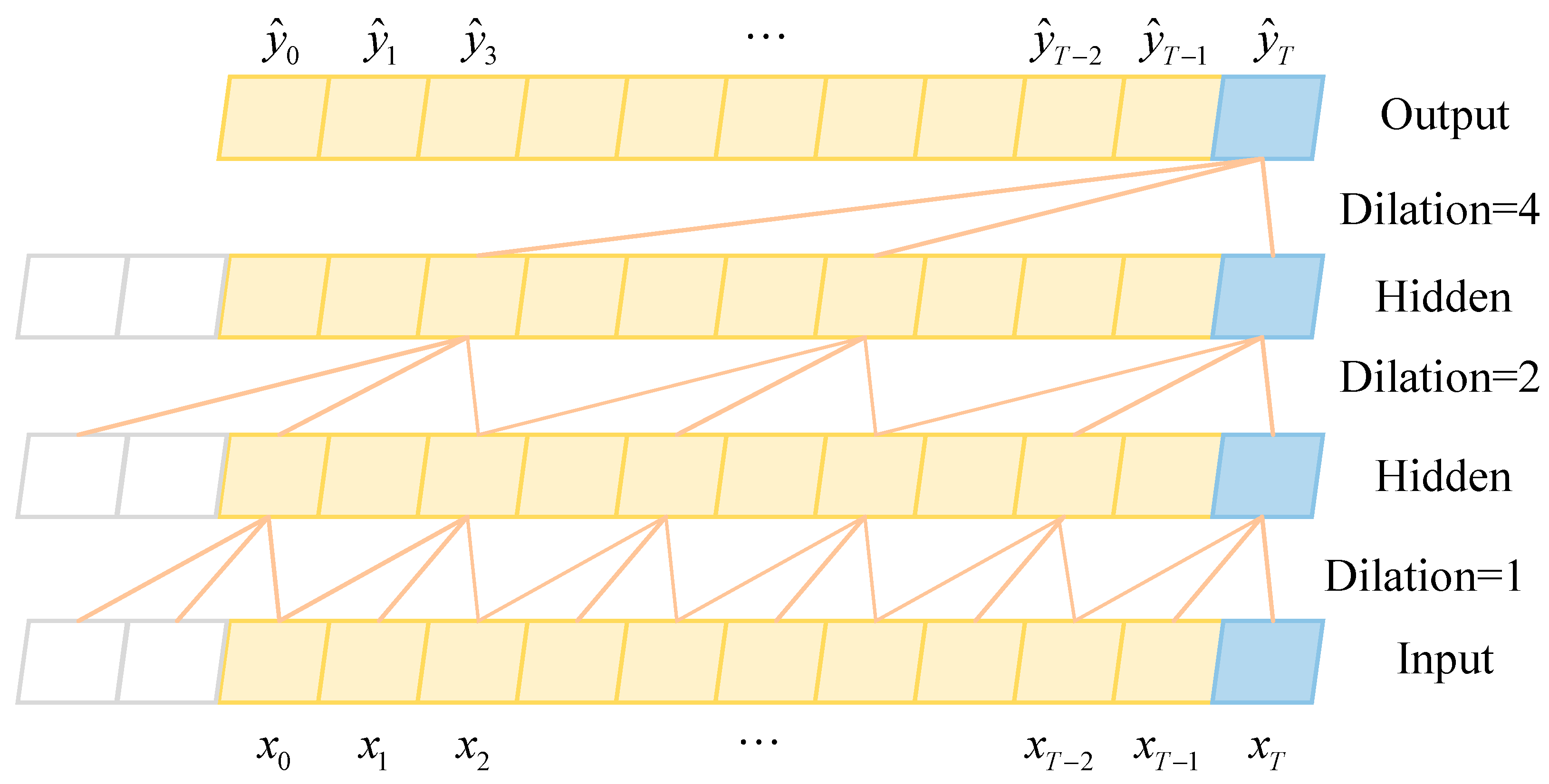
TCN is a model that combines the benefits of causal convolution and expansive convolution, building upon the CNN paradigm. Figure 2 shows the structural diagram of TCN.
Prioritizing the prevention of information leakage is crucial for long-term data prediction challenges. In contrast to convolution in a CNN, causal convolution is a unidirectional structure in which the features extracted at time t are solely influenced by the values of the current and previous moments, and the original data after time t cannot be used. By utilizing dilated convolution in TCN, the model can attain a larger receptive field with a reduced number of layers. This is possible because the input can be sampled at intervals during convolution, leading to an exponential increase in the size of the receptive field as more layers are added. Thus, TCN can effectively capture long-range dependencies and temporal patterns in the input data while reducing computational complexity. The equation for TCN causal unfolding convolution is:
H ( t ) = i = 0 k 1 h ( s ) x t d m s
where H ( t ) represents the t-th output of TCN, k is the kernel size, h ( s ) is the s element in the convolution kernel, x t d m s is the input, dm is the expansion factor.
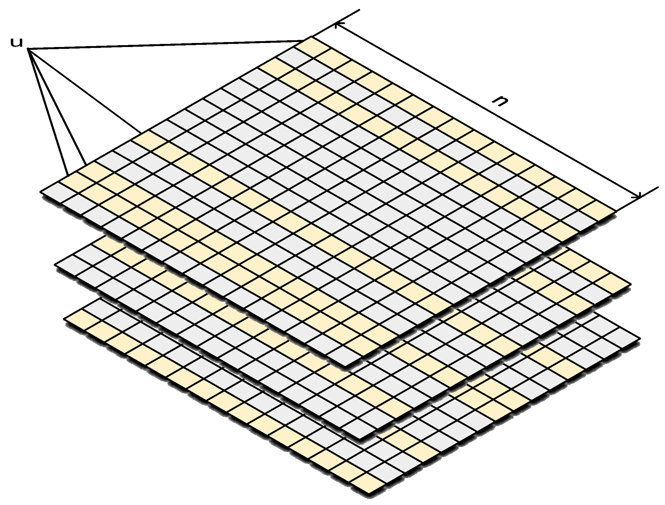
TCN exclusively focuses on the forward convolutional computation of the input sequence and ignores the backward information of the prediction results. BiTCN can capture the hidden features of the wind power sequences by considering both forward and backward information to better capture the long-term dependencies. BiTCN processes the input data through multiple convolutional layers, each of which extracts the features through different filters and activation functions. Meanwhile, dilated convolution is used to increase the receptive field, i.e., to expand the coverage of the model on the input data without increasing the parameters. The structure of BiTCN is shown in Figure 3.
Wind power time series models will change over time due to the occurrence of extreme weather, day and night, and seasonal changes. Therefore, whether the current wind power is an anomaly, a change point, or part of a state pattern, it is highly dependent on the surrounding environment. BiTCN can extend the receptive field of the model by increasing the number of layers and then extracting the features of the time segments.
BiTCN is also introduced to improve the inherent defects of the Transformer model. Q, K, and V in Transformer are different vectors obtained by multiplying the encoded and spliced initial vector with three weight matrices: WQ, WK, and WV. In this case, the dot product of the query and value is computed as the correlation of time point data, without considering the time segment features near the observation point. As shown in Figure 4, the introduction of BiTCN will change the connection structure of the self-attention mechanism, taking the time series data containing the feature information of different time segments as the input of the query vector and the key vector, while still using the original time series data as the input of the value vector. The correlation calculation with the query vector and key vector generated by BiTCN can effectively establish the relationship between time segments of time series data and highlight the feature information of key historical time segments.

3.3. Improvement of Multi-Head Self-Attention Mechanism

The wind power sequences undergo processing by BiTCN and are input into the Psformer model. When handling long-time sequences, the multi-head attention mechanism of the Transformer model often suffers from a high computational complexity and slow computation speed. Therefore, this paper proposes a multi-head ProbSparse self-attention mechanism. The structure is shown in Figure 5.
During the calculation of self-attention, there is not a strong connection between all the data at every time point. Only a small number of dot products significantly contribute to the main attention, while the impact of other dot products is weak and can be ignored. Therefore, the ProbSparse self-attention mechanism model prioritizes the query vectors based on their relevance and then performs dot product computation on the selected vectors. The ProbSparse self-attention matrix is obtained by restricting each key vector to attend to only primary query vectors. The query vectors that have a relatively high relevance are kept as the primary elements of the ProbSparse matrix, while the query vectors with a relatively low importance are discarded. This process results in the formation of the ProbSparse self-attention matrix.
In ProbSparse self-attention, each key can focus on only u major queries. The ProbSparse self-attention calculation process is shown in Algorithm 1. The improved mechanism function is:
A ( Q , K , V ) = Softmax ( Q ¯ K T d ) V
M ¯ ( q i , K ) = max ( q i k j T d ) 1 L K j = 1 L K q i k j T d
where Q ¯ represents the part of the ProbSparse self-attention matrix, q i , k i represent the i-th row of Q, and K respectively, L K represents the length of the key. The time and space complexity of attention calculated by ProbSparse method are O ( L ln L ) .
Algorithm 1. ProbSparse Self-Attention Calculation Process
Input :   Q R m d ,   K R n d ,   V R n d
Initialize: hyperparameter c, u = clnm, U = mlnn
  1. Choose U dot product pairs randomly from K to K ¯
  2. Set   sample   score   S ¯ = Q K ¯ T
  3. Calculate   M = max ( S ¯ ) mean ( S ¯ )
  4. Choose the first u-th M as Q ¯
  5. Calculate   S 1 = softmax ( Q ¯ K T / d ) V
  6. Calculate   S 0 = mean ( V )
  7. Calculated   from   raw   row   data   S = S 1 , S 0
Output: feature S

3.4. VMD-BiTCN-Psformer Wind Power Prediction Model

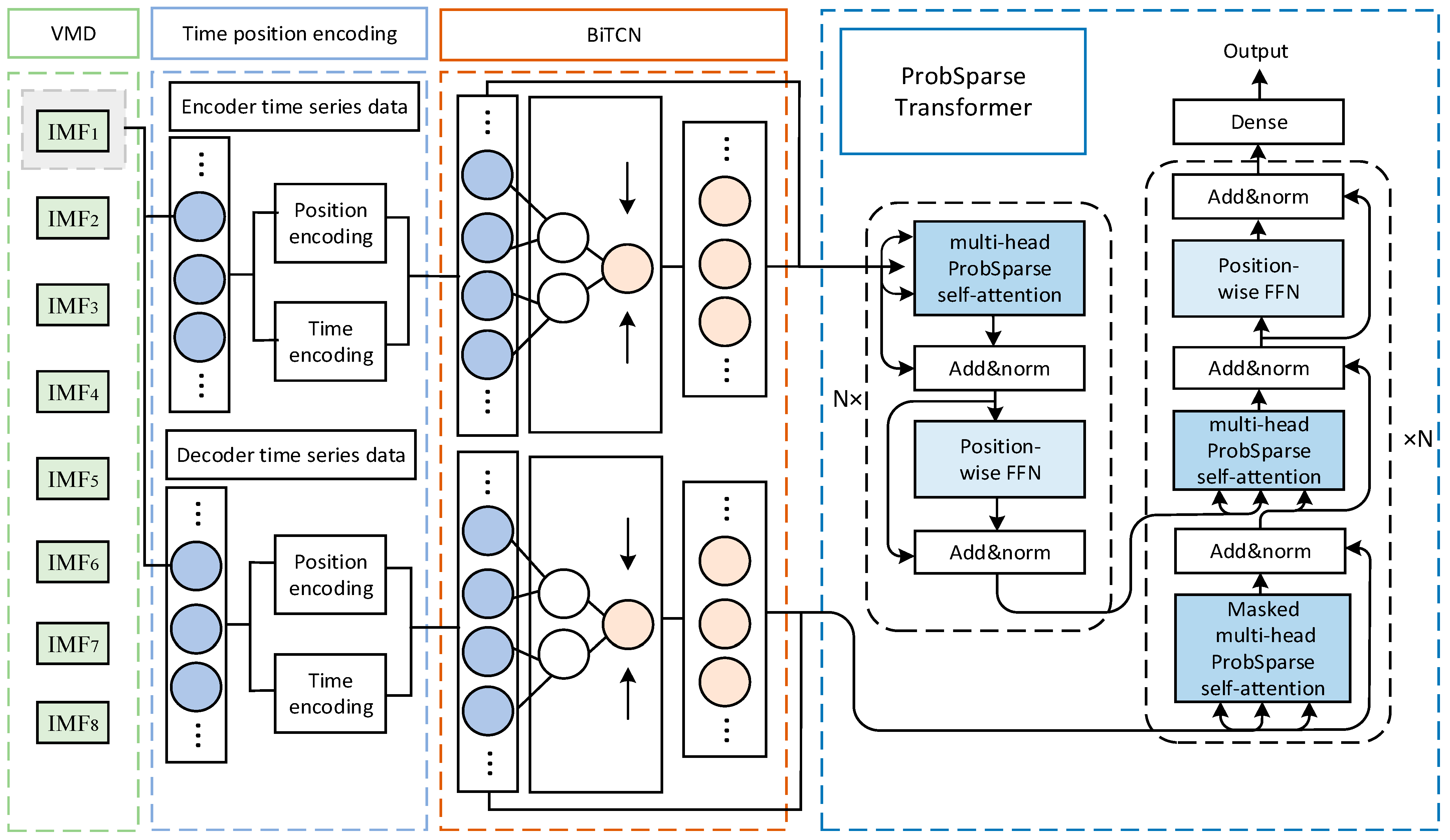
The short-term wind power prediction based on the VMD-BiTCN-Psformer is shown in Figure 6.
Step 1: The VMD technique is employed to decompose the wind power data into several sub-series that exhibit generally stable behavior at different frequencies. This process effectively decreases the complexity and nonlinearity of the sequence.
Step 2: Each sub-mode of the decomposed wind farm original data is mapped to form a time series matrix, and the time features are transformed into dimensions through a one-dimensional convolution layer and then spliced with the improved positional encoding matrix and time series matrix.
Step 3: BiTCN is employed to extract the characteristics of the spliced matrices and capture the enduring connections between them.
Step 4: The output matrix of BiTCN is transformed into query vector and key vector by weight matrix WQ and WK, respectively. The concatenation matrix is transformed into value vector by weight matrix WV. Q, K, V are obtained as matrices by the attention mechanism function, and finally processed to obtain the intermediate feature matrices, which are used in the decoding layer.
Step 5: The output matrix of BiTCN, along with the mask concatenation matrix goes to the decoding layer of Psformer to obtain the query vector. The key vector, the value vector, and the query vector together go to the next sub-layer of the Psformer decoder. The wind power predictions for each sub-mode are derived through the fully connected layer, and then these predictions are aggregated to obtain the final wind power prediction.

4. Results and Discussion

4.1. Data and Evaluation Metrics

The hardware platform used was Intel(R) Core (TM) i7-13, 620H [email protected] GHz and NVIDIA GeForce RTX 4060 Laptop GPU, and CUDA12.3 was used for acceleration. The software platform used was Python3.6 and MATLAB 2022a.
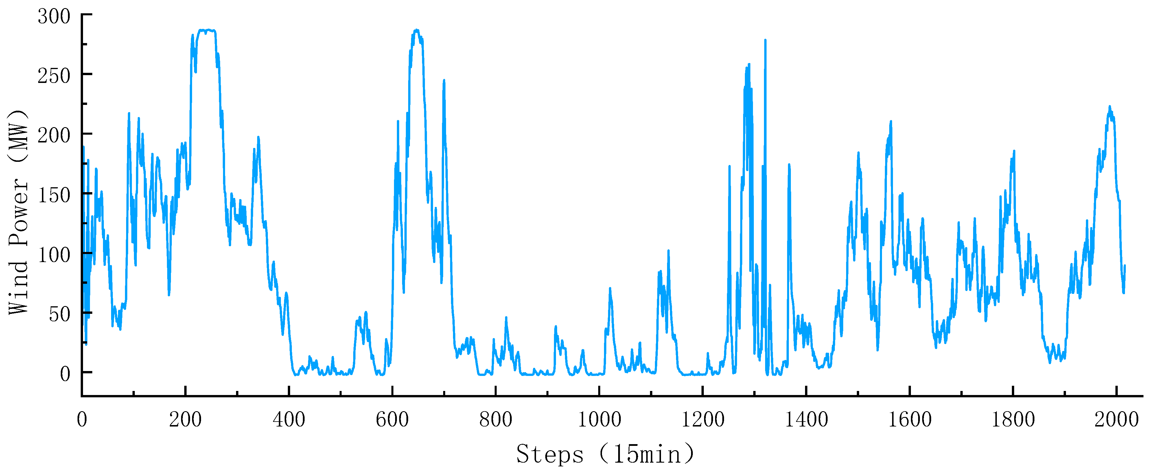
The example data are derived from historical wind power and local meteorological data collected from a wind farm located in Fujian, China. These data includes wind and meteorological data collected from the wind farm between April 6 and April 26, 2023, with measurements taken every 15 min. There are 2016 sets of data in total. The first 20 days’ data are used as the training set to forecast the data for the 21st day. The data contain rich information on variables such as barometric pressure, relative humidity, cloud cover, 10 m wind speed, 100 m wind speed, and temperature. The original wind power data is shown in Figure 7.
Due to the different units of data such as wind turbine output power and wind speed, which are not comparable in their respective dimensions. In order to improve the generalization ability of the model, we trained the hybrid network after normalizing the data sets decomposed by VMD from the original wind power series data; other meteorological data were also normalized into the hybrid model. The normalization is shown in Equation (16).
x = x x min x max x min
where xmin represents the minimum value, xmax represents the maximum value. The data were mapped between [0, 1].
For the normalization of the wind power of the target predicted value, the maximum, and minimum values of the data are saved in an array, which is used for the denormalization of the data after the network forecasting. Finally, the results are restored to the original power interval. The evaluation effect of the model is also based on the results after denormalization. The denormalization is shown in Equation (17).
x = x ( x max x min ) + x min
To reasonably detect the performance of the model, we compared MAE, RMSE, R 2 , and RRMSE using the following equations:
M A E = 1 N i = 1 N x ^ i x i
R M S E = 1 N i = 1 N ( x ^ i x i ) 2
R 2 = 1 i ( x ^ i x i ) 2 i ( x ¯ i x i ) 2
RRMSE = 1 N i = 1 N ( x ^ i x i x i ) 2
where x i represents the actual value, x ^ i represents the predicted value, x ¯ i represents the average value, and N represents the number.
Among them, smaller MAE, RMSE, and RRMSE indicate the better prediction effect, and the closer R 2 to 1, indicates a smaller error.

4.2. Model Parameter Setting

The main parameter settings of the Transformer are shown in Table 1.

4.3. Validation of Model Effectiveness

4.3.1. Comparative Analysis of the Forecasting

To verify the performance of each module, four sets of comparison tests were constructed, as shown in Table 2. “√” indicates that the module was included in the corresponding model. To control the variables, all models used improved positional encoding.
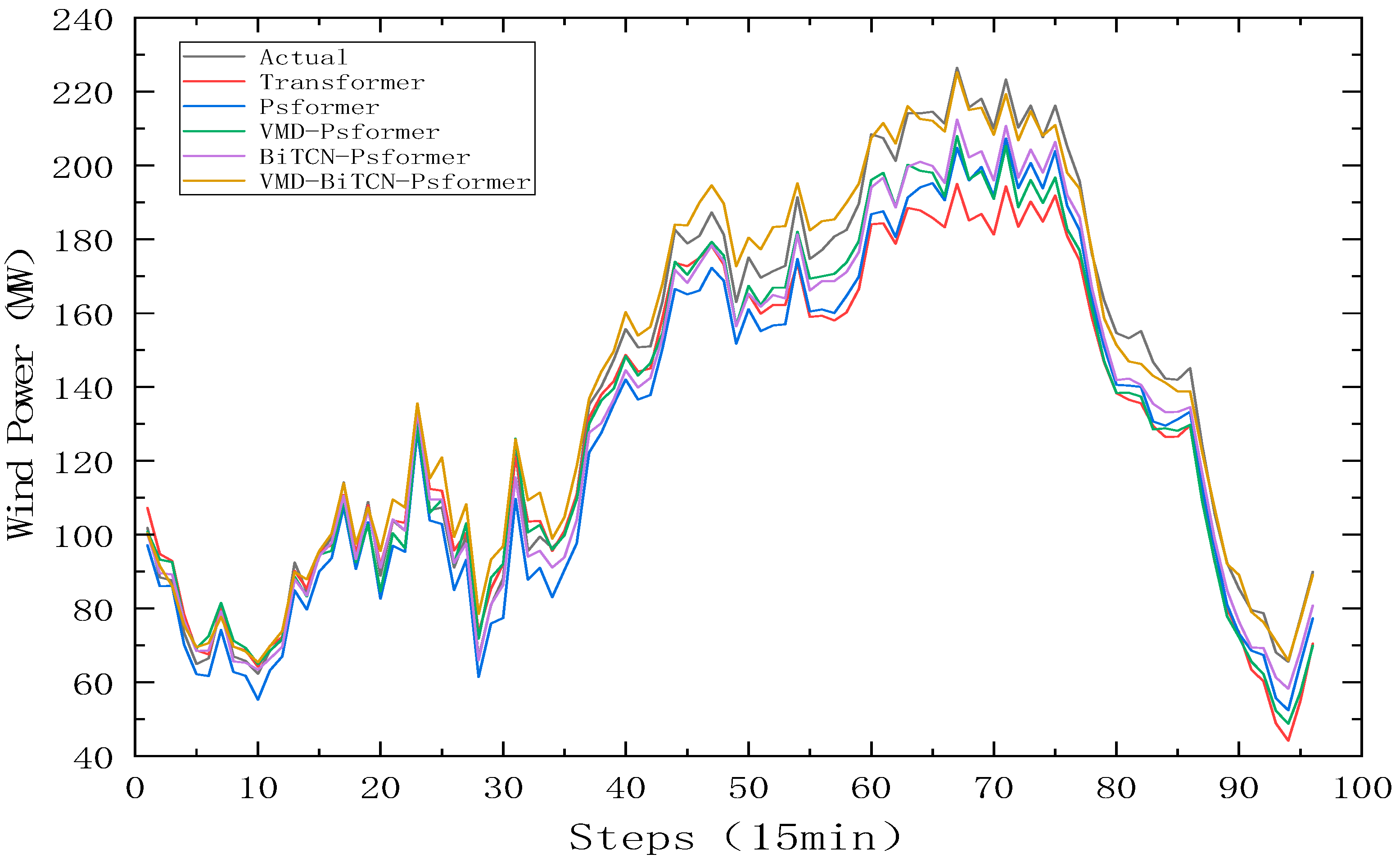
To verify the validity of the module combination, we designed the five models shown in Table 2. Their performance is shown in Table 3. The wind power results are shown in Figure 8. Among all models, the VMD-BiTCN-Psformer model has the best prediction effect.
(1)
Comparing VMD-Psformer with Psformer, and VMD-BITCN-Psformer with BiTCN-Psformer, the MAE of each model decreased by 25.58% and 32.08%, respectively, and the R2 of each model increased by 1.52% and 1.23%, respectively. We found that the prediction effect of the model with VMD is better than that of the model without VMD. The VMD is able to decompose the unstable and highly fluctuating wind power signal into more stable sub-sequences, which greatly improves the accuracy of the model prediction.
(2)
To verify the effectiveness of the improved ProbSparse module, the Psformer model is compared with the Transformer model. We found that Psformer, which discards key values of relatively low importance, performs better in terms of prediction accuracy. The MAE, RMSE, and RRMSE of Psformer are reduced by 1.28%, 18.13%, and 18.12%, respectively, and R2 is increased by 2.73%.
(3)
Compared with Psformer and BiTCN-Psformer, the MAE, RMSE, and RRMSE decreased by 57.92%, 47.60%, and 47.55%, respectively, while R2 increased by 3.64%. BiTCN-Psformer uses BiTCN to adequately capture bi-directional information in time series data, improving the model’s modeling and forecasting performance on sequence data. This means that BiTCN provides a better performance in complex time series tasks.
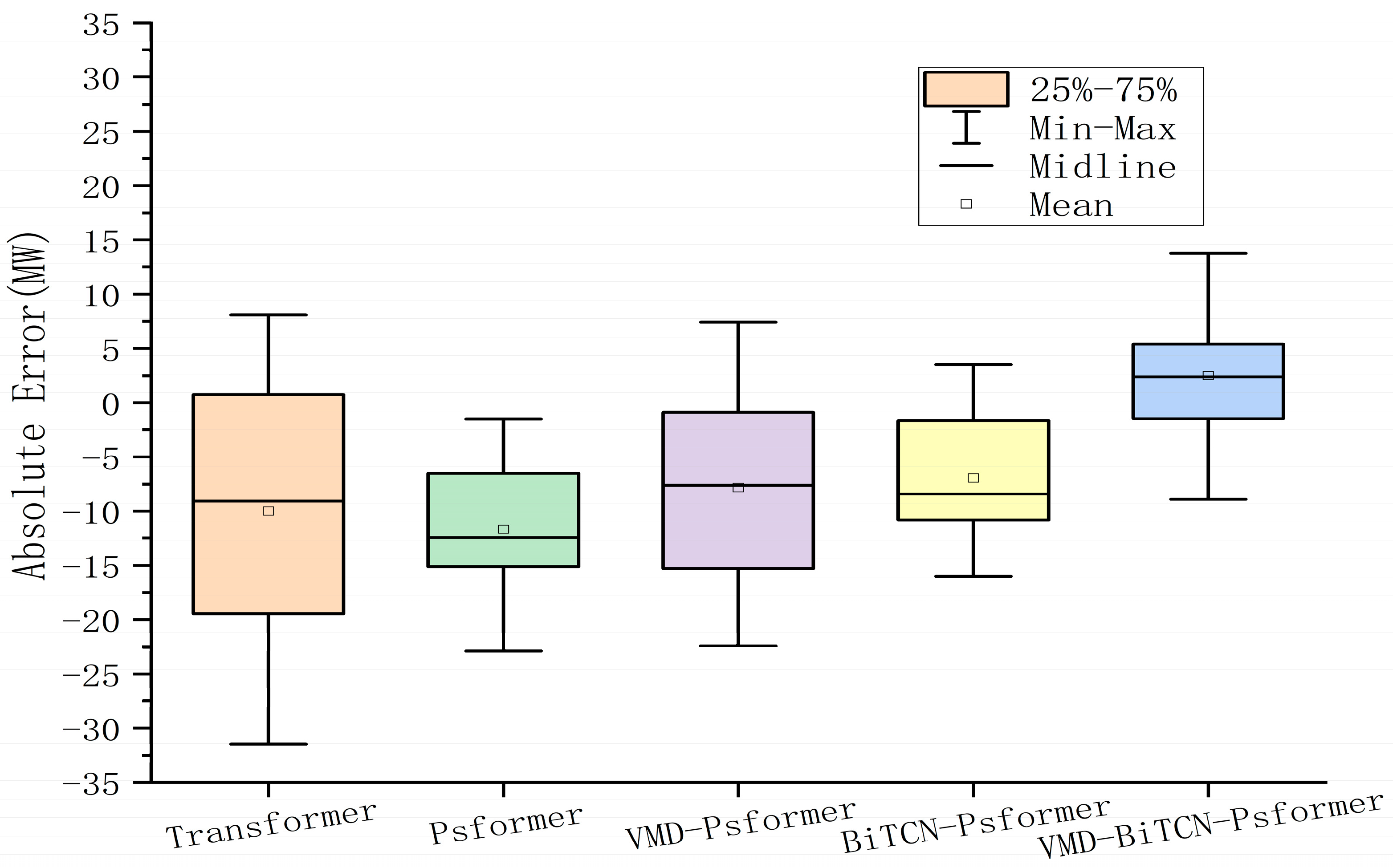
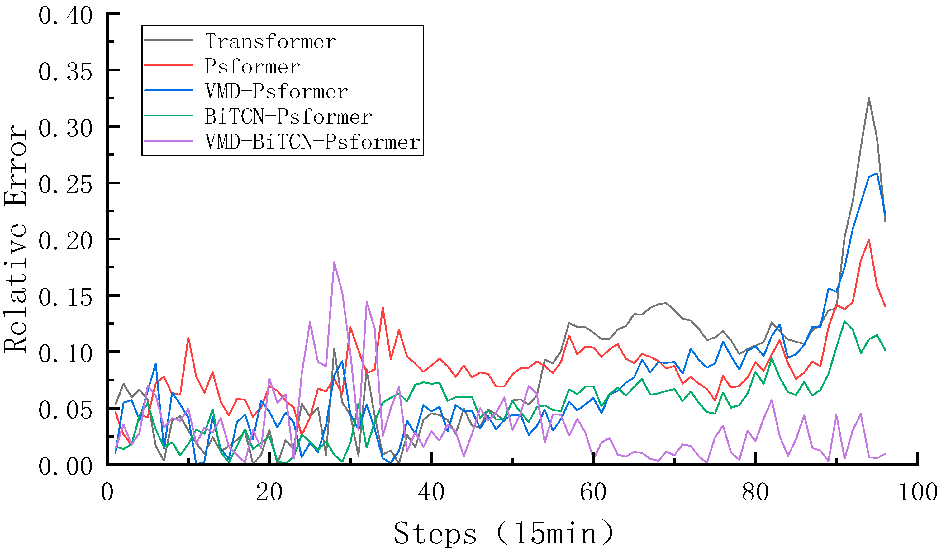
The box plot of the four models’ prediction errors is shown in Figure 9, where it can be seen that the error proposed in this paper is minimized. It can be clearly seen from the relative error shown in Figure 10 that the predicted result of the original transformer has a large deviation from the actual value. The purple part of the figure indicates that the relative error of the model in this paper is at the bottom, and the error is the smallest.

4.3.2. Comparative Analysis with Other Models

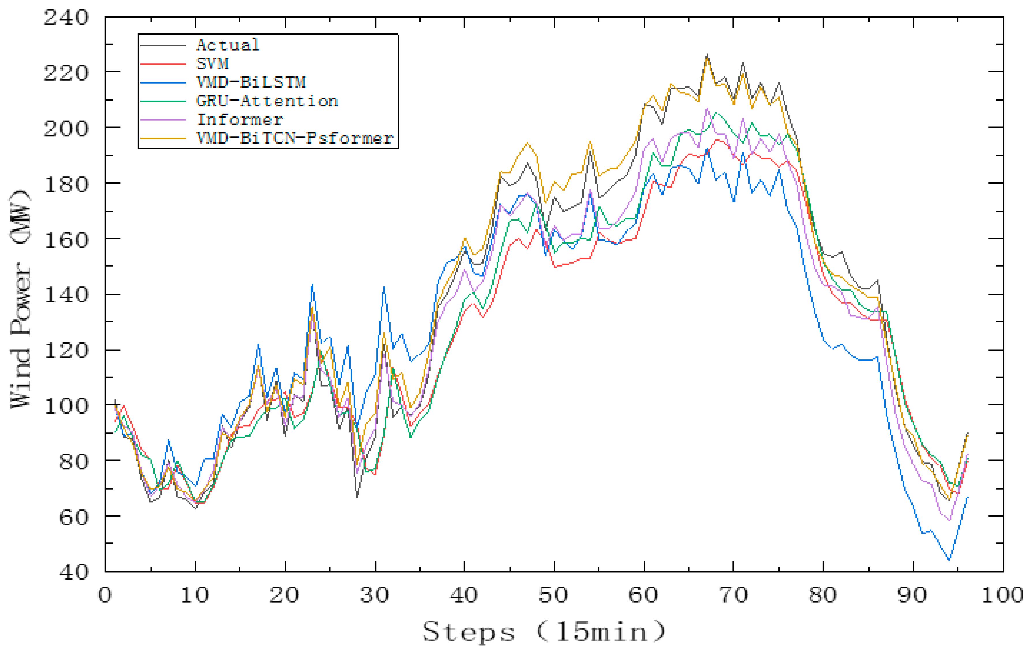
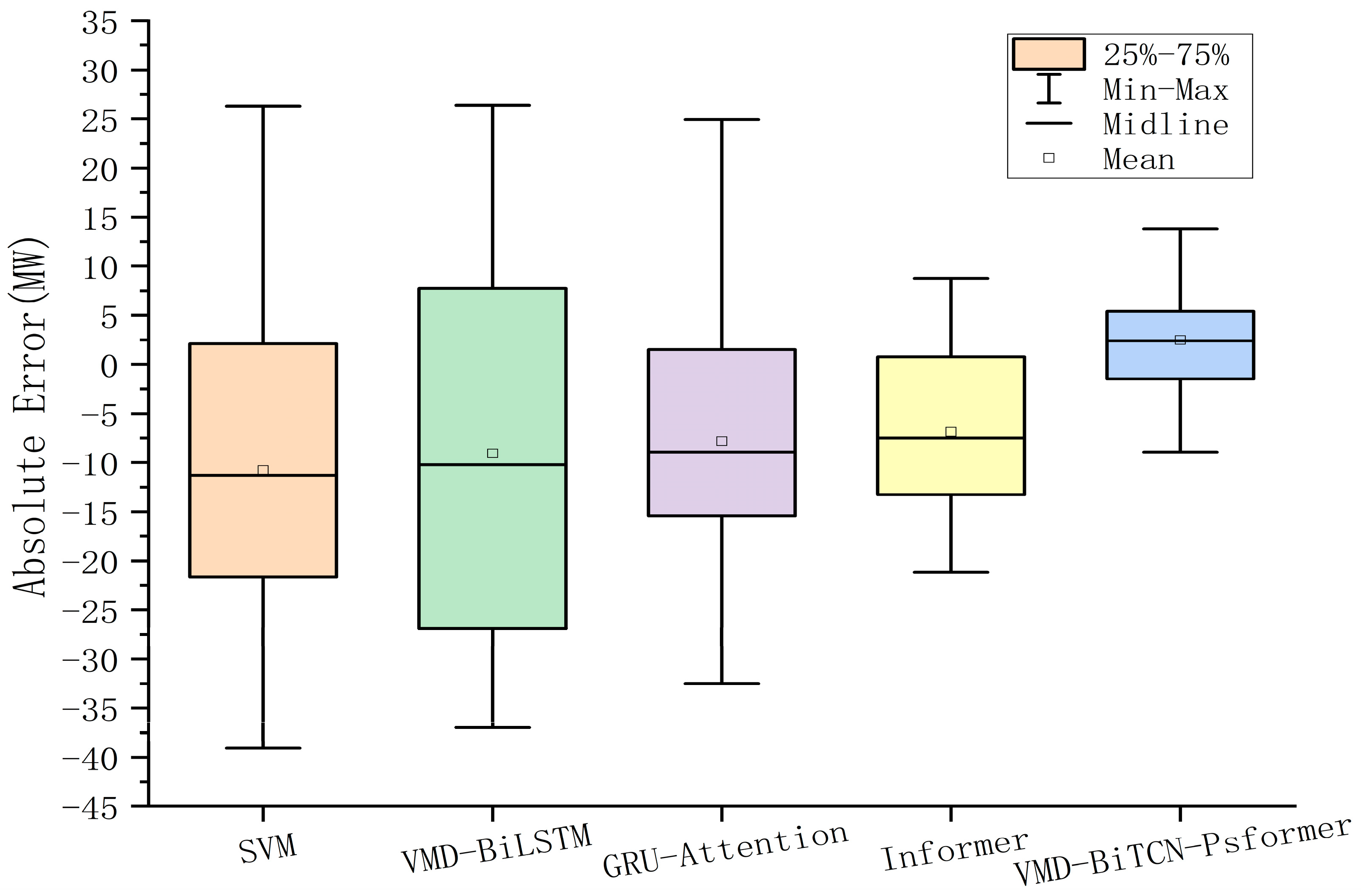
To demonstrate the superior performance of the VMD-BiTCN-Psformer model, we compared it with several other traditional models. We designed four models (SVM, VMD-BiLSTM, GRU-Attention, and Informer) to forecast wind power in a region of Fujian on 26 April 2023. As you can see from Figure 11, the proposed model is closest to the raw power data. The box plot of the different models’ prediction errors is shown in Figure 12. The error values in Figure 12 are larger than the prediction errors in Figure 9.
In Table 4, we compared SVM, VMD-BiLSTM, GRU-Attention, Informer, and VMD-BiTCN-Psformer, in which the error of the VMD-BiTCN-Psformer model is the smallest among all traditional models. Compared with SVM, VMD-BiLSTM, GRU-Attention, and Informer models, the R2 of VMD-BiTCN-Psformer has increased by 22.27%, 12.38%, 8.93%, and 2.59%, respectively. It has been observed that the VMD-BiTCN-Psformer model proposed in this paper possesses the highest accuracy and a better prediction effect.

4.3.3. Forecasting Performance of Improved Positional Encoding

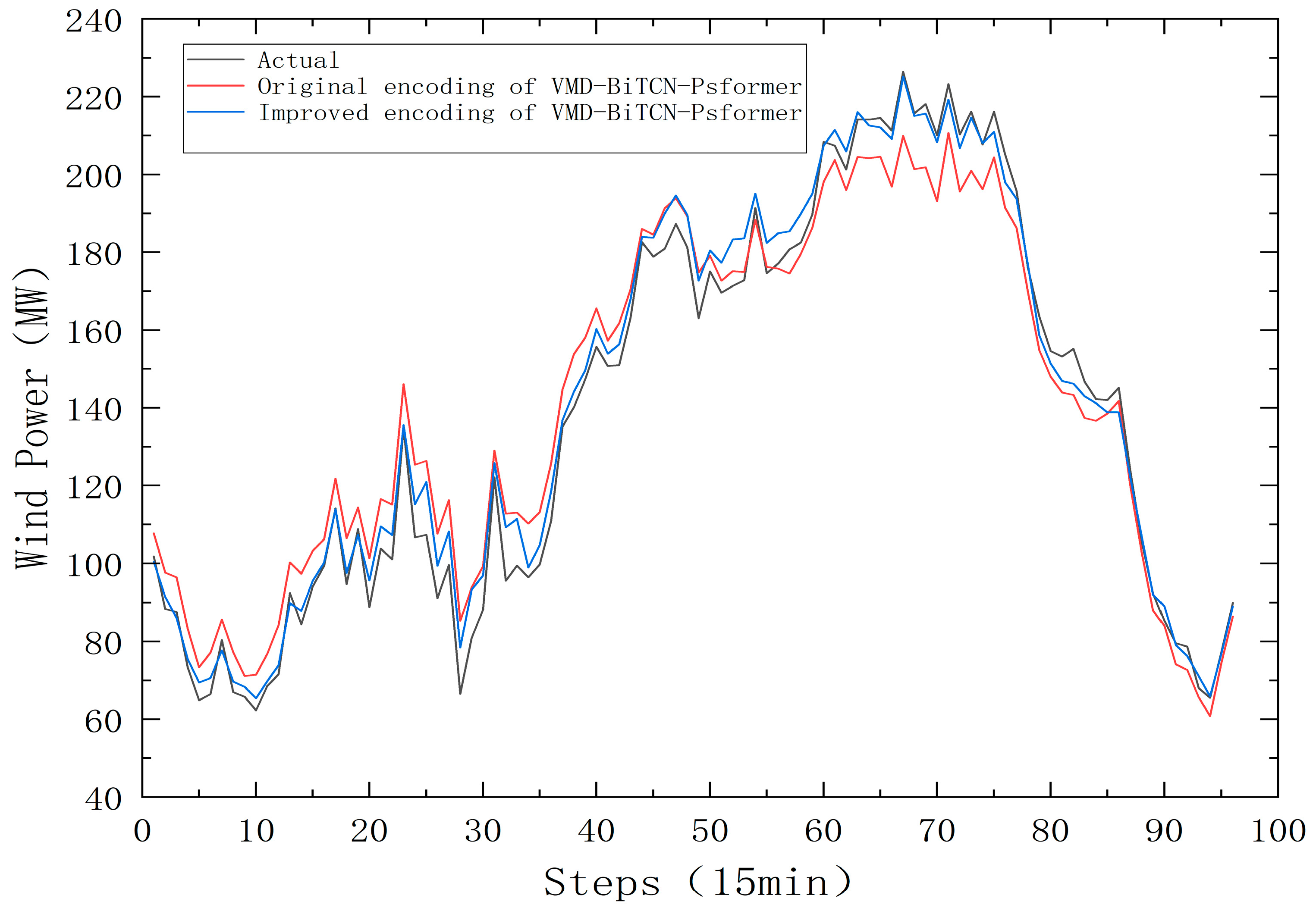
As shown in Figure 13, we also compared the effects before and after the improved position encoding. The data in Table 5 show that the improved positional encoding improves the accuracy of wind power to some extent, and the R2 of the improved position encoding model is higher than that of the original model. The experiments proved that after adding more detailed encoding information, the model was more applicable and the prediction was more accurate.

5. Conclusions

We propose a VMD-BiTCN-Psformer model based on temporal and positional encoding, which aims to improve the accuracy of forecasting wind power.
Combined with the measured wind power data and the meteorological data from a wind farm in Fujian, the proposed VMD-BiTCN-Psformer prediction model was studied:
(1)
The combination model of VMD-BiTCN-Psformer is superior to relatively single combination models, and the application of VMD, BiTCN, and Transformer all contributes to improving the accuracy of predictions.
(2)
Table 4 shows that the MAE, RMSE, RRMSE, and R2 of the wind power prediction results of the proposed model are better than those of other models. The prediction of the designed model is closest to the actual values, so it has a more accurate prediction effect.
(3)
We compared the models before and after improving the positional encoding and found that the prediction accuracy improved after the improvement, demonstrating the effectiveness of the improved encoding.
Our proposed model still has some limitations, which we will continue to study in future work. In the process of VMD, we determined the number of decomposed modes as a fixed value, and it is more effective to optimize VMD parameters by using swarm intelligence algorithm or determine the number of sub-modes according to entropy. At the same time, for power data close to 0, the predicted values of the network model tend to be much higher than the true values, which is an issue that we need to address in our next study.

Author Contributions

Funding acquisition, Q.W.; Methodology, W.X.; Software, W.X.; Supervision, D.L.; Validation, W.X. and Q.W.; Writing—original draft, W.D.; Writing—review and editing, D.L. All authors have read and agreed to the published version of the manuscript.

Funding

This work is supported by the National Natural Science Foundation of China (U1802271).

Data Availability Statement

The original contributions presented in the study are included in the article, further inquiries can be directed to the corresponding author.

Conflicts of Interest

The authors declare no conflicts of interest.

References

  1. Foley, A.M.; Leahy, P.G.; Marvuglia, A.; McKeogh, E.J. Current methods and advances in forecasting of wind power generation. Renew. Energy 2012, 37, 1–8. [Google Scholar] [CrossRef]
  2. Ye, L.; Li, Y.; Pei, M.; Zhao, Y.; Li, Z.; Lu, P. A novel integrated method for short-term wind power forecasting based on fluctuation clustering and history matching. Appl. Energy 2022, 327, 120131. [Google Scholar] [CrossRef]
  3. Liu, H.; Yang, L.; Zhang, B.; Zhang, Z. A two-channel deep network based model for improving ultra-short-term prediction of wind power via utilizing multi-source data. Energy 2023, 283, 128510. [Google Scholar] [CrossRef]
  4. Sun, H.; Cui, Q.; Wen, J.; Kou, L.; Ke, W. Short-term wind power prediction method based on CEEMDAN-GWO-Bi-LSTM. Energy Rep. 2024, 11, 1487–1502. [Google Scholar] [CrossRef]
  5. Zhu, L. Review of Wind Power Prediction Methods Based on Artificial Intelligence Technology. In Proceedings of the 2024 IEEE 7th Advanced Information Technology, Electronic and Automation Control Conference (IAEAC), Chongqing, China, 15–17 March 2024; Volume 7, pp. 1454–1457. [Google Scholar]
  6. Ahmad, T.; Chen, H. A review on machine learning forecasting growth trends and their real-time applications in different energy systems. Sustain. Cities Soc. 2020, 54, 102010. [Google Scholar] [CrossRef]
  7. Shahid, F.; Zameer, A.; Mehmood, A.; Raja, M.A.Z. A novel wavenets long short term memory paradigm for wind power prediction. Appl. Energy 2020, 269, 115098. [Google Scholar] [CrossRef]
  8. Hossain, M.A.; Gray, E.; Lu, J.; Islam, M.R.; Alam, M.S.; Chakrabortty, R.; Pota, H.R. Optimized forecasting model to improve the accuracy of very short-term wind power prediction. IEEE Trans. Ind. Inform. 2023, 19, 10145–10159. [Google Scholar] [CrossRef]
  9. Xiong, B.; Lou, L.; Meng, X.; Wang, X.; Ma, H.; Wang, Z. Short-term wind power forecasting based on Attention Mechanism and Deep Learning. Electr. Power Syst. Res. 2022, 206, 107776. [Google Scholar] [CrossRef]
  10. Niksa-Rynkiewicz, T.; Stomma, P.; Witkowska, A.; Rutkowska, D.; Słowik, A.; Cpałka, K.; Jaworek-Korjakowska, J.; Kolendo, P. An intelligent approach to short-term wind power prediction using deep neural networks. J. Artif. Intell. Soft Comput. Res. 2023, 13, 197–210. [Google Scholar] [CrossRef]
  11. Li, Z.; Ye, L.; Zhao, Y.; Pei, M.; Lu, P.; Li, Y.; Dai, B. A spatiotemporal directed graph convolution network for ultra-short-term wind power prediction. IEEE Trans. Sustain. Energy 2022, 14, 39–54. [Google Scholar] [CrossRef]
  12. Yu, G.Z.; Lu, L.; Tang, B.; Wang, S.Y.; Chung, C.Y. Ultra-short-term wind power subsection forecasting method based on extreme weather. IEEE Trans. Power Syst. 2022, 38, 5045–5056. [Google Scholar] [CrossRef]
  13. Sun, S.; Liu, Y.; Li, Q.; Wang, T.; Chu, F. Short-term multi-step wind power forecasting based on spatio-temporal correlations and transformer neural networks. Energy Convers. Manag. 2023, 283, 116916. [Google Scholar] [CrossRef]
  14. Bentsen, L.Ø.; Warakagoda, N.D.; Stenbro, R.; Engelstad, P. Spatio-temporal wind speed forecasting using graph networks and novel Transformer architectures. Appl. Energy 2023, 333, 120565. [Google Scholar] [CrossRef]
  15. Nascimento, E.G.S.; de Melo, T.A.C.; Moreira, D.M. A transformer-based deep neural network with wavelet transform for forecasting wind speed and wind energy. Energy 2023, 278, 127678. [Google Scholar] [CrossRef]
  16. Xiang, L.; Fu, X.; Yao, Q.; Zhu, G.; Hu, A. A novel model for ultra-short term wind power prediction based on Vision Transformer. Energy 2024, 294, 130854. [Google Scholar] [CrossRef]
  17. Zhou, H.; Zhang, S.; Peng, J.; Zhang, S.; Li, J.; Xiong, H.; Zhang, W. Informer: Beyond Efficient Transformer for Long Sequence Time-Series Forecasting. Proc. AAAI Conf. Artif. Intell. 2020, 35, 11106–11115. [Google Scholar] [CrossRef]
  18. Sheng, Y.; Wang, H.; Yan, J.; Liu, Y.; Han, S. Short-term wind power prediction method based on deep clustering-improved Temporal Convolutional Network. Energy Rep. 2023, 9, 2118–2129. [Google Scholar] [CrossRef]
  19. Chen, Y.; He, Y.; Xiao, J.W.; Wang, Y.W.; Li, Y. Hybrid model based on similar power extraction and improved temporal convolutional network for probabilistic wind power forecasting. Energy 2024, 304, 131966. [Google Scholar] [CrossRef]
  20. Xie, P.; Liu, Y.; Yang, Y.; Lin, X.; Chen, Y.; Hu, X.; Li, L. Offshore wind power output prediction based on convolutional attention mechanism. Energy Sources 2023, 45, 13041–13056. [Google Scholar] [CrossRef]
  21. Kari, T.; Guoliang, S.; Kesong, L.; Xiaojing, M.; Xian, W. Short-Term Wind Power Prediction Based on Combinatorial Neural Networks. Intell. Autom. Soft Comput. 2023, 37, 1437–1452. [Google Scholar] [CrossRef]
  22. Guan, S.; Wang, Y.; Liu, L.; Gao, J.; Xu, Z.; Kan, S. Ultra-short-term wind power prediction method based on FTI-VACA-XGB model. Expert Syst. Appl. 2024, 235, 121185. [Google Scholar] [CrossRef]
  23. Mujeeb, S.; Alghamdi, T.A.; Ullah, S.; Fatima, A.; Javaid, N.; Saba, T. Exploiting deep learning for wind power forecasting based on big data analytics. Appl. Sci. 2019, 9, 4417. [Google Scholar] [CrossRef]
  24. Zhang, D.; Chen, B.; Zhu, H.; Goh, H.H.; Dong, Y.; Wu, T. Short-term wind power prediction based on two-layer decomposition and BiTCN-BiLSTM-attention model. Energy 2023, 285, 128762. [Google Scholar] [CrossRef]
  25. Li, Z.; Luo, X.; Liu, M.; Cao, X.; Du, S.; Sun, H. Wind power prediction based on EEMD-Tent-SSA-LS-SVM. Energy Rep. 2022, 8, 3234–3243. [Google Scholar] [CrossRef]
  26. Yang, M.; Chen, X.; Du, J.; Cui, Y. Ultra-short-term multistep wind power prediction based on improved EMD and reconstruction method using run-length analysis. IEEE Access 2018, 6, 31908–31917. [Google Scholar] [CrossRef]
  27. Liu, H.; Han, H.; Sun, Y.; Shi, G.; Su, M.; Liu, Z.; Wang, H.; Deng, X. Short-term wind power interval prediction method using VMD-RFG and Att-GRU. Energy 2022, 251, 123807. [Google Scholar] [CrossRef]
  28. Xie, T.; Zhang, G.; Liu, H.; Liu, F.; Du, P. A hybrid forecasting method for solar output power based on variational mode decomposition, deep belief networks and auto-regressive moving average. Appl. Sci. 2018, 8, 1901. [Google Scholar] [CrossRef]
  29. Dragomiretskiy, K.; Zosso, D. Variational Mode Decomposition. IEEE Trans. Signal Process. 2013, 62, 531–544. [Google Scholar] [CrossRef]
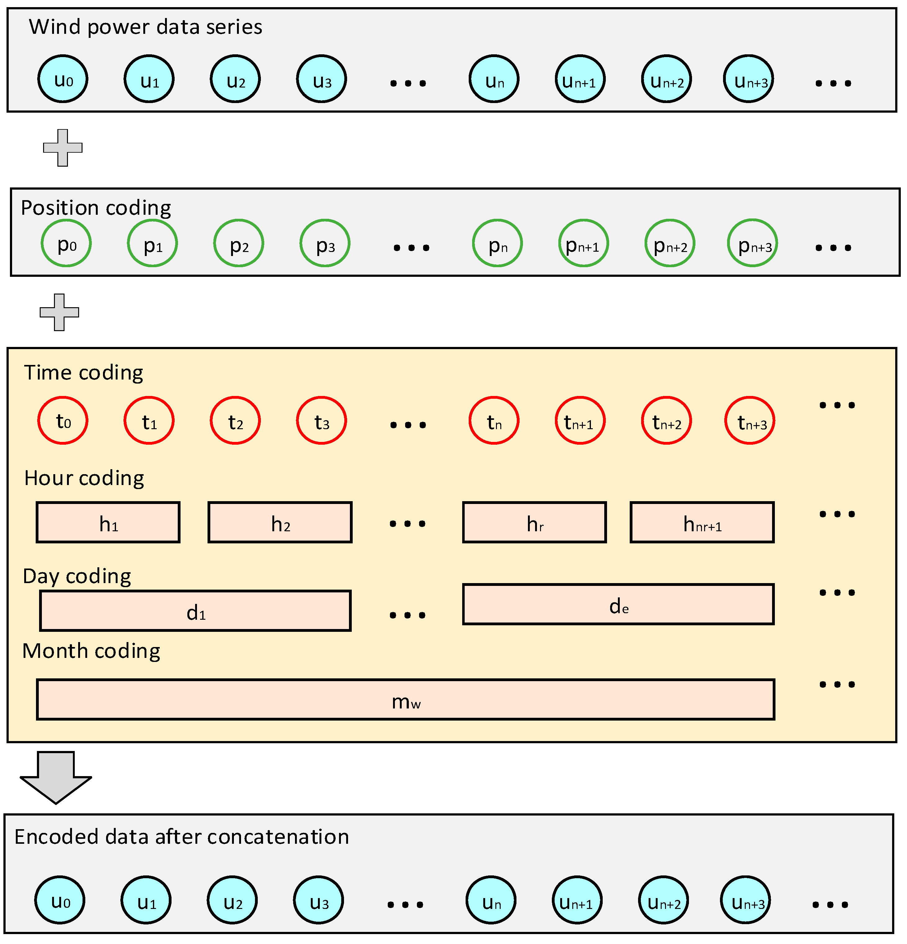
Figure 1. Connection of wind power data, temporal and seasonal information, and positional encoding.
Energies 17 04089 g001
Figure 2. Structure diagram of TCN.
Energies 17 04089 g002
Figure 3. Structure of BiTCN.
Energies 17 04089 g003
Figure 4. The connected structure of multi-head self-attention mechanism after introducing BiTCN.
Energies 17 04089 g004
Figure 5. ProbSparse self-attention mechanism model.
Energies 17 04089 g005
Figure 6. Structure of VMD-BiTCN-Psformer.
Energies 17 04089 g006
Figure 7. Original wind power series data.
Energies 17 04089 g007
Figure 8. Wind power forecast curves of 4 models including Transformer, Psformer, VMD-Psformer, BiTCN-Psformer, and VMD-BiTCN-Psformer.
Energies 17 04089 g008
Figure 9. Box plot of prediction errors for Transformer, Psformer, VMD-Psformer, BiTCN-Psformer, and VMD-BiTCN-Psformer.
Energies 17 04089 g009
Figure 10. The relative error of 4 models including Transformer, Psformer, VMD-Psformer, BiTCN-Psformer, and VMD-BiTCN-Psformer.
Energies 17 04089 g010
Figure 11. Wind power forecast curves of 5 models including SVM, VMD-BiLSTM, GRU-Attention, Informer, and VMD-BiTCN-Psformer.
Energies 17 04089 g011
Figure 12. Box plot of prediction errors for SVM, VMD-BiLSTM, GRU-Attention, Informer, and VMD-BiTCN-Psformer.
Energies 17 04089 g012
Figure 13. Wind power forecast curves of original encoding of VMD-BiTCN-Psformer and improved encoding of VMD-BiTCN-Psformer.
Energies 17 04089 g013
Table 1. Comparison of prediction models.
ParameterSet ValueParameterSet Value
seq_len192batch_size64
enc_in6train_epochs50
dec_in6dropout0.05
sampling factor u5learning_rate0.001
n_head8activationGelu
Table 2. Comparison of different modules.
ModelVMDBiTCNPsformer
Transformer×××
Psformer××
VMD-Psformer×
BiTCN-Psformer×
VMD-BiTCN-Psformer
Table 3. Comparison of module performance of Transformer, Psformer, VMD-Psformer, BiTCN-Psformer, and VMD-BiTCN-Psformer.
ModelEvaluation Metrics
MAERMSE R 2 RRMSE
Transformer11.826215.15590.91200.1030
Psformer11.676212.82980.93690.0872
VMD-Psformer9.298511.30050.95110.0768
BiTCN-Psformer7.39398.69250.97100.0591
VMD-BiTCN-Psformer5.59796.68490.98290.0454
Table 4. Performance comparison of SVM, VMD-BiLSTM, GRU-Attention, Informer, and VMD-BiTCN-Psformer.
ModelEvaluation Metrics
MAERMSE R 2 RRMSE
SVM15.007617.78010.80390.1333
VMD-BiLSTM15.654418.08800.87460.1230
GRU-Attention11.739513.75680.90230.1001
Informer8.642510.45320.95810.0711
VMD-BiTCN-Psformer5.59796.68490.98290.0454
Table 5. Performance of improved positional encoding.
ModelEvaluation Metrics
MAERMSER2RRMSE
Original encoding of VMD-BiTCN-Psformer9.097610.17820.96030.0692
Improved encoding of VMD-BiTCN-Psformer5.59796.68490.98290.0454
Disclaimer/Publisher’s Note: The statements, opinions and data contained in all publications are solely those of the individual author(s) and contributor(s) and not of MDPI and/or the editor(s). MDPI and/or the editor(s) disclaim responsibility for any injury to people or property resulting from any ideas, methods, instructions or products referred to in the content.