Article

Energy Consumption Prediction in Residential Buildings—An Accurate and Interpretable Machine Learning Approach Combining Fuzzy Systems with Evolutionary Optimization

by
Marian B. Gorzałczany
*,† and
Filip Rudziński
Department of Electrical and Computer Engineering, Kielce University of Technology, Al. 1000-lecia P. P. 7, 25-314 Kielce, Poland
*
Author to whom correspondence should be addressed.
These authors contributed equally to this work.
Energies 2024, 17(13), 3242; https://doi.org/10.3390/en17133242
Submission received: 22 May 2024 / Revised: 28 June 2024 / Accepted: 28 June 2024 / Published: 1 July 2024
(This article belongs to the Special Issue Energy Consumption in the EU Countries: 3rd Edition)

Abstract

:
This paper addresses the problem of accurate and interpretable prediction of energy consumption in residential buildings. The solution that we propose in this work employs the knowledge discovery machine learning approach combining fuzzy systems with evolutionary optimization. The contribution of this work is twofold, including both methodology and experimental investigations. As far as methodological contribution is concerned, in this paper, we present an original designing procedure of fuzzy rule-based prediction systems (FRBPSs) for accurate and transparent energy consumption prediction in residential buildings. The proposed FRBPSs are characterized by a genetically optimized accuracy–interpretability trade-off. The trade-off optimization is carried out by means of multi-objective evolutionary optimization algorithms—in particular, by our generalization of the well-known strength Pareto evolutionary algorithm 2 (SPEA2). The proposed FRBPSs’ designing procedure is our original extension and generalization (for regression problems operating on continuous outputs) of an approach to designing fuzzy rule-based classifiers (FRBCs) we developed earlier and published in 2020 in this journal. FRBCs operate on discrete outputs, i.e., class labels. The experimental contribution of this work includes designing the collection of FRBPSs for residential building energy consumption prediction using the data set published in 2024 and available from Kaggle Database Repository. Moreover, the comparison with 20 available alternative approaches is carried out, demonstrating that our approach significantly outperforms alternative methods in terms of interpretability and transparency of the energy consumption predictions made while remaining comparable or slightly superior in terms of the accuracy of those predictions.

1. Introduction

Effective approaches allowing to model the electric energy use and to predict the level of energy consumption in residential buildings are very useful for various reasons related, in general, to building energy performance analysis including, e.g., detecting abnormal energy use patterns [1], determining correct photovoltaics sizing [2], supporting energy management systems [3], modeling predictive control applications using the loads [4], etc.
Significant amounts of data describing various aspects of building energy consumption and their prediction are available now—see, e.g., the most recently published data set [5] that is used in our experiment presented later in this work. It is obvious that a meaningful knowledge on building energy consumption is buried within such data sets. Thus, the development of effective tools for an automatic discovery of such knowledge in the available data sets has a strong rationale; moreover, these data sets constitute a good platform for the application of various machine learning (ML) approaches for performing knowledge discovery tasks. ML was initially defined in 1959 by A. L. Samuel as a “field of study that gives computers the ability to learn without being explicitly programmed” [6]. Presently, ML—partially overlapping the notion of data mining (DM) introduced in the 1990s—also addresses the earlier-mentioned tasks of knowledge discovery in data including an automatic revealing (through learning from data) of valid and understandable decision mechanisms, trends, and patterns hidden in the considered data sets.
Many ML methods have been applied to prediction of energy consumption. A brief review of them is carried out in the next section of this work. Unfortunately, their essential drawback is their non-transparent, non- or hardly interpretable, black-box-type nature that focuses almost exclusively on the accuracy of predictions and does not provide any deeper (or any) explanation, justification, or insight into mechanisms governing predictions they generate. This work is an attempt to address the above-outlined problem by providing an original knowledge-based ML prediction system coming from the field of computational intelligence (CI). CI—a modern extension of traditional artificial intelligence systems—covers “the theory, design, application, and development of biologically and linguistically motivated computational paradigms” [7]. The proposed solution is characterized both by high accuracy and by high interpretability and transparency. To be more specific, it is characterized by genetically optimized accuracy–interpretability trade-off of generated predictions.
As far as the representation of the knowledge learned from data is concerned, among the most transparent and useful structures are conditional IF-THEN-type rules and, in particular, linguistic fuzzy conditional rules [8] due to their high readability, high modularity, and easy-to-grasp interpretation and comprehension by humans. On the other hand, however, methods generating excessive numbers of complex (with many antecedents) rules significantly limit the transparency of the rule-based systems obtained. Therefore, both the accuracy and the interpretability and transparency should be the main performance indices in designing (fuzzy) rule-based systems from data. Considering this, in this paper, we present an original approach to designing fuzzy rule-based prediction systems (FRBPSs). This approach uses separate measures of system accuracy and system interpretability as optimization objectives in the process of building an FRBPS from data. Both optimization objectives have a complementary/contradictory nature. For this reason, a multi-objective evolutionary optimization algorithm (MOEOA) is employed in the process of the FRBPS’s structure and parameter optimization. Such process is equivalent to the FRBPS’s accuracy–interpretability trade-off optimization (see [9] for a review of related work).
The contribution provided by this work is twofold including both methodology and experimental investigations. As far as methodological contribution is concerned, in this paper, we present an original designing procedure of fuzzy rule-based prediction systems (FRBPSs) for accurate and transparent energy consumption prediction in residential buildings. The proposed FRBPSs are characterized by a genetically optimized accuracy–interpretability trade-off. Trade-off optimization is carried out by means of multi-objective evolutionary optimization algorithms. The proposed FRBPSs’ designing procedure is our original extension and generalization (for regression problems) of an approach to designing fuzzy rule-based classifiers (FRBCs) we developed earlier and recently published in this journal [10]. The generalization proposed here in the form of FRBPSs operates on continuous outputs (typical for regression tasks), whereas FRBCs of [10] process only discrete outputs, i.e., class labels (typical for classification tasks). Therefore, from the methodological point of view, the present work can be treated as a continuation and earlier-mentioned generalization of [10], although with different areas of applications ([10] for smart-grid stability prediction and this work for building energy consumption prediction). The experimental contribution of this work includes designing the collection of FRBPSs for residential building energy consumption prediction using the most recently published data set [5]. Moreover, the comparison with as many as 20 available alternative approaches is carried out to demonstrate the advantages and possible drawbacks of the proposed solution.
The remaining part of this work is organized in the following way: First, a review of related work on the application of different ML methods to prediction of energy consumption is presented. Next, the components of the proposed FRBPS design methodology from data through MOEOA-based learning and optimization are briefly presented. In turn, the aforementioned data set used in the reported experiments is characterized. Then, the designing of accurate and interpretable FRBPSs for building energy consumption based on the aforementioned data set as well as a comparative analysis with 20 available alternative methods are carried out and discussed.

2. Related Work

In this paper, we propose an FRBPS (an ML approach) based on multi-objective evolutionary optimization technique and its application to the prediction of energy consumption. For this reason, in this section, we briefly review several alternative ML approaches as well as some multi-objective optimization methods applied to the considered problem. We consider six distinct groups of ML approaches including (1) adaptive neuro-fuzzy inference systems, (2) various types of artificial neural networks, (3) support vector machines/regressions, (4) decision trees and random forests, (5) ensemble approaches, and (6) hybrid approaches. For each of the considered ML types, we briefly review three representative (in our opinion) works; only for a very broad group of artificial neural networks, we review seven works. We also briefly review three representative (in our opinion) papers on the optimization of predictive models for electricity consumption forecasting using multi-objective optimization algorithms. Moreover, we concentrate on the most recently published works, i.e., the works (except for three papers) published since 2021. Reviews of earlier-published papers can be found in [11,12,13].
Adaptive neuro-fuzzy inference systems (ANFISs): As far as ANFISs are concerned, in [14], they are applied to predict electricity consumption of public buildings based on weather conditions and human activities. A set of data samples representing the relationships between weather conditions (seven continuous input attributes), human activities (two categorical input attributes), and electricity consumptions of the library of the Providence University in Taichung, Taiwan (continuous output attribute) and registered between December 2017 and February 2019 (one sample per day) is considered as the benchmark problem. In turn, paper [15] proposes the application of an ANFIS to predict the cooling load in the sector of residential, energy efficiently built buildings. A total of 768 building cases described by eight continuous input attributes (the properties of buildings like overall height, relative compactness, wall area, surface area, roof area, orientation, glazing area, and glazing area distribution) and one output attribute (the cooling load/demand) is considered. In [16], an ANFIS is applied to energy consumption prediction in multi-storey residential buildings. This time, the experimental data set contains measurements of electricity consumed per hour and recorded from January 2010 to December 2010 (8760 measurement samples for 365 days and 24 h per day with four input attributes representing a point in time of measurement: hour of the day, day of the week, day of the month, and month).
Artificial neural networks (ANNs): As already mentioned, various types of ANNs are used in energy consumption prediction tasks. Paper [17] addresses the problem of residential electricity demand drivers in Cameroon using a prediction model based on an ANN. A sample of 1013 questionnaires describing household electricity consumption surveys is used as the empirical context for the application. A single questionnaire contains responses on a total of 40 predictive factors (input attributes) organized into five groups: building factors (number of rooms, rural or urban area, etc.), sociodemographic factors (head of household age, household size, etc.), appliances and lighting factors (number of lamps, the use frequency of fan/air conditioner, etc.), weather factor (average thermal amplitude is only used), and behaviors and attitudes of electricity use (e.g., awareness about energy savings practice). In turn, paper [18] presents an approach to predict electricity consumption for residential buildings where highly irregular human behavior plays a significant role. A Gaussian mixture clustering to detect behavior clusters and an extreme gradient boosting model for classification problems to predict the behavior patterns are combined with an ANN to predict electricity consumption by over 500 residential users placed in a southeastern region of Spain. Input attributes used for prediction cover daily electricity consumption statistics (e.g., mean consumptions during the morning, night, afternoon, and evening), weather statistics (mean, max., and min. temperatures), and calendar data (weekday or holiday and season: summer, winter, or midseason merging autumn and spring). As far as extreme learning machines (ELMs) and wavelet neural networks (WNNs) are concerned, in [19], a multilayer ELM for the prediction of annual building energy consumption is proposed. The approach fuses stacks of autoencoders with an ELM. The data set consists of 5000 residential buildings in the UK described by meteorological metadata and building metadata. In turn, in [20], a type-2 fuzzy WNN is proposed for modeling the energy consumption prediction in residential buildings. The system implementing type-2 fuzzy reasoning using WNN technology is used for the prediction of energy consumption in residential buildings of Northern Cyprus. In [21], a broad survey of many applications of ANNs can be found, including feedforward ANNs (e.g., multilayer perceptrons, radial basis function networks, ELMs, WNNs), recurrent ANNs (e.g., Elman neural networks, long short-term memories, echo state networks, restricted Boltzmann machines), and convolutional ANNs. In turn, paper [22] presents the application of deep neural networks (DNNs) to predict annual building energy consumption with particular emphasis on the effect of building clusters upon the prediction performance. A data set of residential buildings in the UK (5000 cases collected from the Ministry of Housing Communities and Local Government repository) is applied in comparative analysis of DNNs with several alternative ML techniques (see [22] for details). A total of 22 input attributes covering building metadata (e.g., postcodes, floor levels, roof and walls descriptions, number of rooms, window types, etc.), and meteorological data (temperature, wind speed, and pressure taken from Meteostat repository) are considered as predictive factors. In [23], a data collection of 100 buildings described by a total of 20 input attributes including weather conditions (temperature, humidity, wind speed, solar radiation), building properties (number of floors, building area, orientation, window-to-wall ratio, etc.), and environment features (indoor temperature, occupancy, fan and pump efficiency, etc.) is considered as a benchmark problem. An approach based on the rough set theory is used to reduce the dimensionality of data (to select important input attributes), and then an DNN is applied to predict energy consumption in the building. In [11], an overview of selected DNN approaches to forecasting energy consumption in buildings published since 2015 can be found.
Support vector machines/regressions (SVMs/SVRs): As far as SVMs/SVRs are concerned, in [24], the impact of eight input factors (i.e., surface, wall, roof and glazing areas, relative compactness, overall height, orientation, and glazing area distribution) on two output variables (heating and cooling loads) for residential buildings is explored using the SVR-based approach supported by several meta-heuristic optimization algorithms. Paper [25] also applies an SVR combined with some meta-heuristic algorithms to predict heating energy consumption in residential buildings. The prediction is based on the building architectural characteristics and also outdoor temperature (eight input variables are considered). In [26], several prediction modeling approaches (including SVRs) are applied to estimate energy use intensity for US commercial office buildings as well as the individual energy end-uses of HVAC (heating, ventilation, air conditioning) systems, plug loads, and lighting, based upon the Commercial Building Energy Consumption Survey (CBECS) 2012 microdata. The CBECS administered by the US Department of Energy belongs to the most comprehensive publicly available data sets for energy use in commercial buildings in the United States. A sample subset of 1024 office buildings described by 19 continuous and 56 categorical attributes is selected from the original CBECS data and used in the experiments.
Decision trees (DTs) and random forests (RFs): DTs and RFs constitute another class of ML approaches applied to energy consumption prediction problems. In [27], nine ML approaches, including DTs, are compared for energy performance assessment at the stage of residential buildings design. The data set contains 4500 various types of buildings (house, flat, bungalow, and maisonette) collected from the UK Ministry of Housing Communities and Local Government repository. The data set consists of only input attributes (a total of 23 attributes are included) that can be detected and modified at the early design stage (e.g., glazed area, floor description, windows energy efficiency, number of heated rooms) as well as three weather conditions (temperature, wind speed, air pressure). In turn, paper [28] presents the design and implementation of a data-driven building energy benchmarking (BEEM) system for buildings in Singapore. An ensemble tree algorithm for accurately modeling building energy use as well as for identifying the most influential factors is proposed in [28]. The energy disclosure data set (for 1145 buildings) was released by the Building and Construction Authority for the year 2017. A total of 618 buildings with 10 properties as input attributes of the prediction system (e.g., age of building, occupancy, type of air conditioning system, number of rooms) are considered in the experiment. In [29], a particle swarm-optimized RF classification algorithm is proposed to identify the most important factors that contribute to residential heating energy consumption. A data set from smart meters in residential buildings in Tomsk city in Russia is used to test the approach (it contains a total of 18 input attributes covering sensor data, building attribute features like number of floors, wall material, year of construction, etc., as well as weather records).
Ensemble models: An ensemble approach combining long short-term memory and Kalman filter to predict the short-term energy consumption of multi-family residential buildings in South Korea is applied in [30]. The benchmark data set consists of electric consumption measurements for apartments in four residential multi-family (33 floors) buildings and recorded between January and December 2010. Data samples are expressed by 25 input attributes (24 hourly consumption readings and time stamp). In turn, paper [31] performs an overall analysis of energy consumption in smart homes by deploying various ML models including an DT-RF-XGBoost-based ensemble model proposed in [31] (XGBoost denotes eXtreme Gradient Boosting classification algorithm). Two data sets incorporating a total of 503,910 readings from smart meters (with a time span of 1 minute) with 32 features (as input attributes) of house appliances and weather conditions are considered.
Hybrid approaches: Three hybrid approaches are considered in [32], combining an ANN with an evolutionary algorithm (a heap-based optimizer, a multiverse optimizer, and a whale optimization algorithm are considered) to predict building energy consumption in the residential sector. In turn, [33] presents a hybrid approach combining a deep neural network, fuzzy logic, and wavelet transformation yielding the so-called deep neural network-based fuzzy wavelet, supported by particle swarm optimization and a gradient-based learning algorithm, to predict energy consumption in urban buildings of Iranian cities (Tehran, Mashhad, Ahvaz, and Urmia) in the time period from 2010 to 2021. Paper [34] proposes a hybrid neural network prediction model combining convolutional neural networks, a bidirectional gate recurrent unit, an attention mechanism, and residual connection. The energy consumption data of an office building in Guangzhou, China is considered as a case study. The data set includes samples of hourly registered measurements (from 00:00 on 1 September 2020, to 23:00 on 31 August 2021) and described by 10 input attributes (four time factors and two weather, human, and energy factors each).
Multi-objective optimization of electricity consumption predictive models: In [35], the authors indicate that their multi-objective approach can be used to optimize the selection of predictive models by considering objectives such as forecast accuracy, model complexity, and robustness to outliers. However, they do not specify what optimization criteria they use in their experiments. Paper [36] presents an adaptation of a single-objective gray wolf optimization to its bi-objective version (a prediction accuracy and the number of input attributes are considered as two optimization objectives). Finally, in [37], a multi-objective optimization algorithm is used to minimize two objectives, i.e., cooling and heating load prediction errors in buildings.
Concluding, the overwhelming majority of the above-reviewed studies presents the exclusively prediction accuracy-oriented techniques, i.e., black-box, non-transparent systems not providing any insight into the internal mechanisms governing the prediction of energy consumption. It is worth emphasizing that interpretability and transparency are included in the list of future directions of research on energy consumption prediction. For instance, according to the most recently published work [38], “Future research in energy forecasting should aim to enhance data preprocessing methods, develop more interpretable and less computationally demanding models, and increase the adaptability of forecasting techniques” (a quote from [38]). Our paper is an attempt to address that problem and to fill that knowledge gap.

3. Methodology: Designing Fuzzy Rule-Based Prediction Systems (FRBPSs) from Data Using Multi-Objective Evolutionary Optimization Algorithms (MOEOAs)

The proposed approach employs MOEOAs to develop design from data FRBPSs that are characterized by genetically optimized accuracy–interpretability trade-off. Such FRBPSs can provide both accurate and interpretable predictions in a given domain—in particular, in the building energy consumption domain. As we already mentioned in the Introduction of this work, the proposed FRBPS design procedure is our original generalization (for regression problems usually operating on continuous outputs) of the earlier-developed by us and recently published in this journal [10] fuzzy classifier (operating on discrete outputs, i.e., class labels typical in classification tasks). Therefore, in this section, we particularly concentrate on all newly introduced elements of the FRBPS designing procedure, briefly addressing the remaining ones. First, the FRBPS structure, attribute representation, knowledge base, and fuzzy approximate inference engine are presented. Then, FRBPS genetic learning and MOEOA-based optimization are outlined including the learning data set, objectives of the FRBPS’s evolutionary optimization, and the MOEOA used.
FRBPS’s structure and attribute representation: Consider a system (an FRBPS) with n input attributes x 1 , x 2 , , x n ( x i X i , i = 1 , 2 , , n ), including both numerical and categorical (qualitative) attributes. and an output attribute y ( y Y ).
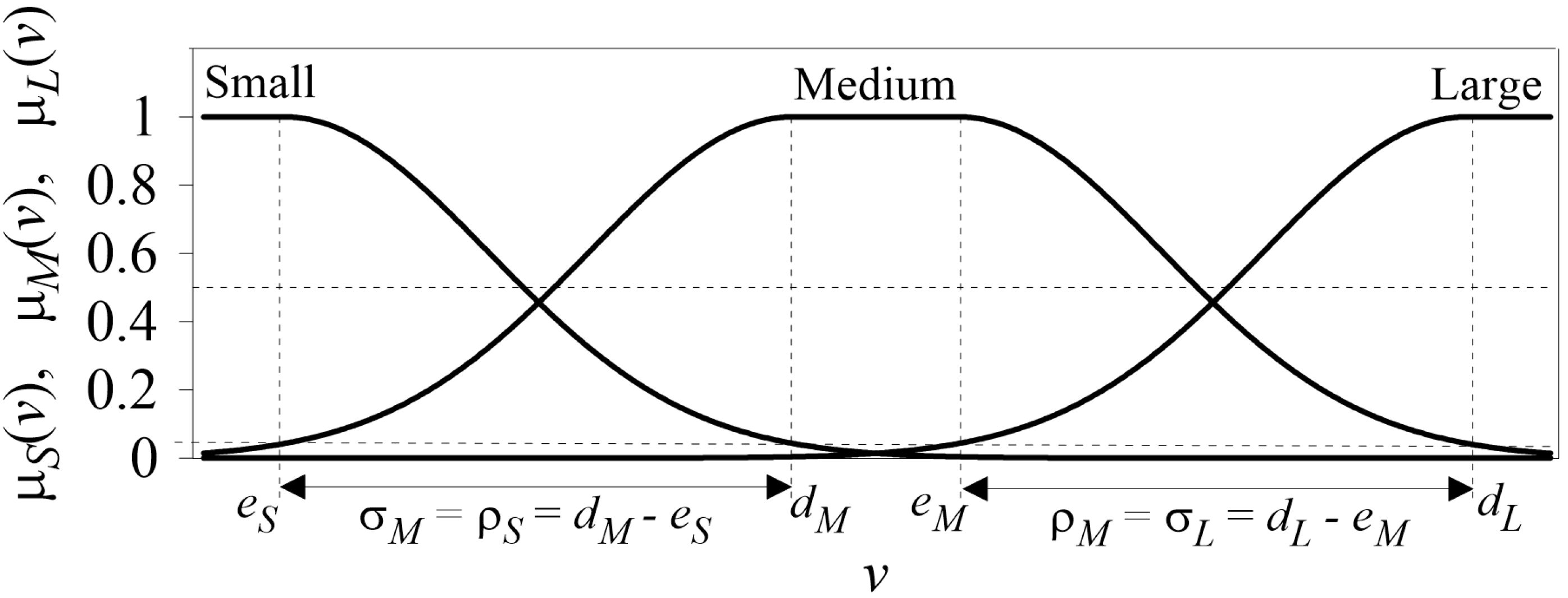
We let F ( X i ) , i = 1 , 2 , , n and F ( Y ) denote families of all fuzzy sets defined in universes X i , i = 1 , 2 , , n , and Y, respectively. As far as numerical input attributes are concerned, each attribute x i X i , i { 1 , 2 , , n } (see such attributes in Table 1 later in the paper) is characterized by a i fuzzy sets A i k i F ( X i ) , k i = 1 , 2 , , a i . A i 1 denotes an S-type fuzzy set (representing linguistic term “Small”), A i a i denotes an L-type set (representing linguistic term “Large”), and A i 2 , A i 3 , , A i , a i 1 denote M-type sets (representing linguistic terms “Medium 1”, “Medium 2”, …, “Medium a i 2 ”). Similarly, a numerical output attribute (see such an attribute also in Table 1) is characterized by b fuzzy sets B k o u t F ( Y ) , k o u t = 1 , 2 , , b . B 1 denotes an S-type fuzzy set, B b —an L-type fuzzy set, and B 2 , B 3 , , B b 1 M-type fuzzy sets (particular fuzzy sets represent appropriate linguistic terms as in the case of input attributes). For simplicity, A i k i s and B k o u t s also denote the corresponding linguistic terms. Membership functions of S-, M-, and L-type fuzzy sets used in our experiments are of the following form (variable v stands for any input attribute x i , i = 1 , 2 , , n and output attribute y; see Figure 1):
μ S ( v ) = 1 , for   v e S , f G ( v e S ρ S ) , for   v > e S ,
μ M ( v ) = f G ( v d M σ M ) , for   v d M , 1 , for   d M < v e M , f G ( v e M ρ M ) , for   v > e M ,
μ L ( v ) = f G ( v d L σ L ) for   v d L , 1 , for   v > d L ,
where e S < d M e M < d L , ρ S > 0 , σ M > 0 , ρ M > 0 , σ L > 0 , and f G ( τ ) is a Gaussian-type function, i.e.,
f G ( τ ) = e τ 2 .
As mentioned earlier in this section, one S-type, one L-type, and usually several M-type fuzzy sets can be considered for a given attribute. We emphasize that a given linguistic term for a given input/output attribute is represented by the same fuzzy set in all fuzzy rules in which it occurs.
As far as categorical input attributes are concerned (see attributes of that type in Table 1 later in the paper), each attribute x i X i = { x i 1 , x i 2 , , x i a i } , i { 1 , 2 , , n } is characterized by a i fuzzy singletons A i k i = A i k i ( s i n g l . ) F ( X i ) , k i = 1 , 2 , , a i defined for particular “values” x i k i of x i as follows: μ A i k i ( s i n g l . ) ( x i ) = 1 for x i = x i k i , and 0 elsewhere.
FRBPS knowledge base: It contains R genetically optimized fuzzy IF-THEN rules discovered during the evolutionary learning and optimization process presented later in this section. We propose the following form of the rth rule, r = 1 , 2 , , R (the number of rules R changes during the learning process):
IF [ x 1   i s   [ n o t ]   ( s w 1 ( r ) < 0 )   A 1 , | s w 1 ( r ) | ] ( s w 1 ( r ) 0 ) AND [ x i   i s   [ not ]   ( s w i ( r ) < 0 )   A i , | s w i ( r ) | ] ( s w i ( r ) 0 ) AND [ x n   is   [ not ]   ( s w n ( r ) < 0 )   A n , | s w n ( r ) | ] ( s w n ( r ) 0 ) THEN   y   is   B k o u t ( r ) ,
where
(i)
[ e x p r e s s i o n ] ( c o n d i t i o n ) in (5) represents conditional inclusion of [ e x p r e s s i o n ] into a considered rule if and only if ( c o n d i t i o n ) is fulfilled,
(ii)
| · | return the absolute value,
(iii)
s w i ( r ) , i = 1 , 2 , , n , r = 1 , 2 , , R are switch-parameters (set and modified by an MOEOA) that control the presence/absence of the ith input attribute in the rth fuzzy rule. s w i ( r ) { 0 , ± 1 , ± 2 , , ± a i } , where a i is the earlier-defined number of fuzzy sets (and the corresponding linguistic terms) that represent the ith input attribute. s w i ( r ) are defined as follows:
-
for s w i ( r ) = 0 , the ith input attribute is excluded from (not active in) the rth rule,
-
for s w i ( r ) > 0 , the component [ x i   is   A i k i ] ( k i = s w i ( r ) ) is included in the rth rule,
-
for s w i ( r ) < 0 , the component [ x i   is   not   A i k i ] ( k i = | s w i ( r ) | ) is included in the rth rule (not A i k i = A ¯ i k i and μ A ¯ i k i ( x i ) = 1 μ A i k i ( x i ) ; μ A i k i ( x i ) and μ A ¯ i k i ( x i ) are membership functions of fuzzy sets A i k i and A ¯ i k i , respectively).
The FRBPS knowledge base is implemented using two separate modules, i.e., a rule-base-structure module R B S and a rule-base-data module R B D . We introduce a simple, direct, and thus computationally efficient R B S representation in the following form:
R B S = { s w 1 ( r ) , s w 2 ( r ) , , s w n ( r ) , k o u t ( r ) } r = 1 R .
In turn, the R B D module contains tunable and non-tunable parts. The tunable part contains parameters of membership functions of fuzzy sets representing linguistic terms for particular numerical input and output attributes. These parameters are subject to tuning during FRBPS learning and MOEOA-based optimization. The considered parameters include (see Figure 1) e S and ρ S for S-type fuzzy sets, σ M , d M , e M , and ρ M for M-type fuzzy sets as well as σ L and d L for L-type fuzzy sets. The non-tunable part of R B D contains domains of categorical input attributes X i = { x i 1 , x i 2 , , x i a i } , i { 1 , 2 , , n } .
We develop original crossover and mutation operators for the processing of the population of R B S s as well as some specialized crossover and mutation operators for the transformation of the population of R B D s; see, for details, the earlier-mentioned work [10] we recently published in this journal.
FRBPS’s approximate inference engine: During the genetic learning process, an evaluation of particular individuals (fuzzy rule bases) competing with each other in the framework of Pittsburgh-type genetic approach used, cf. [39,40], must be performed in each generation. For this reason, a fuzzy set theory-based representation of linguistic IF–THEN rules (5) must be defined and a fuzzy approximate inference engine must be employed. Various definitions of fuzzy implications (see, e.g., [41]) can be implemented in our approach. The most often applied is the so-called Mamdani’s model (see, e.g., [42] for details), which uses min-operation for combining many rule antecedents (input attributes) and rule antecedents with rule consequents (input and output attributes) as well as max-operation for rule aggregation. Employing the aforementioned most often used Mamdani’s approach, we obtain, for input numerical data x = ( x 1 , x 2 , , x n ) , an FRBPS fuzzy-set response B F ( Y ) characterized by its membership function μ B ( y ) , y Y :
μ B ( y ) = max r = 1 , 2 , , R μ B ( r ) ( y ) = max r = 1 , 2 , , R min [ α ( r ) , μ B k o u t ( r ) ( y ) ] ,
where
α ( r ) = min i = 1 , 2 , , n , s w i ( r ) 0 α i ( r ) ,
and
α i ( r ) = μ A i , s w i ( r ) ( x i ) , for   s w i ( r ) > 0 , μ A ¯ i , | s w i ( r ) | ( x i ) , for   s w i ( r ) < 0 .
α ( r ) is the activation degree of the rth fuzzy rule by input numerical data x , whereas α i ( r ) for i such that s w i ( r ) 0 is the activation degree of the ith input attribute in that rule.
If an FRBPS’s non-fuzzy response y is required, it is calculated using a “half of the field” approach as follows:
y = arg min y 0 Z | ʃ y 0 μ B ( y ) ʃ y 0 μ B ( y ) | .
FRBPS’s learning data set: The proposed prediction system is designed during the genetic learning and MOEOA-based optimization process from learning data set L that contains K input–output samples:
L = { x k ( l r n ) , y k ( l r n ) } k = 1 K ,
where x k ( l r n ) = ( x 1 k ( l r n ) , x 2 k ( l r n ) , , x n k ( l r n ) ) X = X 1 × X 2 × × X n (× stands for Cartesian product of ordinary sets) is the collection of input attributes and y k ( l r n ) is the corresponding output attribute ( y k ( l r n ) Y ) for the kth data sample, k = 1 , 2 , , K .
FRBPS’s evolutionary optimization objectives: Two separate optimization objectives are employed, i.e., the accuracy and the interpretability of the system. The FRBPS accuracy measure (subject to maximization) is defined in the following way:
Q A C C ( l r n ) = 1 1 y max y min Q R M S E ( l r n ) ,
where
Q R M S E ( l r n ) = 1 K k = 1 K ( y k ( l r n ) y k ) 2 .
Q A C C ( l r n ) [ 0 , 1 ] , [ y min , y max ] is the range of values of y k ( l r n ) , y k is the system’s non-fuzzy response (10) to the kth learning data sample x k ( l r n ) , and y k ( l r n ) is the desired response for that sample; see (11); Q R M S E ( l r n ) is the root mean square error of our approach in the learning data set.
The FRBPS interpretability embraces two aspects: a complexity-related interpretability and a semantics-related interpretability. As far as the FRBPS’s complexity-related interpretability is concerned, its measure (subject to maximization) is defined as follows:
Q I N T = 1 Q C P L X ,
where
Q C P L X = Q R I N P + Q I N P + Q F S 3 ,
and
Q R I N P = 1 R r = 1 R n I N P ( r ) 1 n 1 ,   Q I N P = n I N P 1 n 1 ,   Q F S = n F S 1 i = 1 n a i 1 ,   n > 1 .
The FRBPS complexity measure Q C P L X (15) ( Q C P L X [ 0 , 1 ] ; 0 and 1 represent minimal and maximal complexities, respectively) is an average of three sub-measures that evaluate
(i)
an average complexity of particular rules Q R I N P (16) ( n I N P ( r ) in (16) is the number of active input attributes in the rth rule),
(ii)
the complexity of the whole system related to the number of its active inputs Q I N P (16) ( n I N P in (16) denotes the number of active inputs in the whole system), and
(iii)
the complexity of the whole system related to the number of its active fuzzy sets Q F S (16) ( n F S in (16) is the number of active fuzzy sets (linguistic terms) in the whole system).
The FRBPS semantics-related interpretability is implemented by imposing, as optimization constraints, the so-called strong fuzzy partitions (SFPs) [43] upon domains of all numerical input and output attributes. SFPs are fuzzy partitions in which the sum of the values of membership functions of all fuzzy sets (fuzzy partitions) for any domain value are roughly equal to 1; it means that neighboring fuzzy sets overlap each other on a roughly 0.5-level, which means a good coverage of the considered domain. Straightforward implementation of SFP requirements for the case of Gaussian-like membership functions can be formulated in the following way (see Figure 2 for illustration of the implementation of the SFP-requirements for the three-set SFP of the v domain):
σ i k i = ρ i , k i 1 = d i k i e i , k i 1 , k i = 2 , 3 , , a i
and
e i 1 < d i 2 e i 2 < d i , a i 1 e i , a i 1 < d i a i ,   i = 1 , 2 , , n .
The FRBPS accuracy and interpretability measures used as evolutionary optimization objectives guide the optimization process carried out by an appropriate MOEOA. In our experiments reported in this work, we use our generalization of one of the well-known MOEOAs, i.e., the strength Pareto evolutionary algorithm 2 (SPEA2) [44]. That generalization, referred to as SPEA3, is introduced in [45] and briefly presented in the earlier-mentioned paper [10] published recently in this journal (see also [46]). The essence of our generalization of SPEA2 consists in changing the original mechanism responsible for the selection of non-dominated solutions during the optimization process. In our SPEA3, this mechanism is replaced by our original environmental selection procedure, which aims at maintaining the best possible spread (i.e., the longest possible distance between extreme solutions in the objective space), the best possible balance (i.e., keeping possibly equal distances between adjacent solutions in the objective space), and the high diversity of solutions occurring in Pareto-front approximation. As a result of that, the proposed SPEA3 is characterized by better performance than SPEA2. SPEA3 generates sets of solutions that are more accurate and characterized by higher spread and better balanced distribution in the objective space than alternative solutions generated by SPEA2. The details concerning the operation of our SPEA3 can be found in [45].

4. Energy Consumption Prediction Data Set Considered

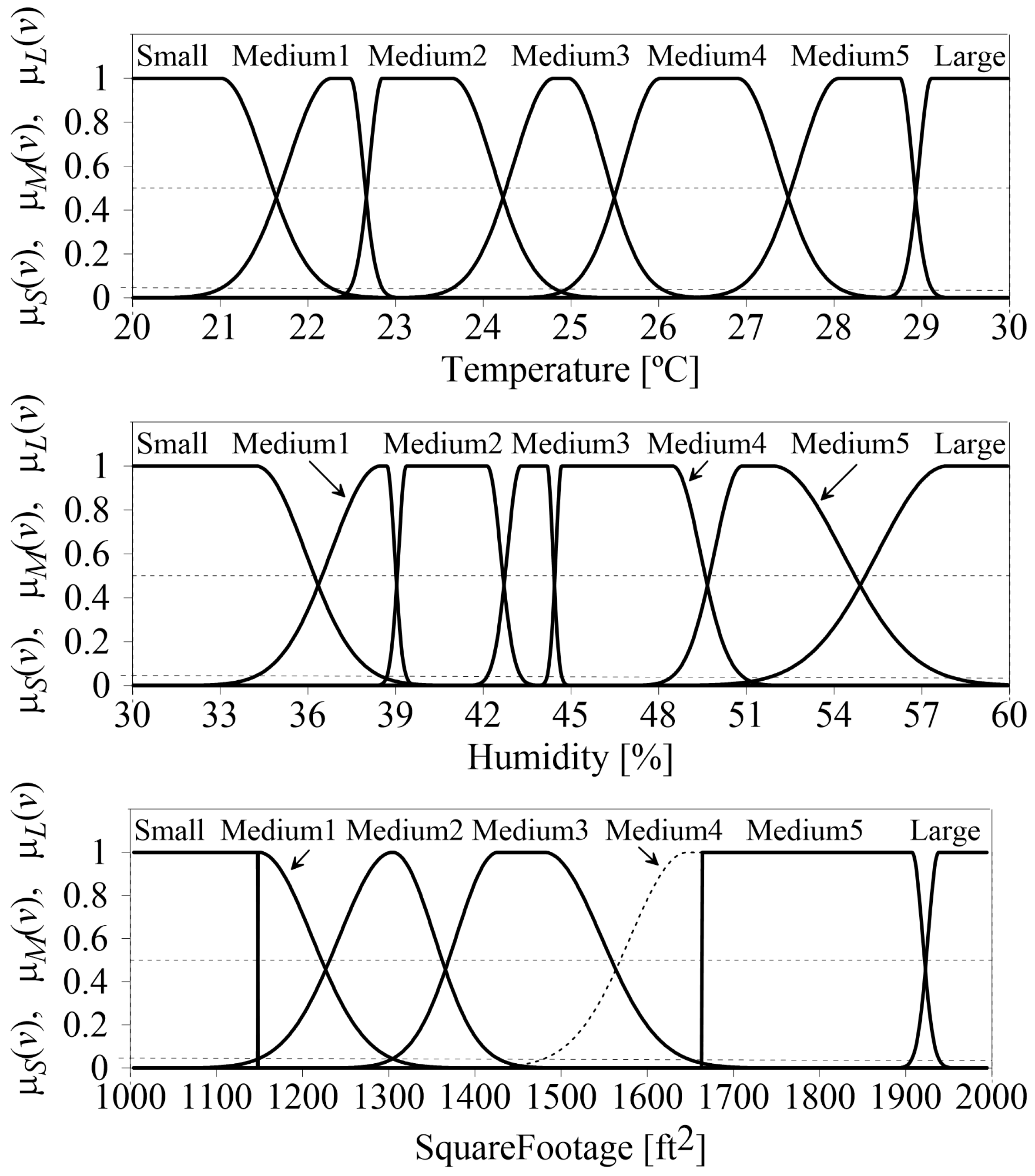
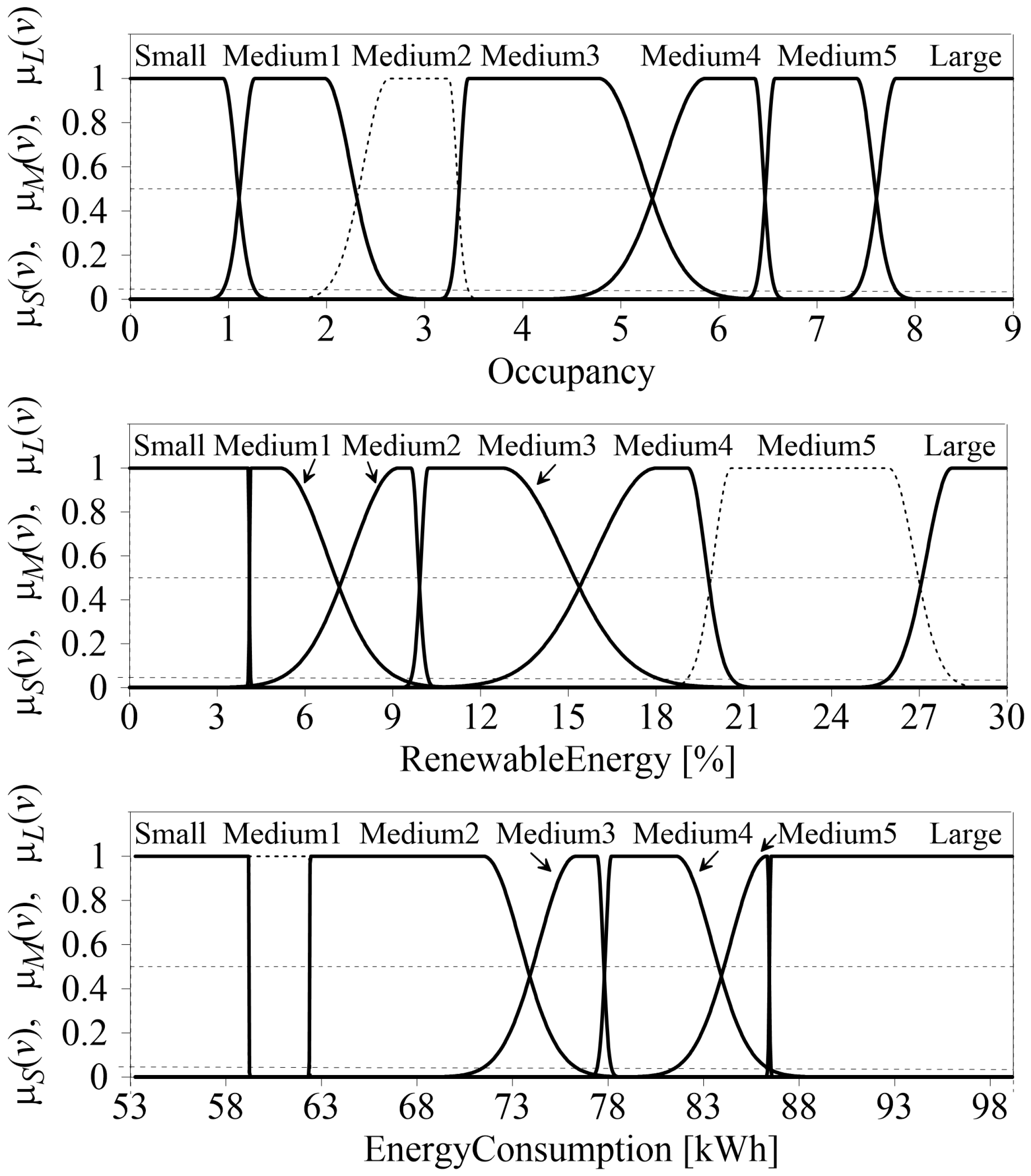
As already mentioned in the introductory section of this paper, the most recently published data set, available (on 15 April 2024) from https://www.kaggle.com/datasets/mrsimple07/energy-consumption-prediction/data [5] and describing various aspects of building energy consumption and its prediction, is considered in our experiments. It is designed to emulate real-world scenarios related to energy usage encapsulating the influence of a diversified list of attributes including temperature, humidity, HVAC (heating, ventilation, air conditioning), and lighting usage, renewable energy contribution, occupancy, square footage, etc., of residential buildings upon energy consumption (see [5] for comments). The considered data set contains 1.000 records (instances) without missing values. Each record is characterized by 10 input attributes and 1 output (target) attribute. Input attributes include five numerical ones (four real and one integer), four categorical (qualitative) ones and the timestamp; the output attribute (to be predicted), i.e., the energy-consumption level, is numerical (real) one; see Table 1 for details. According to some psychological findings (see [43] and particularly [47]), “the number of conditions in the antecedent of a rule must not exceed the limit of 7 ± 2 distinct conditions, which is the number of conceptual entities a human being can handle” (quotation from [43]). Extending that principle for the number of linguistic terms (fuzzy sets) for numerical attributes as well as having in mind a satisfactory performance of the prediction system obtained, we use seven linguistic terms (fuzzy sets) for each numerical attribute; initial shapes of membership functions of those fuzzy sets are shown in Figure 3. A bigger number of fuzzy sets out of which our approach selects the most appropriate ones for a given fuzzy rule (see the next section) improves the overall performance of the prediction system (the rule precision, accuracy, and transparency).

5. Experiments (Application of Our Approach to Prediction of Building Energy Consumption) and Comparative Analysis

This section presents the results of several experiments (for the data set characterized in the previous section of this work) regarding the application of the proposed approach to designing from the considered data an accurate and interpretable FRBPS for building energy consumption. A comparative analysis with as many as 20 available alternative approaches (their software implementations are available from [48]) is also carried out.
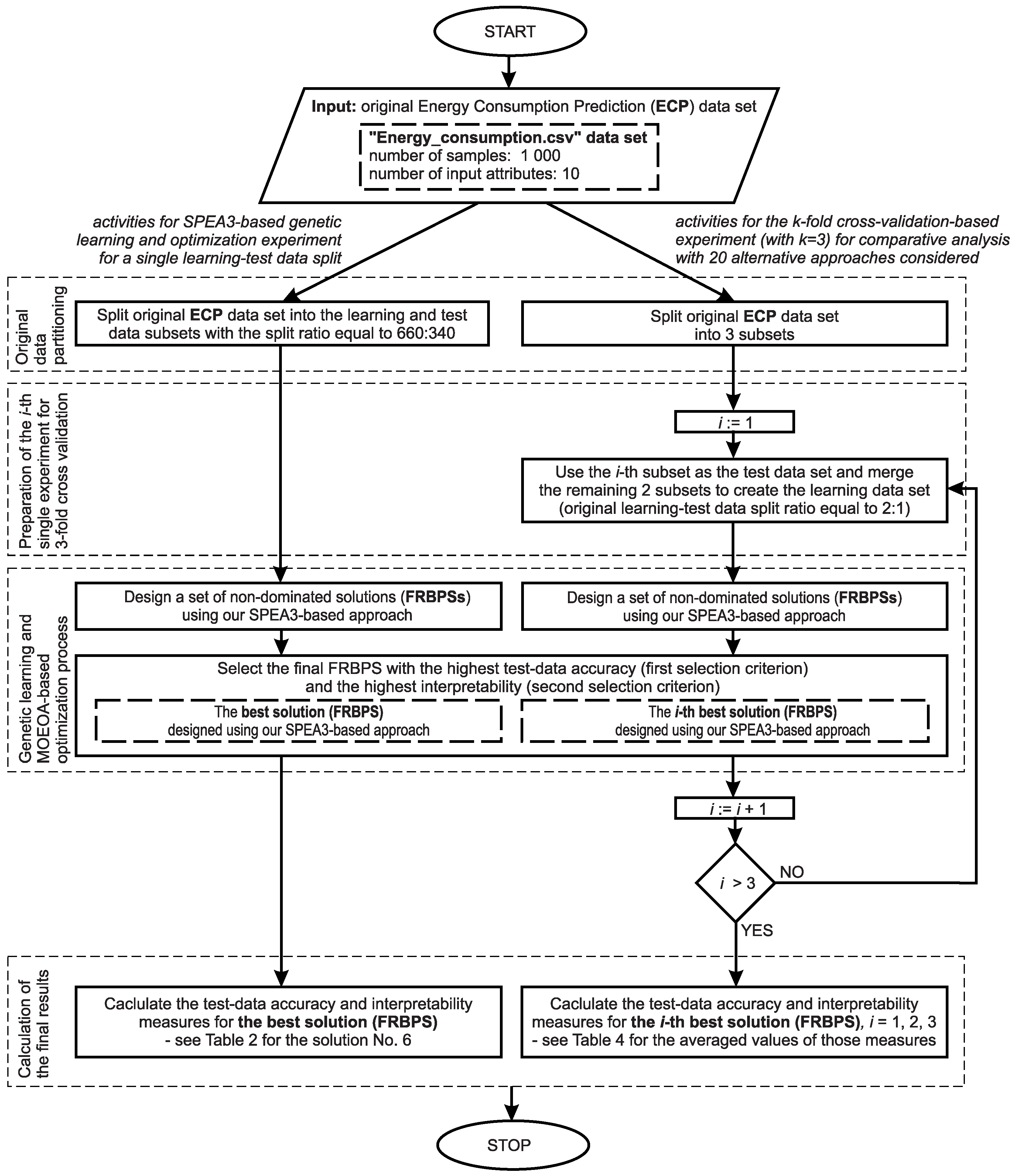
The main part of experiment evaluating our approach consists in performing its cross-validation-based verification. However, before the cross-validation-based experiments are performed and presented, we demonstrate some details of the operation of our approach during the process of the FRBPS designing from data. For this reason, the SPEA3-MOEOA-based genetic learning and optimization experiment for a single learning test data split is presented and discussed. The split ratio of the original data, according to comments of [5], is 660:340. Figure 4 presents a flowchart showing sequences of activities implementing our methodology for both groups of experiments. These activities include, in general, the partitioning of the original data set into the learning and test data sets, the genetic learning and optimization process, and the calculation of the accuracy and interpretability measures of the solutions (FRBPSs) obtained.
Figure 5 presents a 10-element collection (front) of non-dominated solutions (optimized FRBPSs) generated in a single run of our FRBPS designing technique. Each solution is characterized in Figure 5 by its complexity measure Q C P L X (15) as well as its accuracy measures, Q R M S E ( l r n ) (13) in the learning data set and Q R M S E ( t s t ) in the test data set ( Q R M S E ( t s t ) is calculated for the test data in an analogous way to Q R M S E ( l r n ) for the learning data). The collection of Figure 5 represents the best available approximations of Pareto-optimal solutions generated by our approach. The considered collection of solution begins with solution No. 1 (of highest interpretability and lowest accuracy) and ends with the solution No. 10 (of lowest interpretability and highest accuracy in the learning data set). Particular solutions from the considered collection are characterized by different levels of optimized accuracy–interpretability trade-off. Therefore, the user can select a single solution (a specific FRBPS represented by its knowledge base) characterized by a desired level of trade-off between its accuracy and interpretability.
In principle, the user’s choice can be made in any way, starting with the FRBPS of highest interpretability (but accepting its typically low accuracy) and ending with the FRBPS of highest overall accuracy in learning and test data sets (but accepting its generally worse interpretability); see such extreme solutions No. 1 and No. 10, respectively, in Figure 5. However, it seems that the FRBR characterized by the highest ability to generalize knowledge, i.e., the FRBPS of the highest accuracy in the test data set (data not seen during the learning process), is the best choice in the first step of the FRBPS selection procedure; see such solution No. 6 in Figure 5. If there are more than one such FRBS (i.e., characterized by the same and highest test-data accuracy), the FRBPS of highest interpretability is chosen out of the earlier-selected FRBPSs—it is the second step of the FRBPS selection procedure. It does not occur in our case since in the first step we selected only one system—the earlier-mentioned solution No. 6.
The numerical details of accuracy and interpretability of all solutions (FRBPSs) from Figure 5 are collected in Table 2, in which n I N P / R is the averaged number of input attributes per rule and Q R M S E ( t s t ) is the root mean square error (RMSE) of our approach in the test data set. It is calculated in an analogous way to Q R M S E ( l r n ) (13). Bearing in mind that our approach is also an interpretability-oriented one, in Table 2, we also include the MAPE (Mean Absolute Percentage Error) accuracy measures for all FRBPSs from Figure 5. The MAPE measure is scale-independent and easier to interpret in comparison with RMSE. The MAPE measure expresses the system response error as a percentage of the desired output response. For the learning data set, it is defined as follows (for the test data set—in an analogous way):
Q M A P E ( l r n ) = 100 % · 1 K k = 1 K y k ( l r n ) y k y k ( l r n ) ;
y k ( l r n ) and y k are the same as in Formula (13). It should be emphasized that MAPE cannot replace RMSE as the optimization objective. MAPE generates undefined errors for y k = 0 and relatively large errors for small y k . The RMSE measure does not have these drawbacks and is universal (it can be used in both classification and regression problems). The remaining parameters in Table 2 are defined in Section 3 of the paper.
Solution No. 6 of Figure 5 and Table 2 characterized by the highest test data accuracy and high interpretability (only five rules with a 3.2 averaged number of input attributes per rule) is of particular interest (see the cross-validation experiment later in this section). Linguistic fuzzy rule bases of solutions (FRBPSs) from Figure 5 and Table 2 are presented in Table 3 (Figure 6 shows membership functions of fuzzy sets used in those rule bases); solution No. 10 of the lowest interpretability (21 rules) is not included in Table 3.
Table 3 reveals an interesting regularity. We can see that the rule base of solution No. 2 contains the one-rule base of solution No. 1 (marked by red font in the rule base of solution No. 2). In turn, the rule bases of solutions Nos. 3 and 4 contain both rules (marked by red font) from the rule base of solution No. 2). Next, the rule base of solution No. 5 contains all three rules (marked by red font; one slightly modified) from the rule base of solution No. 4. In what follows, the rule base of solution No. 6 contains all four rules (marked by red font) from the rule base of solution No. 5, etc. In general, the rule base of solution No. i contains the rule base of solution No. i 1 (marked by red font in Table 3), i = 2 , 3 , , 10 . Therefore, if higher FRBPS accuracy is required, then our approach either introduces some additional fuzzy rules or extends the earlier-discovered rules. In such a way, our approach provides a more detailed (more accurate) description of the prediction problem we consider. It ts worth emphasizing that such a regularity confirms an internal integrity of our approach.
In order to demonstrate some practical aspects regarding FRBPS interpretability, an example based on solution No. 6 from Table 3 is considered. Its five rules can be aggregated into four, easier-to-interpret sentences, in which the technical names of attributes and the labels of fuzzy sets are replaced with more friendly and semantics-related terms:
  • If temperature is small, then energy consumption is slightly smaller than average.
  • If temperature increases slightly but the number of occupants is small and if HVAC and lighting systems are turned off, then energy consumption is still slightly smaller than average (as in the case of rule No. 1).
  • If the lighting system is turned on but the number of occupants is relatively small, the HVAC system is turned off, and renewable energy sources provide a small amount of energy, then energy consumption is still slightly smaller than average (as in the case of rule No. 1).
  • If temperature is still low (as in the case of rule No. 1) but the HVAC system is turned on or the number of occupants is relatively large, then energy consumption increases slightly (in comparison with the case of rule No. 1).
The first and most general rule confirms the quite obvious direct dependence of energy consumption on temperature. The next two rules can be interpreted as a recipe for maintaining low energy consumption in houses with (relatively) few inhabitants, in two cases: (i) when the temperature rises or (ii) when the lighting system is turned on (e.g., in the evenings). In the first case, HVAC and lighting systems should be turned off. In the second case, the HVAC system should be turned off and an additional source of renewable energy (providing at least a small amount of energy) should be turned on to compensate the energy consumption of the lighting system. The last rule indicates the reasons for increased energy consumption despite low temperatures (in comparison with previous rules), i.e., the energy consumption rises when the HVAC system is turned on or a large number of residents live in the house. Naturally, the interpretation of rules for more complex problems (with many input attributes) may not be so obvious as in this example.
The proposed approach has some limitations regarding the interpretability of generated rules. On the one hand, systems with the lowest complexity (top-left extreme part of the Pareto-front approximation) usually contain a very small number of rules with a small number of input attributes. These rules describe quite simple and usually obvious relationships between data. For this reason, they often do not bring anything groundbreaking to the considered regression problem (see, e.g., solution No. 1 in Table 3 indicating only a simple, direct dependence of energy consumption on temperature). On the other hand, systems with very complex structures (bottom-right extreme part of the Pareto-front approximation) contain many rules with a large number of input attributes. Some of them are often of low strength (i.e., they are activated by a small number of data samples) and represent unique, exceptional, and special cases of a given regression problem. Due to the small number of such cases in the learning data set, they cannot be considered as representative ones. Therefore, general conclusions drawn on the basis of rules describing such specific data may be false. Ultimately, the most valuable systems are located in the middle part of the Pareto-front approximation (like the considered solution No. 6 in Figure 5). They contain not very complex rules with relatively high strength and, because of this, they have a high ability to generalize knowledge, which is confirmed by their high accuracy for test data. Drawing conclusions based on such rules and their interpretation is devoid of the above-mentioned shortcomings.
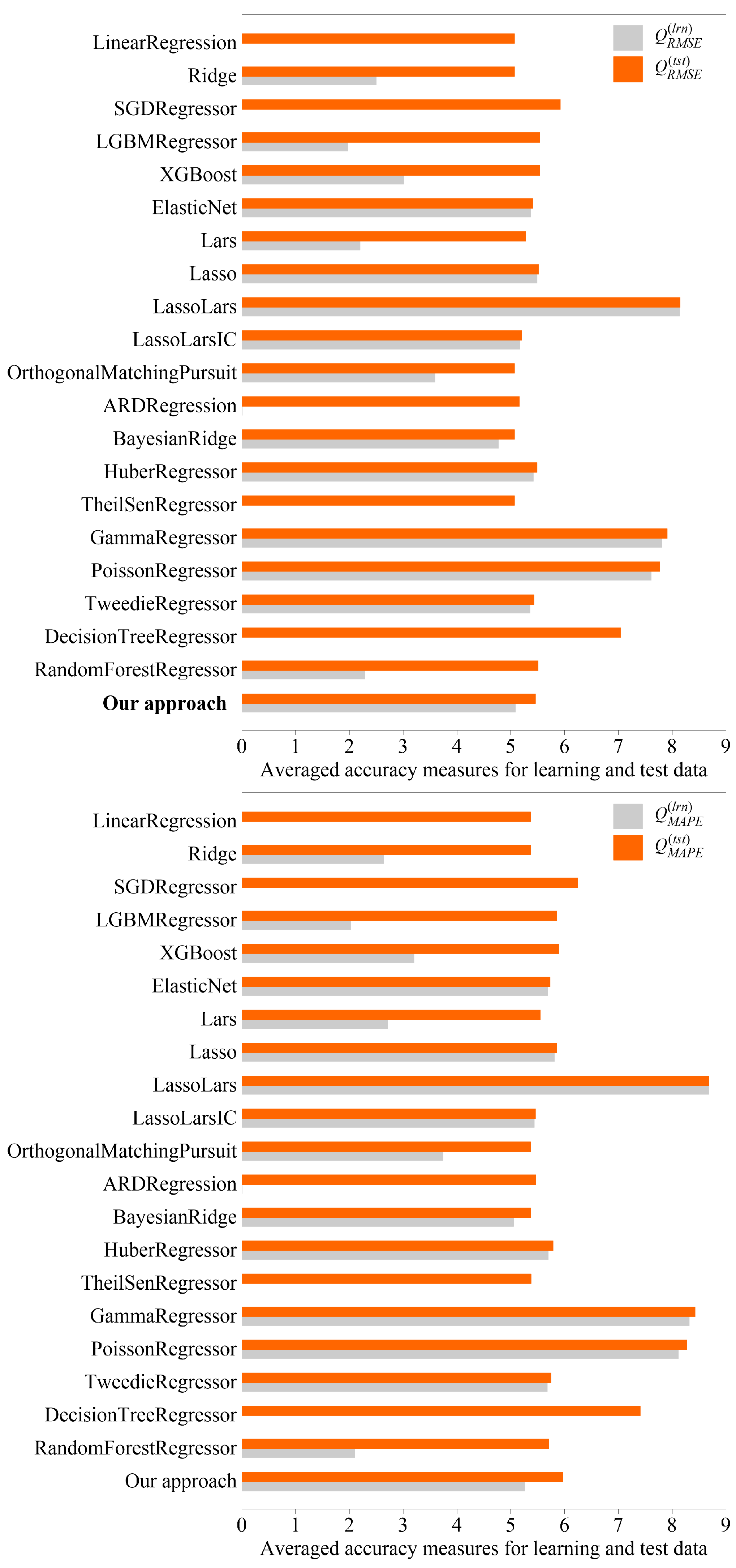
An important part of this work is the cross-validation-based evaluation of our approach. Following the earlier-mentioned original learning test data split ratio equal to 640:340, i.e., roughly equal to 2:1, we performed the k-fold cross-validation experiment with k = 3 (i.e., with 2:1 learning test data split ratio). A single learning experiment begins with generation of a Pareto-front approximation as shown earlier in this section (see Figure 5, Table 2 and Table 3). In turn, a single solution characterized by the highest test data accuracy is selected from that front approximation. If more than one such solutions occur, then one solution characterized by the highest interpretability is selected (it is solution No. 6 in Figure 5, Table 2 and Table 3). Next, the results from all k = 3 partial experiments are averaged. Such an experiment is then repeated 10 times for different initializations of our approach. The final averaged results are shown in the last row of Table 4, which also collects the averaged results of as many as 20 alternative methods applied to the considered data set. The results of Table 4 are presented in the form of “mean value ± standard deviation” except for n I N P ¯ for non-rule-based systems which operate on all 10 input attributes; in such cases, n I N P ¯ = n I N P = 10 . For reader convenience, the results of Table 4 (the mean values of averaged accuracy and interpretability measures) are also presented in a graphical form (using horizontal bar graphs) in Figure 7 and Figure 8.
We consider six groups of alternative approaches. The first group, referred to as “Clasical linear regressors”, includes (i) ordinary least squares linear regression (in brackets, we offer the corresponding software implementation name; see [48]; in the considered case—LinearRegression), (ii) linear least squares with L2 regularization (Ridge), (iii) linear model fitted by minimizing a regularized empirical loss using Stochastic Gradient Descent, SGD (SGDRegressor), (iv) Light Gradient Boosting Model (LGBMRegressor), and (v) eXtreme Gradient Boosting for regression (XGBoost). The second group, labeled “Regressors with variable selection”, includes (i) linear regression with combined L1 and L2 priors as a regularizer (ElasticNet), (ii) Least Angle Regression model, LARS (Lars), (iii) linear model trained with L1 prior as regularizer (Lasso), (iv) Lasso model fit with LARS (LassoLars), (v) Lasso model fit with LARS applying Bayes Information Criterion or Aikake Information Criterion for model selection (LassoLarsIC), and (vi) orthogonal matching pursuit model (OrthogonalMatchingPursuit). The third group of “Bayesian regressors” covers (i) Bayesian Automatic Relevance Determination, ARD, regression (ARDRegression), and (ii) Bayesian Ridge regression (BayesianRidge). The fourth group of “Outlier-robust regressors” includes (i) L2-regularized linear regression model that is robust to outliers (HuberRegressor) and (ii) Theil-Sen estimator: robust multivariate regression model (TheilSenRegressor). The fifth group of “Generalized linear models (GLM) for regression” covers (i) a generalized linear model with a Poisson distribution (PoissonRegressor), (ii) a generalized linear model with a Tweedie distribution (TweedieRegressor), and (iii) a generalized linear model with a Gamma distribution (GammaRegressor). The sixth and last group of “Decision trees and random forests” includes (i) decision trees (DecisionTreeRegressor) and (ii) random forests (RandomForestRegressor). The DecisionTreeRegressor, RandomForestRegressor, LGBMRegressor, and XGBoost methods of Table 4 can process only numerical attributes. For this reason, each categorical attribute of the considered data set is converted to a i binary numerical attributes ( a i is the number of “values” of the ith categorical attribute; see Section 3 of this work); as a result of that, the overall number of input attributes processed by those four methods increases from 10 to 18.
The overwhelming majority of the alternative techniques of Table 4 are the black-box, non-transparent, and non-interpretable approaches focusing only on prediction accuracy. Also, the four earlier-mentioned and rule-generating methods can be included in the black-box class of methods since they generate huge numbers (hundreds) of complex rules. Therefore, all alternative methods are favored, in a way, with regard to our approach, which aims at optimizing the accuracy–interpretability trade-off of prediction systems. However, despite that, the proposed method generates the predictions that are not only highly accurate but also highly interpretable (i.e., using, on average, only 5.3 fuzzy rules with 3.3 input attributes per rule). Concluding, the approach we propose significantly outperforms alternative methods in terms of interpretability of the energy consumption predictions made while remaining comparable or slightly superior in terms of the accuracy of those predictions.

6. Conclusions

The problem of an accurate as well as interpretable and transparent prediction of energy consumption in residential buildings is considered in this paper. The solution that we propose in this work to address the considered problem employs the knowledge discovery machine learning approach combining fuzzy systems with evolutionary optimization. The proposed approach is characterized by both high accuracy and high interpretability and transparency or, more specifically, igenetically optimized accuracy–interpretability trade-off of generated predictions. The trade-off optimization is carried out by means of multi-objective evolutionary optimization algorithms. For that purpose, we use our generalization of the well-known strength Pareto evolutionary algorithm 2 (SPEA2). The accuracy (i.e., the ability to make correct predictions) and the interpretability and transparency (i.e., the ability to formulate compact, explicit, and understandable explanations of mechanisms governing those predictions) are important features of many prediction systems including energy consumption predictions. Fuzzy linguistic rules are characterized by easy-to-grasp interpretation and comprehensibility. Compact sets of such rules generated by our approach belong to the most effective knowledge representation schemes in various domains, including the domain of energy consumption prediction. The most recently published in [5] energy consumption prediction data set is used in the reported experiments.
The contribution of this work includes both methodology and experimental investigations. From the methodological point of view, the designing procedure of fuzzy rule-based prediction systems proposed in this work is our original extension and generalization (for regression problems operating on continuous outputs) of our approach to designing fuzzy rule-based classifiers (operating on discrete outputs, i.e., class labels), which we developed earlier and recently published in this journal in [10]. The experimental contribution of this work includes designing the collection of fuzzy rule-based prediction systems characterized by optimized accuracy–interpretability trade-off levels for residential building energy consumption prediction. The earlier-mentioned and most recently published in [5] data set was used in those experiments. A comparison of our approach with 20 available alternative methods shows that our approach significantly outperforms alternative methods in terms of interpretability and transparency of the energy consumption predictions made while remaining comparable or slightly superior in terms of the accuracy of those predictions.
Our future research will concentrate on improving the effectiveness of algorithms for the optimization of system accuracy–interpretability trade-off. Such algorithms are essential in designing highly accurate and highly interpretable modern classification and regression systems from data in various areas of applications including electricity consumption prediction. Such systems can be classified as explainable artificial intelligence systems (see, e.g., [49,50]) or interpretable machine learning systems (see, e.g., [51,52]).

Author Contributions

Conceptualization, M.B.G. and F.R.; Methodology, M.B.G. and F.R.; Software, M.B.G. and F.R.; Validation, M.B.G. and F.R.; Formal analysis, M.B.G. and F.R.; Investigation, M.B.G. and F.R.; Resources, M.B.G. and F.R.; Data curation, M.B.G. and F.R.; Writing—original draft, M.B.G. and F.R.; Writing—review & editing, M.B.G. and F.R.; Visualization, M.B.G. and F.R.; Supervision, M.B.G. and F.R. All authors have read and agreed to the published version of the manuscript.

Funding

This research received no external funding. No APC (this is the waiver paper).

Data Availability Statement

Data supporting reported results can be found at https://www.kaggle.com/datasets/mrsimple07/energy-consumption-prediction/data; see also [5] for comments.

Conflicts of Interest

The authors declare no conflict of interest.

References

  1. Seem, J. Using intelligent data analysis to detect abnormal energy consumption in buildings. Energy Build. 2007, 39, 52–58. [Google Scholar] [CrossRef]
  2. Spertino, F.; Leo, P.D.; Cocina, V. Which are the constraints to the photovoltaic grid-parity in the main European markets? Sol. Energy 2014, 105, 390–400. [Google Scholar] [CrossRef]
  3. Zhao, P.; Suryanarayanan, S.; Simoes, M. An energy management system for building structures using a multi-agent decision-making control methodology. IEEE Trans. Ind. Appl. 2013, 49, 322–330. [Google Scholar] [CrossRef]
  4. Candanedo, J.; Dehkordi, V.; Stylianou, M. Model-based predictive control of an ice storage device in a building cooling system. Appl. Energy 2013, 111, 1032–1045. [Google Scholar] [CrossRef]
  5. MrSimple07. Energy-Consumption-Prediction. 2024. Available online: https://www.kaggle.com/dsv/7436840 (accessed on 15 April 2024).
  6. Samuel, A.L. Some Studies in Machine Learning Using the Game of Checkers. IBM J. Res. Dev. 1959, 3, 210–229. [Google Scholar] [CrossRef]
  7. What Is Computational Intelligence? Available online: https://cis.ieee.org/about/what-is-ci (accessed on 15 April 2024).
  8. Dubois, D.; Prade, H. What are fuzzy rules and how to use them. Fuzzy Sets Syst. 1996, 84, 169–185. [Google Scholar] [CrossRef]
  9. Fazzolari, M.; Alcala, R.; Nojima, Y.; Ishibuchi, H.; Herrera, F. A review of the application of multiobjective evolutionary fuzzy systems: Current status and further directions. IEEE Trans. Fuzzy Syst. 2013, 21, 45–65. [Google Scholar] [CrossRef]
  10. Gorzałczany, M.B.; Piekoszewski, J.; Rudziński, F. A Modern Data-Mining Approach Based on Genetically Optimized Fuzzy Systems for Interpretable and Accurate Smart-Grid Stability Prediction. Energies 2020, 13, 2559. [Google Scholar] [CrossRef]
  11. Khalil, M.; McGough, A.; Pourmirza, Z.; Pazhoohesh, M.; Walker, S. Machine Learning, Deep Learning and Statistical Analysis for forecasting building energy consumption—A systematic review. Eng. Appl. Artif. Intell. 2022, 115, 105287. [Google Scholar]
  12. Klyuev, R.; Morgoev, I.; Morgoeva, A.; Gavrina, O.; Martyushev, N.; Efremenkov, E.; Mengxu, Q. Methods of Forecasting Electric Energy Consumption: A Literature Review. Energies 2022, 15, 8919. [Google Scholar] [CrossRef]
  13. Al-Shargabi, A.; Almhafdy, A.; Ibrahim, D.; Alghieth, M.; Chiclana, F. Buildings’ energy consumption prediction models based on buildings’ characteristics: Research trends, taxonomy, and performance measures. J. Build. Eng. 2022, 54, 104577. [Google Scholar] [CrossRef]
  14. Han-Yun, C.; Ching-Hung, L. Electricity consumption prediction for buildings using multiple adaptive network-based fuzzy inference system models and gray relational analysis. Energy Rep. 2019, 5, 1509–1524. [Google Scholar]
  15. Zheng, S.; Xu, H.; Mukhtar, A.; Hizam Md Yasir, A.S.; Khalilpoor, N. Estimating residential buildings’ energy usage utilising a combination of Teaching-Learning-Based Optimization (TLBO) method with conventional prediction techniques. Eng. Appl. Comput. Fluid Mech. 2023, 17, 2276347. [Google Scholar] [CrossRef]
  16. Fayaz, M.; Kim, D. A Prediction Methodology of Energy Consumption Based on Deep Extreme Learning Machine and Comparative Analysis in Residential Buildings. Electronics 2018, 7, 222. [Google Scholar] [CrossRef]
  17. Nsangou, J.C.; Kenfack, J.; Nzotcha, U.; Salomon, P.; Ekam, N.; Voufo, J.; Tamo, T.T. Explaining household electricity consumption using quantile regression, decision tree and artificial neural network. Energy 2022, 250, 123856. [Google Scholar] [CrossRef]
  18. Lazzari, F.; Mor, G.; Cipriano, J.; Gabaldon, E.; Grillone, B.; Chemisana, D.; Solsona, F. User behaviour models to forecast electricity consumption of residential customers based on smart metering data. Energy Rep. 2022, 8, 3680–3691. [Google Scholar] [CrossRef]
  19. Adegoke, M.; Hafiz, A.; Ajayi, S.; Olu-Ajayi, R. Application of Multilayer Extreme Learning Machine for Efficient Building Energy Prediction. Energies 2022, 15, 9512. [Google Scholar] [CrossRef]
  20. Aliev, R.; Kacprzyk, J.; Pedrycz, W.; Jamshidi, M.; Babanli, M.; Sadikoglu, F. (Eds.) Prediction of Energy Consumption in Residential Buildings Using Type-2 Fuzzy Wavelet Neural Network; Lecture Notes in Networks and Systems; Springer: Cham, Switzerland, 2023; Volume 610. [Google Scholar]
  21. Chujie, L.; Sihui, L.; Zhengjun, L. Building energy prediction using artificial neural networks: A literature survey. Energy Build. 2022, 262, 111718. [Google Scholar]
  22. Olu-Ajayi, R.; Alaka, H.; Sulaimon, I.; Sunmola, F.; Ajayi, S. Building energy consumption prediction for residential buildings using deep learning and other machine learning techniques. J. Build. Eng. 2022, 45, 103406. [Google Scholar] [CrossRef]
  23. Lei, L.; Wei, C.; Bing, W.; Chao, C.; Wei, L. A building energy consumption prediction model based on rough set theory and deep learning algorithms. Energy Build. 2021, 240, 110886. [Google Scholar] [CrossRef]
  24. Wei, C.; Xiaodong, W.; Chaoen, L.; Jingjing, S.; Jianguo, X. Predicting the energy consumption in buildings using the optimized support vector regression model. Energy 2023, 273, 127188. [Google Scholar]
  25. Khajavi, H.; Rastgoo, A. Improving the prediction of heating energy consumed at residential buildings using a combination of support vector regression and meta-heuristic algorithms. Energy 2023, 272, 127069. [Google Scholar] [CrossRef]
  26. Deng, H.; Fannon, D.; Eckelman, M. Predictive modeling for US commercial building energy use: A comparison of existing statistical and machine learning algorithms using CBECS microdata. Energy Build. 2018, 163, 34–43. [Google Scholar] [CrossRef]
  27. Olu-Ajayi, R.; Alaka, H.; Sulaimon, I.; Sunmola, F.; Ajayi, S. Machine learning for energy performance prediction at the design stage of buildings. Energy Sustain. Dev. 2022, 66, 12–25. [Google Scholar] [CrossRef]
  28. Pandarasamy, A.; Kameshwar, P.; Clayton, M. BEEM: Data-driven building energy benchmarking for Singapore. Energy Build. 2022, 260, 111869. [Google Scholar]
  29. Dinmohammadi, F.; Han, Y.; Shafiee, M. Predicting Energy Consumption in Residential Buildings Using Advanced Machine Learning Algorithms. Energies 2023, 16, 3748. [Google Scholar] [CrossRef]
  30. Anam Nawaz, K.; Naeem, I.; Rashid, A.; Do-Hyeun, K. Ensemble Prediction Approach Based on Learning to Statistical Model for Efficient Building Energy Consumption Management. Symmetry 2021, 13, 405. [Google Scholar] [CrossRef]
  31. Priyadarshini, I.; Sahu, S.; Kumar, R.; Taniar, D. A machine-learning ensemble model for predicting energy consumption in smart homes. Internet Things 2022, 20, 100636. [Google Scholar] [CrossRef]
  32. Guimei, W.; Azfarizal, M.; Hossein, M.; Nima, K.; Quynh, T. Application and evaluation of the evolutionary algorithms combined with conventional neural network to determine the building energy consumption of the residential sector. Energy 2024, 298, 131312. [Google Scholar]
  33. Mohsen, A.; Soofiabadi, M.; Nikpour, M.; Naderi, H.; Abdullah, L.; Arandian, B. Developing a Deep Neural Network with Fuzzy Wavelets and Integrating an Inline PSO to Predict Energy Consumption Patterns in Urban Buildings. Mathematics 2022, 10, 1270. [Google Scholar] [CrossRef]
  34. Lize, W.; Dong, X.; Lifeng, Z.; Zixuan, Z. Application of the hybrid neural network model for energy consumption prediction of office buildings. J. Build. Eng. 2023, 72, 106503. [Google Scholar]
  35. Suqin, X.; Yang, L.; Qiuyang, L.; Zhishan, Y.; Somayeh, P. Energy consumption prediction by modified fish migration optimization algorithm: City single-family homes. Appl. Energy 2024, 353, 122065. [Google Scholar]
  36. Moldovan, D.; Slowik, A. Energy consumption prediction of appliances using machine learning and multi-objective binary grey wolf optimization for feature selection. Appl. Soft Comput. 2021, 111, 107745. [Google Scholar] [CrossRef]
  37. Seyedzadeh, S.; Rahimian, F.P.; Oliver, S.; Glesk, I.; Kumar, B. Data driven model improved by multi-objective optimisation for prediction of building energy loads. Autom. Constr. 2020, 116, 103188. [Google Scholar] [CrossRef]
  38. Mystakidis, A.; Koukaras, P.; Tsalikidis, N.; Ioannidis, D.; Tjortjis, C. Energy Forecasting: A Comprehensive Review of Techniques and Technologies. Energies 2024, 17, 1662. [Google Scholar] [CrossRef]
  39. Cordón, O.; Herrera, F.; Hoffman, F.; Magdalena, L. Genetic Fuzzy Systems: Evolutionary Tuning and Learning of Fuzzy Knowledge Bases; Advances in Fuzzy Systems—Applications and Theory; World Scientific: Singapore, 2001; Volume 19. [Google Scholar]
  40. Herrera, F. Genetic fuzzy systems: Taxonomy, current research trends and prospects. Evol. Intell. 2008, 1, 27–46. [Google Scholar] [CrossRef]
  41. Baczyński, M.; Jayaram, B. Fuzzy Implications; Studies in Fuzziness and Soft Computing; Springer: Berlin/Heidelberg, Germany, 2008. [Google Scholar]
  42. Gorzałczany, M.B. Computational Intelligence Systems and Applications: Neuro-Fuzzy and Fuzzy Neural Synergisms; Studies in Fuzziness and Soft Computing; Physica-Verlag: New York, NY, USA, 2002. [Google Scholar]
  43. Gacto, M.J.; Alcala, R.; Herrera, F. Interpretability of linguistic fuzzy rule-based systems: An overview of interpretability measures. Inf. Sci. 2011, 181, 4340–4360. [Google Scholar] [CrossRef]
  44. Zitzler, E.; Laumanns, M.; Thiele, L. SPEA2: Improving the strength Pareto evolutionary algorithm for multi-objective optimization. In Proceedings of the Evolutionary Methods for Design, Optimization and Control with Applications to Industrial Problems, Barcelona, Spain, 19–21 September 2001; pp. 95–100. [Google Scholar]
  45. Rudziński, F. Finding sets of non-dominated solutions with high spread and well-balanced distribution using generalized strength Pareto evolutionary algorithm. In Proceedings of the 2015 Conference International Fuzzy Systems Association and Europ. Society for Fuzzy Logic and Technology (IFSA-EUSFLAT-15), Gijón, Spain, 30 June–3 July 2015; José, M.A., Humberto, B., Marek, R., Eds.; Volume 89, pp. 178–185. [Google Scholar]
  46. Gorzałczany, M.B.; Rudziński, F.; Piekoszewski, J. Business Intelligence in Airline Passenger Satisfaction Study—A Fuzzy-Genetic Approach with Optimized Interpretability-Accuracy Trade-Off. Appl. Sci. 2021, 11, 5098. [Google Scholar] [CrossRef]
  47. Miller, G. The magical number seven plus or minus two: Some limits on our capacity for processing information. Psychol. Rev. 1956, 63, 81–97. [Google Scholar] [CrossRef]
  48. Pedregosa, F.; Varoquaux, G.; Gramfort, A.; Michel, V.; Thirion, B.; Grisel, O.; Blondel, M.; Prettenhofer, P.; Weiss, R.; Dubourg, V.; et al. Scikit-learn: Machine Learning in Python. J. Mach. Learn. Res. 2011, 12, 2825–2830. Available online: https://scikit-learn.org (accessed on 15 April 2024).
  49. Arrieta, A.B.; Diaz-Rodriguez, N.; Del Ser, J.; Bennetot, A.; Tabik, S.; Barbado, A.; Garcia, S.; Gil-Lopez, S.; Molina, D.; Benjamins, R.; et al. Explainable artificial intelligence (XAI): Concepts, taxonomies, opportunities and challenges toward responsible AI. Inf. Fusion 2020, 58, 82–115. [Google Scholar] [CrossRef]
  50. Samek, W.; Montavon, G.; Vedaldi, A.; Hansen, L.; Müller, K.R. (Eds.) Explainable AI: Interpreting, Explaining and Visualizing Deep Learning; Lecture Notes in Artificial Intelligence; Springer Nature Switzerland AG: Cham, Switzerland, 2019. [Google Scholar]
  51. Monar, C. Interpretable Machine Learning. A Guide for Making Black Box Models Explainable. Under the Creative Commons Attribution-NonCommercial-ShareAlike 4.0 International License. 2020, pp. 1–318. Available online: https://christophm.github.io/interpretable-ml-book/ (accessed on 15 April 2024).
  52. Escalante, H.J.; Escalera, S.; Guyon, I.; Baró, X.; Güçlütürk, Y.; Güçlü, U.; Gerven, M. (Eds.) Explainable and Interpretable Models in Computer Vision and Machine Learning; The Springer Series on Challenges in Machine Learning; Springer Nature Switzerland AG: Cham, Switzerland, 2018. [Google Scholar]
Figure 1. S-type, M-type, and L-type fuzzy sets with Gaussian-like membership functions and their parameters; see (1)–(3).
Energies 17 03242 g001
Figure 2. Illustration of the implementation of the strong fuzzy partition (SFP) requirements for the three-set SFP of the v domain for Gaussian-like membership functions.
Energies 17 03242 g002
Figure 3. Initial shapes of membership functions of 7 fuzzy sets (linguistic terms) describing each numerical attribute.
Energies 17 03242 g003
Figure 4. Sequences of activities implementing our methodology for (i) the SPEA3-based genetic learning and optimization experiment for a single learning test data split (the left branch of the flowchart) and (ii) the k-fold cross-validation-based experiment (with k = 3 ) for comparative analysis with 20 alternative approaches considered (the right branch of the flowchart).
Energies 17 03242 g004
Figure 5. The best Pareto-front approximations generated by our approach.
Energies 17 03242 g005
Figure 6. Final shapes of membership functions of numerical input and output attributes occurring in fuzzy rule bases of Table 4.
Energies 17 03242 g006aEnergies 17 03242 g006b
Figure 7. Graphical presentation of averaged accuracy measures (mean values) for learning and test data from Table 4.
Energies 17 03242 g007
Figure 8. Graphical presentation of averaged interpretability measures (mean values) from Table 4 (except for averaged number of fuzzy sets n F S , which occur only in our approach).
Energies 17 03242 g008
Table 1. Details of particular records of the data set used in our experiment.
No. Attribute NameAttribute TypeAttribute DomainAttribute Description
1.input attributesTimestampdate, time[1 January 2022,
11 February 2022]
The chronological record of each data point, providing a time-based context.
2.Temperaturenumerical-real[20, 30]Randomly generated values representing ambient temperatures in degrees Celsius.
3.Humiditynumerical-real[30, 60]Randomly generated values reflecting the humidity level as a percentage.
4.SquareFootagenumerical-real[1000, 2000]Simulated values representing the size of the environment in square footage.
5.Occupancynumerical-integer[0, 9]Randomly generated integer values indicating the number of occupants.
6.HVACUsagecategoricalOn, OffCategorical variable denoting the HVAC system’s operational state (‘On’ or ‘Off’).
7.LightingUsagecategoricalOn, OffCategorical variable indicating the lighting system’s operational state (‘On’ or ‘Off’).
8.RenewableEnergynumerical-real[0.01, 30]Randomly generated values representing the contribution of renewable energy sources as a percentage.
9.DayOfWeekcategoricalMonday, …, SundayCategorical variable indicating the day of the week.
10.HolidaycategoricalYes, NoCategorical variable denoting whether the day is a holiday (‘Yes’ or ‘No’).
11.output attributeEnergy Consumptionnumerical-real[53.2, 99.2]Output (target) attribute.
Table 2. The accuracy and interpretability measures of solutions from Figure 5.
No.Objective Function ComplementsMAPE-Based Accuracy MeasuresInterpretability Measures
Q CPLX Q RMSE ( lrn ) Q RMSE ( tst ) Q MAPE ( lrn ) Q MAPE ( tst ) R n INP n FS n INP / R
1.0.00625.8415.9736.25%6.38%1121
2.0.08105.7065.6376.14%6.12%2241.5
3.0.08025.4545.5515.95%6.09%3251.3
4.0.12195.2695.4985.50%6.06%3351.3
5.0.22035.1425.4945.31%6.04%4482.2
6.0.31175.0735.4595.24%5.96%55113.2
7.0.40214.9565.5205.19%6.02%76163.4
8.0.49424.8755.6005.08%6.10%87223.7
9.0.67684.7915.5924.97%6.06%109314.8
10.0.84984.6245.7184.84%6.14%219496.3
Table 3. Fuzzy rule bases for solutions (FRBPSs) Nos. 1–9 from Figure 5 and Table 2.
No.Fuzzy Prediction Rules
Solution No. 1:
1.IFTemperature is Small THEN EnergyConsumption is Medium2
Solution No. 2:
1.IFTemperature is Small THEN EnergyConsumption is Medium2
2.IFTemperature is Small AND HVACUsage is On THEN EnergyConsumption is Medium4
Solution No. 3:
1.IFTemperature is Small THEN EnergyConsumption is Medium2
2.IFTemperature is Small AND HVACUsage is On THEN EnergyConsumption is Medium4
3.IFTemperature is Medium1 THEN EnergyConsumption is Medium2
Solution No. 4:
1.IFTemperature is Small THEN EnergyConsumption is Medium2
2.IFTemperature is Small AND HVACUsage is On THEN EnergyConsumption is Medium4
3.IFOccupancy is Medium5 THEN EnergyConsumption is Medium4
Solution No. 5:
1.IFTemperature is Small THEN EnergyConsumption is Medium2
2.IFTemperature is Small AND HVACUsage is On THEN EnergyConsumption is Medium4
3.IFTemperature is Small AND Occupancy is Medium5 THEN EnergyConsumption is Medium4
4.IFTemperature is Medium2 AND Occupancy is Small AND HVACUsage is Off AND LightingUsage is Off THEN EnergyConsumption is Medium2
Solution No. 6:
1.IFTemperature is Small THEN EnergyConsumption is Medium2
2.IFTemperature is Small AND HVACUsage is On THEN EnergyConsumption is Medium4
3.IFTemperature is Small AND Occupancy is Medium5 THEN EnergyConsumption is Medium4
4.IFTemperature is Medium2 AND Occupancy is Small AND HVACUsage is Off AND LightingUsage is Off THEN EnergyConsumption is Medium2
5.IFOccupancy is Medium1 AND HVACUsage is Off AND LightingUsage is On AND RenewableEnergy is Small THEN EnergyConsumption is Medium2
Solution No. 7:
1.IFTemperature is Small THEN EnergyConsumption is Medium2
2.IFTemperature is Small AND HVACUsage is On THEN EnergyConsumption is Medium4
3.IFTemperature is Small AND Occupancy is Medium5 THEN EnergyConsumption is Medium4
4.IFTemperature is Medium2 AND Occupancy is Small AND HVACUsage is Off AND LightingUsage is Off THEN EnergyConsumption is Medium2
5.IFOccupancy is Medium1 AND HVACUsage is Off AND LightingUsage is On AND RenewableEnergy is Small THEN EnergyConsumption is Medium2
6.IFTemperature is Small AND Humidity is not Medium5 AND HVACUsage is On AND LightingUsage is On THEN EnergyConsumption is Medium4
7.IFTemperature is Small AND Humidity is Small AND Occupancy is Large AND HVACUsage is On AND RenewableEnergy is Large THEN EnergyConsumption is Large
Solution No. 8:
1.IFTemperature is Small THEN EnergyConsumption is Medium2
2.IFTemperature is Small AND SquareFootage is not Medium2 AND HVACUsage is On THEN EnergyConsumption is Medium4
3.IFTemperature is Small AND Occupancy is Medium5 AND RenewableEnergy is Large THEN EnergyConsumption is Medium4
4.IFTemperature is Medium2 AND SquareFootage is not Large AND Occupancy is Small AND HVACUsage is Off AND LightingUsage is Off AND RenewableEnergy is not Large THEN EnergyConsumption is Medium2
5.IFOccupancy is Medium1 AND HVACUsage is Off AND LightingUsage is On AND RenewableEnergy is Small THEN EnergyConsumption is Medium2
6.IFTemperature is Small AND Humidity is not Medium5 AND HVACUsage is On AND LightingUsage is On THEN EnergyConsumption is Medium4
7.IFTemperature is Small AND Humidity is Small AND Occupancy is Large AND HVACUsage is On AND RenewableEnergy is Large THEN EnergyConsumption is Large
8.IFTemperature is Medium1 AND Humidity is Medium1 AND SquareFootage is not Medium5 THEN EnergyConsumption is Medium3
Solution No. 9:
1.IFTemperature is Small THEN EnergyConsumption is Medium2
2.IFTemperature is Small AND SquareFootage is not Medium2 AND Occupancy is not Medium1 AND HVACUsage is On THEN EnergyConsumption is Medium4
3.IFTemperature is Small AND Occupancy is Medium5 AND RenewableEnergy is Large THEN EnergyConsumption is Medium4
4.IFTemperature is Medium2 AND Humidity is not Medium5 AND SquareFootage is not Large AND Occupancy is Small AND HVACUsage is Off AND LightingUsage is Off AND RenewableEnergy is not Large THEN EnergyConsumption is Medium2
5.IFOccupancy is Medium1 AND HVACUsage is Off AND LightingUsage is On AND RenewableEnergy is Small THEN EnergyConsumption is Medium2
6.IFTemperature is Small AND Humidity is not Medium2 AND SquareFootage is not Small AND LightingUsage is On AND RenewableEnergy is not Medium2 AND DayOfWeek is Friday THEN EnergyConsumption is Medium5
7.IFTemperature is Small AND Humidity is Small AND Occupancy is Large AND HVACUsage is On AND RenewableEnergy is Large THEN EnergyConsumption is Large
8.IFTemperature is Medium2 AND Humidity is Medium4 AND HVACUsage is On AND RenewableEnergy is Medium4 AND DayOfWeek is Tuesday AND Holiday is No THEN EnergyConsumption is Medium2
9.IFTemperature is Small AND Humidity is not Small AND SquareFootage is not Small AND Occupancy is not Large AND HVACUsage is Off AND DayOfWeek is Wednesday AND Holiday is No THEN EnergyConsumption is Small
10.IFHumidity is Medium3 AND Occupancy is Small AND LightingUsage is Off AND RenewableEnergy is Medium2 AND DayOfWeek is not Friday THEN EnergyConsumption is Medium2
Table 4. Results of our approach and comparison with alternative methods (k-fold cross-validation with k = 3 ; averaged values from 10 runs; n/ap stands for not applicable).
No. MethodAveraged Accuracy Measures for Learning and Test DataAveraged Interpretability Measures
Q RMSE ( lrn ) ¯ Q RMSE ( tst ) ¯ Q MAPE ( lrn ) ¯ Q MAPE ( tst ) ¯ R ¯ n INP ¯ n FS ¯ n INP / R ¯
1.Clasical linear regressorsLinearRegression5.5 × 10−12 ± 2.3 × 10−125.07 ± 0.165.38 × 10−12 ± 2.9 × 10−125.37 ± 0.17n/ap10n/apn/ap
2.Ridge2.50 ± 0.025.07 ± 0.162.64 ± 0.025.37 ± 0.17n/ap10n/apn/ap
3.SGDRegressor3.6 × 10−4 ± 1.1 × 10−55.92 ± 0.93.63 × 10−4 ± 3.5 × 10−66.25 ± 0.18n/ap10n/apn/ap
4.LGBMRegressor1.97 ± 0.055.54 ± 0.302.02 ± 0.065.86 ± 0.423046.4 ± 12.815 ± 0.0n/ap7.91 ± 0.52
5.XGBoost3.01 ± 0.095.54 ± 0.303.20 ± 0.115.89 ± 0.43556.4 ± 19.815 ± 0.0n/ap5.87 ± 0.02
6.Regressors with variable selectionElasticNet5.37 ± 0.045.41 ± 0.155.69 ± 0.055.73 ± 0.19n/ap10n/apn/ap
7.Lars2.20 ± 0.065.28 ± 0.212.71 ± 0.095.55 ± 0.25n/ap10n/apn/ap
8.Lasso5.49 ± 0.055.52 ± 0.165.81 ± 0.065.85 ± 0.21n/ap10n/apn/ap
9.LassoLars8.14 ± 0.058.15 ± 0.218.68 ± 0.068.69 ± 0.26n/ap10n/apn/ap
10.LassoLarsIC5.17 ± 0.075.21 ± 0.175.44 ± 0.085.46 ± 0.18n/ap10n/apn/ap
11.Orthogonal-MatchingPursuit3.59 ± 0.025.07 ± 0.173.74 ± 0.025.37 ± 0.16n/ap10n/apn/ap
12.Bayesian regressorsARDRegression9.65 × 10−3 ± 2.8 × 10−35.16 ± 0.197.78 × 10−3 ± 3.4 × 10−35.47 ± 0.20n/ap10n/apn/ap
13.BayesianRidge4.77 ± 0.055.07 ± 0.165.05 ± 0.055.37 ± 0.16n/ap10n/apn/ap
14.Outlier-robust regressorsHuberRegressor5.42 ± 0.065.49 ± 0.255.70 ± 0.065.79 ± 0.28n/ap10n/apn/ap
15.TheilSenRegressor3.3 × 10−12 ± 1.1 × 10−125.07 ± 0.174.01 × 10−12 ± 1.4 × 10−125.38 ± 0.17n/ap10n/apn/ap
16.Generalized linear modelsGammaRegressor7.81 ± 0.647.91 ± 0.568.32 ± 0.728.43 ± 0.51n/ap10n/apn/ap
17.PoissonRegressor7.61 ± 1.047.77 ± 0.818.12 ± 1.148.27 ± 0.81n/ap10n/apn/ap
18.TweedieRegressor5.36 ± 0.065.43 ± 0.135.68 ± 0.065.75 ± 0.16n/ap10n/apn/ap
19.Decision trees and random forestsDecisionTree-Regressor0.0 ± 0.07.04 ± 0.280.0 ± 0.07.41 ± 0.37800.0 ± 0.017.8 ± 0.4n/ap11.7 ± 0.1
20.RandomForest-Regressor2.29 ± 0.035.51 ± 0.282.10 ± 0.035.71 ± 0.35505.2 ± 6.417.9 ± 0.24n/ap10.9 ± 0.24
21. Our approach5.091 ± 0.155.46 ± 0.215.26 ± 0.165.97 ± 0.235.3 ± 0.65.6 ± 0.611.6 ± 0.63.3 ± 0.06
Disclaimer/Publisher’s Note: The statements, opinions and data contained in all publications are solely those of the individual author(s) and contributor(s) and not of MDPI and/or the editor(s). MDPI and/or the editor(s) disclaim responsibility for any injury to people or property resulting from any ideas, methods, instructions or products referred to in the content.