1. Introduction
Energy is the cornerstone of human life. Humankind relies on traditional sources of energy such as fossil fuels, hydropower, and nuclear energy to meet its energy needs, but these methods pose significant environmental challenges. With China’s government pursuing a “dual-carbon” goal and a strategy to establish a power system based on new energy sources, accelerating the transformation of the energy structure has become particularly urgent. In this context, the development of new energy sources, especially photovoltaic (PV) power generation [
1], has become an important task at present. Although photovoltaic power plants are competitive with traditional fossil fuel power plants, the volatility of solar radiation and the fluctuation of power generation due to various climatic and geographic factors still pose a challenge to the performance of solar power plants and power grids [
2]. Therefore, accurate prediction of PV power becomes the key to solving this problem, which can effectively avoid all the adverse effects caused by the discrepancy between the actual PV power and the expected one.
Predicting PV power involves many complex variables, making it crucial to comprehensively consider these factors when building the prediction model and to employ suitable modelling techniques to achieve the most accurate results possible [
3]. In the early days, machine learning models were used to predict PV power. They are able to learn laws and patterns from data, enabling automated decision making and prediction. Compared to traditional rule coding methods, machine learning is adaptive and can be adapted and optimised to new data, discovering hidden patterns and correlations in the data, which improves the accuracy of the prediction. Random Forest [
4] is an integrated learning method that improves accuracy by building multiple decision trees and combining their predictions. Differential Integration Moving Average Autoregressive Model (ARIMA) [
5] is an autoregressive model that combines difference, integration, and moving average for the modelling and forecasting of time series data. XGBoost [
6] is a gradient boosting algorithm that improves the accuracy and generalisation of a model by integrating multiple weak classifiers (usually decision trees). Support Vector Regression (SVR) [
7] is a regression method based on support vector machines that fit the data by maximising the boundaries and is suitable for dealing with small samples and nonlinear and high-dimensional data. Machine learning algorithms are more efficient in dealing with some simple prediction problems, but historical PV power generation data are usually a multidimensional, nonlinear dataset containing a large number of time steps, whereas neural networks are more expressive and generalisable in dealing with complex, nonlinear problems. Long Short-Term Memory (LSTM) [
8] is a Recurrent Neural Network (RNN) variant suitable for processing and predicting time series data with memory units that capture long-term dependencies. Gated Recurrent Unit (GRU) [
9] is an LSTM-like variant of RNN with update gates and reset gates for capturing long-term dependencies in sequential data more efficiently. Convolutional Neural Network (CNN) [
10] is a neural network used to process input data with a grid structure to extract and learn features through convolutional and pooling layers. BP Neural Networks (Backpropagation Neural Networks) [
11] is a traditional neural network structure that optimises the network parameters by means of backpropagation algorithms for problems such as classification and regression. Deep Belief Networks [
12] are neural networks consisting of multiple layers of constrained Boltzmann machines that learn the distribution and feature representation of data through unsupervised pre-training and supervised fine-tuning.
In the past few years, the Transformer model [
13,
14,
15] has injected new vigour into short-term PV power prediction, mainly in terms of its powerful sequence processing ability and efficient parallel computing capability. Through the self-attention mechanism, Transformer is able to capture remote dependencies and complex nonlinear patterns, thus improving prediction accuracy. In addition, its flexible architecture can easily integrate multiple input features with high adaptability, which improves the model’s performance in handling multivariate prediction. These advantages enable Transformer to demonstrate significant improvements and innovations in the field of PV power prediction. The literature [
16] proposes a Dual Encoder Transformer Model (DualET) that extracts information from image and sequence data by means of wavelet transform and sequence decomposition modules and introduces an attention module to learn the association between temporal features and cloud information. The experimental results of this model on real datasets show that it outperforms other models in short-term PV power prediction.
Due to the volatility and randomness of PV power generation, the accuracy of directly predicting its power is not high. For this reason, the power of PV power generation can be decomposed and each component can be predicted separately to improve the accuracy of the overall prediction. The literature [
17] combines sequence decomposition methods and deep learning models to propose a hybrid model (VMD-GA-Conv-A-LSTM) that can significantly improve the accuracy of PV power prediction. The model first decomposes the PV power sequences using VMD with optimised parameters. It then inputs the sub-sequences with preprocessed historical meteorological data into the LSTM model combining 1D convolution and an attention mechanism for prediction, and obtains the overall prediction value by accumulating the prediction results of each sub-sequence, which shows the best prediction performance on several benchmark models.
A single neural network is prone to overfitting, and intelligent optimisation algorithms can optimise the parameters of the neural network, improve its generalisation ability, reduce its sensitivity to noise, and better handle complex and nonlinear data, thus improving the accuracy and stability of PV power prediction. The literature [
18] applies the Artificial Fish Schooling Algorithm (AFSA) to optimise the BP neural network, leveraging AFSA’s global optimisation and intrinsic parallel computing capabilities to effectively optimise the network’s weights and thresholds, so as to train an efficient PV output power prediction model. The literature [
19] proposes a prediction of a short-term model for PV power using Pearson’s correlation coefficient, EEMD, sample entropy, SSA, and LSTM, and the experimental results demonstrate that the model achieves a low prediction error for PV power under diverse weather conditions. The literature [
20] introduces a system for predicting PV power using a deep convolutional neural network (CNN) coupled with a signal decomposition algorithm. This system extracts deep features using AlexNet for transfer learning, decomposes historical power signals into sub-components, and converts all input parameters into 2D feature maps for CNN input. The literature [
21] introduces ADAMS, a new Autoformer model designed for short-term PV power forecasting. ADAMS utilises a multiscale framework and de-stationary attention mechanism. ADAMS outperforms baselines in predicting PV output.
Based on the above, the previous literature has typically used only one of the methods of decomposing raw PV data or intelligent optimisation algorithms when optimising short-term PV power prediction models, which have limited improvement in prediction accuracy. Therefore, this paper proposes a new model, the SSA-VMD-Informer model, which utilises both approaches and aims to improve the prediction accuracy of short-term PV power. The process is outlined as follows:
Firstly, Informer, a model that uses a self-attentive mechanism with a multilevel temporal prediction mechanism and focuses on processing long series data, is adopted and the temporal coding of the original Informer model is optimised.
Secondly, Variational Mode Decomposition (VMD) is optimised with the intelligent optimisation algorithm Sparrow Search Algorithm (SSA), which automatically adjusts the key parameters of VMD and decomposes the original PV power generation data with the optimal parameters obtained.
Finally, the modal components obtained from the SSA-optimised VMD of the original PV power and other environmental factors affecting PV power generation are inputted into the Informer model, and the reliability and superiority of the model are verified by the PV power generation test.
3. Model Design
3.1. SSA-VMD-Informer Short-Term PV Power Prediction Model
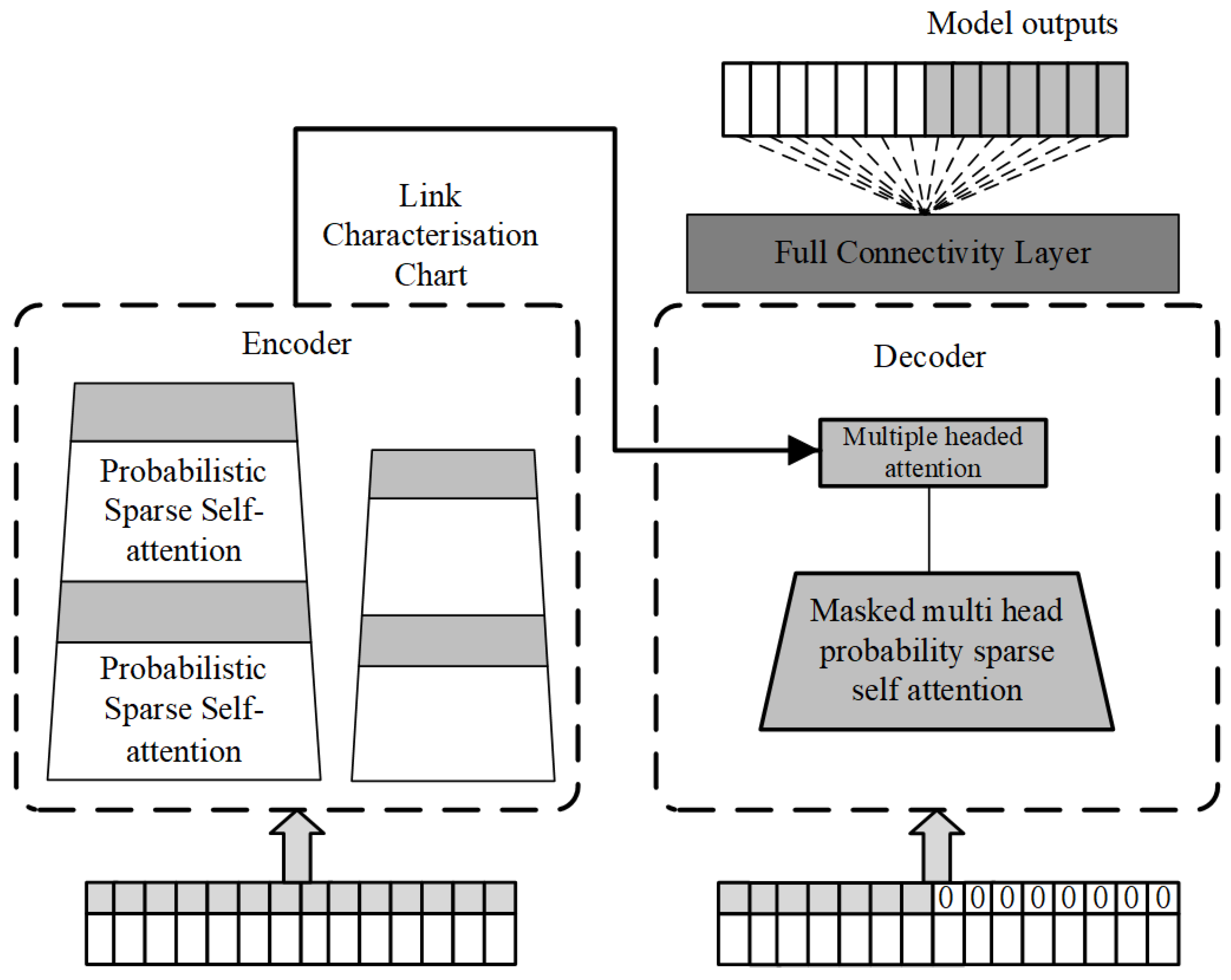
The traditional Transformer model depends on the self-attention mechanism and has demonstrated strong prediction ability in time series, but there are still some problems: the self-attention mechanism needs to evaluate the similarity between a certain moment and all other moments during the calculation process, which leads to higher time complexity; for long sequence data, in order to deal with these data, it is often necessary to use multiple parallel multihead attention structures, which takes up a lot of memory resources; in addition, when using the Transformer model, the prediction speed is reduced when dealing with long sequences because the decoder needs to rely on the output of the previous encoder when making predictions. In this regard, this paper proposes an SSA-VMD-Informer short-term PV power prediction model. This model captures information in time series data more comprehensively, thereby enhancing prediction accuracy. In this paper, the prediction model will be constructed from the following aspects:
Improvements are made to the temporal coding of the Informer model to improve the model’s ability to understand and process time series data.
Decomposition of raw PV power data using variational modal decomposition techniques, which provides support for more in-depth data analysis and processing by increasing the dimensionality of the data.
SSA is introduced to optimise VMD to ensure that VMD can achieve the best decomposition, thus improving the efficiency and effectiveness of data processing.
The components obtained from the SSA-VMD decomposition, as well as the set of relevant factor features of the raw PV power data, are inputs into the improved time-coded Informer model for prediction.
The model structure is shown in
Figure 5.
3.2. Improvement of Informer Time Code
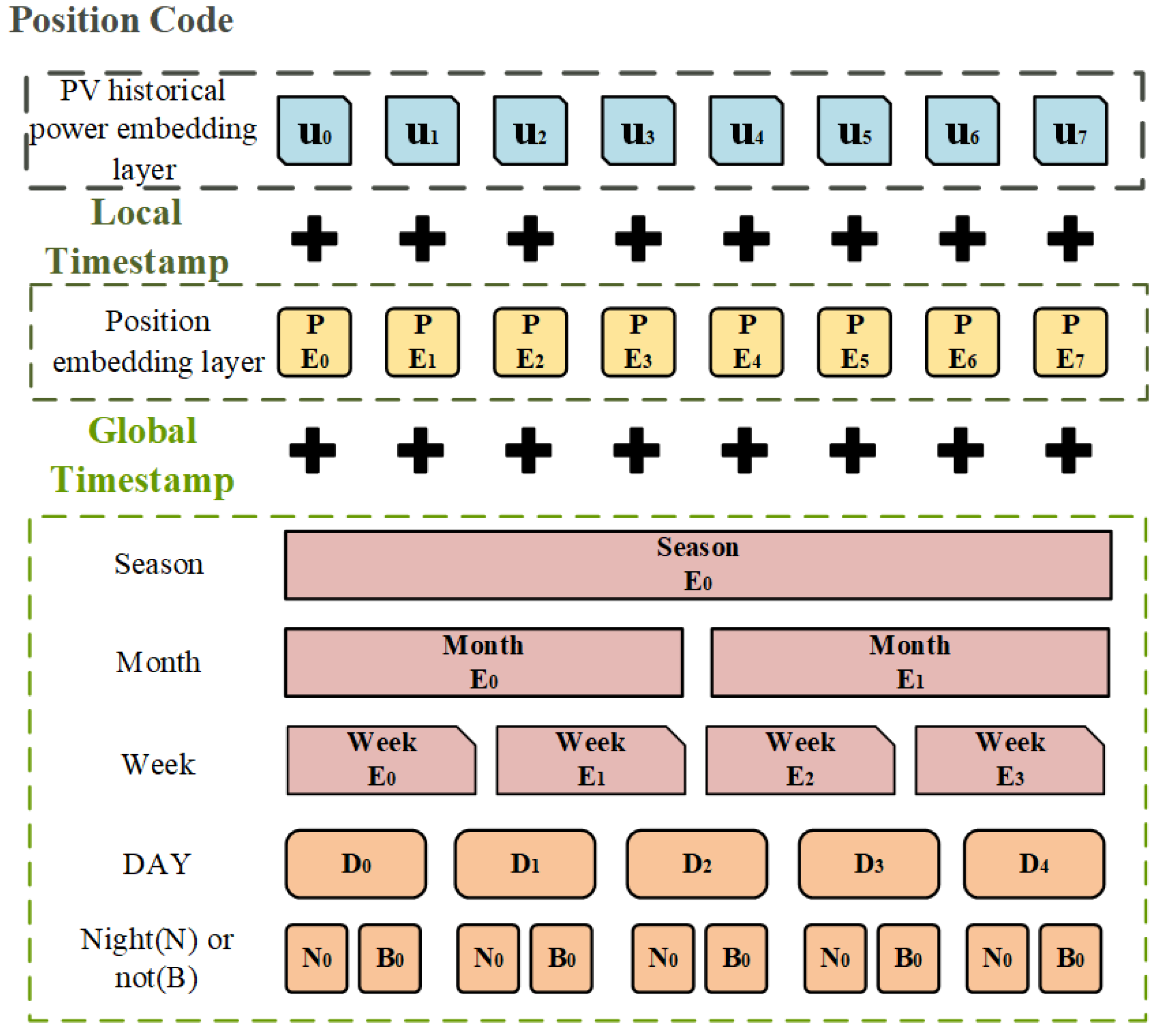
In long sequence timing modelling problems, it is necessary to consider not only local timing information, but also hierarchical timing information, such as day of the week, month, and year, as well as timestamped information for unexpected events such as holidays.
As shown in
Figure 6, the original Informer model location embedding is divided into three types: feature vector, local timestamp (location encoding in Transformer), and global timestamp. The global timestamp part contains week, month, and holiday parts.
In photovoltaic power generation, the amount of power generated is greatly influenced by panel temperature and radiation levels. Panel temperatures follow a descending order from winter to summer and radiation levels follow a descending order from winter to autumn. Hence, the global timestamps for PV power forecasts should include the seasons of each PV’s historical power, along with weeks, months, and holidays.
The PV power mainly depends on the light intensity, so according to the sunrise and sunset time of each month in the area where the PV power plant is located, the PV historical power generation is divided into night and day. The PV power generation data used in this study are from the power generation of the PV power plant in Xinjiang for one year. For example, the sunrise time in January in Xinjiang is about 9:30 and the sunset time is about 19:00, so the data from 0:00 to 9:30 and 19:00 to 24:00 are coded as night, while the data from 19:00 to 24:00 are coded as night and 9:30 to 19:00 are coded as day. The improved time coding is shown in
Figure 7.
The location coding of the Informer model is shown in Equation (11).
where
PE represents the position encoding,
denotes the absolute position of the vector,
denotes the total dimension of the vector,
i denotes the
i-th dimension in the vector, and each dimension in the position encoding has its corresponding sinusoidal signal.
3.3. Intelligent Optimisation Algorithm Selection
The primary objective of an intelligent optimisation algorithm is to locate a solution within the search space that minimises or maximises the value of the fitness function, contingent upon the problem’s characteristics. The fitness function maps a solution x in the problem space to a real value that represents the degree of merit of that solution, the fitness value. The case of lower fitness is usually referred to as a minimisation problem, while higher fitness is usually referred to as a maximisation problem.
In the case of a minimisation problem, the fitness function represents the objective or cost of the problem and the task of the optimisation algorithm is to find the solution that minimises the fitness function. Therefore, when the fitness is lower, it means that the solution is closer to the optimal solution of the problem or better. Optimising VMD with an intelligent optimisation algorithm is a minimisation problem.
We selected the first 10 days of data of raw PV power of the Xinjiang PV power plant in 2019 as an example for VMD and decomposed VMD optimised by three different commonly used optimisation algorithms with minimum sample entropy as the fitness function. The parameters for the intelligent optimisation algorithm are as follows: a maximum of 20 iterations, a population size of 15, and a dimensionality of 2 ( and K). Here, represents the regularisation parameter, which controls the smoothing degree of the signals and the stability of the decomposition results, while K indicates the number of modal functions to be decomposed.
The VMD of different intelligent optimisation algorithms are compared with the optimised VMD of SSA and the trend of the fitness value curves of different optimisation algorithms is obtained, as shown in
Figure 8. The figure shows that SSA achieves its lowest fitness value of 0.049073 in the initial iteration, while WOA and GWO reach the lowest in the third iteration and PSO reaches the lowest in the seventh iteration.
After SSA optimisation, the parameters of VMD are
and
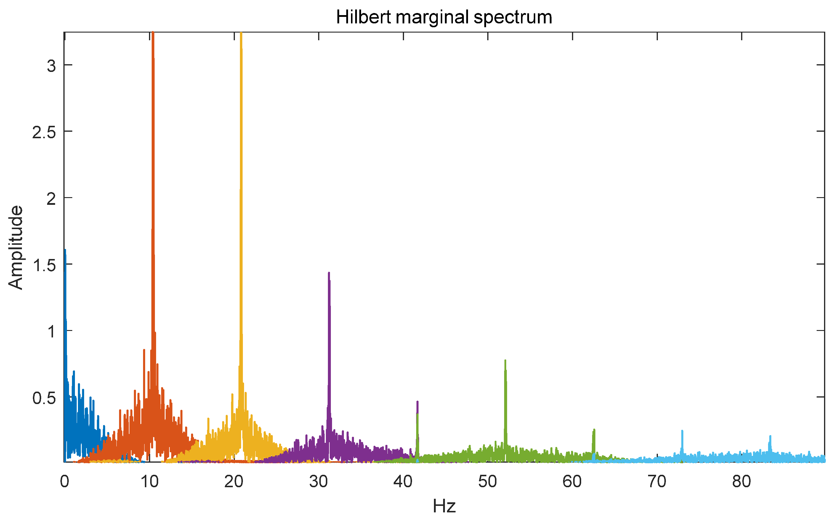
. According to
Figure 9, the nine modal components generated by SSA-VMD decomposition are clearly distinguished in frequency. Each component not only retains the characteristics of the original PV power sequence, but also effectively inhibits mode aliasing. Thus, optimising VMD with SSA enhances the accuracy of PV power prediction.
Therefore, this research component will optimise the parameters of VMD by means of the sparrow optimisation algorithm, with a view to obtaining a combination of the VMD parameters that is more suitable for PV power data, thus improving the performance of the prediction model. This approach is expected to be advantageous in the application of VMD to provide more accurate and reliable decomposition results for PV power prediction.
3.4. SSA Optimisation VMD
In order to optimise VMD using the SSA, we minimise the Sample Entropy (SampEn) as a fitness function. In this case, the key parameters of VMD are the modal number K and the penalty parameter α. These parameters need to be optimised by SSA to minimise the sample entropy:
Firstly, the formula for defining the sample entropy is as in Equation (12). Assuming that the intrinsic modal functions (IMFs) obtained after VMD are
, we weight and sum the sample entropy of each IMF as the total sample entropy.
where
A(
IMF) is the number of pairs of sequences that satisfy the specified similarity metric and
B(
IMF) is the number of pairs of sequences that satisfy the slightly relaxed condition.
In order to make VMD optimal with respect to the parameters
K and α, we define the optimisation objective function as Equation (13).
In this formulation, SSA will optimise with the objective of finding the parameters K and α that minimise the total sample entropy.
The steps to optimise VMD using sparrow optimisation algorithm are:
Initialisation population: generate an initial population containing multiple sparrow individuals, where each sparrow individual represents a set (K, α).
Fitness calculation: for each sparrow individual, decompose the signal using VMD and calculate the sample entropy of each IMF, where the sum is used as the fitness value.
Updating sparrow location: according to the update rule of SSA, update the parameter (K, α) for each sparrow individual so that its fitness value decreases gradually.
Iteration process: Repeat the process of fitness calculation and position updating until the maximum number of iterations is reached or the convergence condition is satisfied.
Output result: finally output the sparrow individual with the smallest fitness value, i.e., the optimal K and α parameters.
By this method, the global search capability and local search accuracy of SSA can be effectively utilised to optimise the VMD parameter settings, thus improving the decomposition quality and computational efficiency.
4. Experiment and Analysis
4.1. Experimental Data and Evaluation Criteria
In this study, short-term PV power prediction experiments are conducted using the measured PV power data from the Xinjiang PV power plant for the year 2019. The dataset consists of 35,041 sets of data with a sampling interval of 15 min. The data include seven meteorological data items, namely, component temperature, temperature, barometric pressure, humidity, total radiation, direct radiation, scattered radiation at the sampling moment, and the corresponding historical data of PV power generation. There are 34,945 sets of data used for model training and the prediction test is carried out on the remaining 96 sets of data.
To analyse the predictive effectiveness of the model developed in this paper and other models,
RMSE,
MAE,
SDE, and
R2 are used to compare and analyse the prediction results, with the formulas expressed as follows.
where
and
are the predicted and true values of the
i-th sampling point, respectively,
t represents the number of prediction steps,
is the mean of the dependent variable, and
n is the sample size.
RMSE can reflect the overall average error of the model’s predicted values.
MAE—Mean Absolute Error; the smaller the
MAE, the more stable the model.
SDE reflects the stability or uncertainty of the sample mean estimation of a set of data, which is a measure of the deviation between the predicted and true values in the PV power generation prediction evaluation indexes; the smaller the
SDE, the more stable the model is.
R2 can help to assess the accuracy of a PV power prediction model; the larger the
R2, the stronger the model’s predictive ability, and conversely the weaker the model’s predictive ability.
4.2. Model Parameter Setting
The main parameters of the Informer model are shown in
Table 1.
4.3. Validation of Time Code Validity
To validate the performance of the improved Informer model with time coding, a comparison is made between the predicted values of the original Informer model, the predicted values of the improved time-coded Informer model, and the true values.
In
Figure 10, the horizontal coordinates represent the number of forecast steps. Since the time resolution of the dataset is 15 min, each step represents 15 min. The horizontal coordinate ranges from 0 to 96, which means it covers a whole day. (The horizontal coordinates of the subsequent prediction curves are the same as here.) From
Figure 10 and
Table 2, it can be seen that after improving the time coding for the PV power data, the predicted values obtained by the Informer network are closer to 0 in the black part of the left and right sides, and the original Informer model’s prediction of the PV power exists below 0, which is not in line with the real situation, while the Informer model with the improved time coding does not have such a problem, and the predicted values are closer to the real values. The RMSE of the improved Informer model decreases by 0.0012, the MAE value decreases by 0.0367, and the SDE value remains unchanged compared to that before the improved time coding, while the R² value increases by 0.0001. It shows that the improved time coding Informer model is more capable of predicting the short-term PV power.
Due to the characteristics of the dataset, the PV power generation dataset of a place in Xinjiang used in this study has a generation value at night that is basically 0. Therefore, in this study, most of the predicted values at night are close to 0 or slightly higher than 0. If the generation value at night in the dataset used is not 0, the model is able to make the corresponding predictions as well.
4.4. VMD and SSA Ablation Study
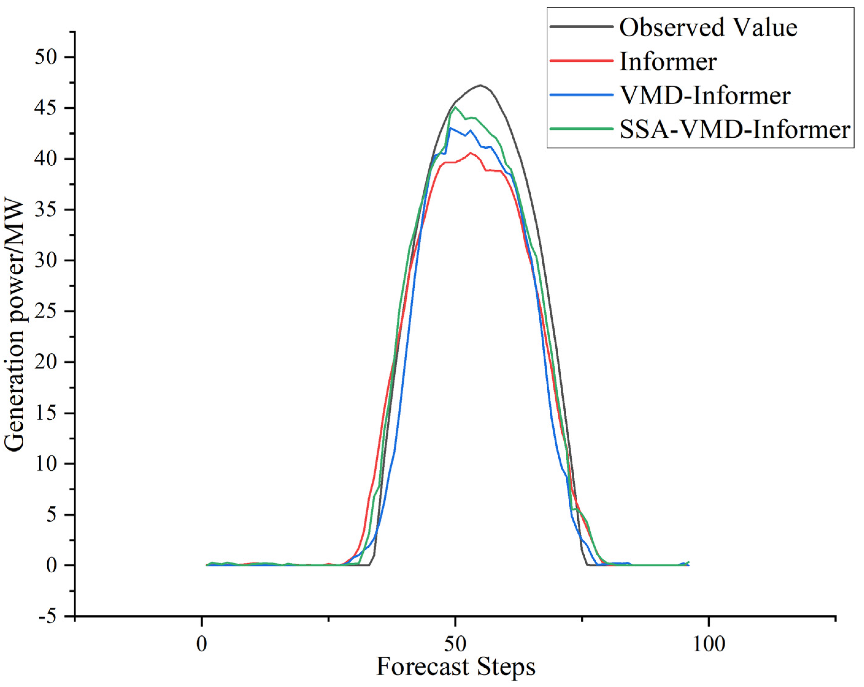
In order to verify whether VMD as well as SSA can improve the capability of the Informer model, the Informer predictions, VMD-Informer predictions, and SSA-VMD-Informer predictions are compared with the true values.
From
Figure 11 and
Table 3, it can be seen that the RMSE of the model with VMD of the raw PV power generation data is reduced by 0.0167, MAE is reduced by 0.0941, SDE is reduced by 0.06, and R
2 is improved by 0.0004. The model with SSA-VMD decomposition of the raw PV power generation data has a reduction of RMSE by 0.718, MAE by 0.1743, and SDE by 0.29, compared to the model decomposed with only VMD, which has a reduction of RMSE by 1.342, MAE by 0.7748, SDE by 0.84, and R
2 by 0.0223. This suggests that VMD and SSA improve model performance.
4.5. Comparative Experiments with Other Models
To validate the superior predictive ability of the SSA-VMD-Informer model, the commonly used classical prediction models LSTM, BiGRU-attention, and Transformer model were selected for prediction comparison experiments.
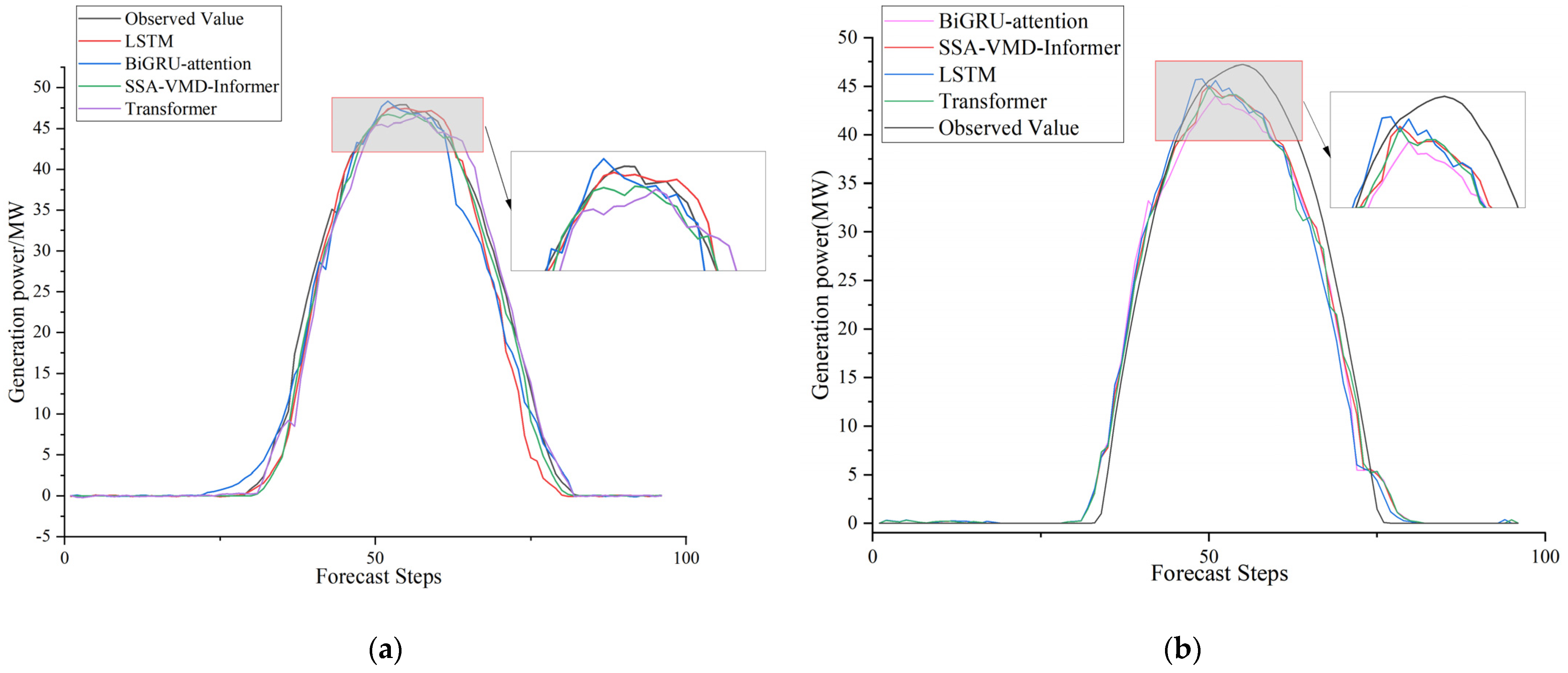
To verify the model’s stability, we chose two random days for PV power prediction: 24 April in spring and 20 October in autumn. By comparing the model’s predictions on these two days with the actual observations, we are able to evaluate the model’s performance under different time conditions. Specifically, if the model’s prediction results on these two different days are able to better match the actual situation, it shows that the model is highly stable and reliable. Such a validation method can effectively reveal the robustness of the model in the face of different input data and ensure its feasibility in practical applications.
As can be seen from the prediction curves in
Figure 12, on 24 April and 20 October, the SSA-VMD-Informer model’s prediction curves align significantly better with the actual value curves compared to other models. The smaller error between the predicted and observed values of the SSA-VMD-Informer model during these two different time periods indicates that the model has higher accuracy and stability in capturing the trend of PV power changes. In contrast, the prediction curves of the other models exhibit large fluctuations and deviations, which indicate their deficiencies in fitting the actual data. Further, through the comparative analysis in
Table 4 and
Table 5, we can clearly see that the prediction results of the SSA-VMD-Informer model on 24 April and 20 October are excellent in all error indicators. Specifically, the RMSE, MAE, and SDE of the model for these two dates are lower than those of other comparative models, and R
2 is higher than those of other comparative models, which indicates that the SSA-VMD-Informer model possesses higher accuracy and reliability in short-term PV power prediction.
