Comparison of Power Coefficients in Wind Turbines Considering the Tip Speed Ratio and Blade Pitch Angle

Abstract

This paper presents a review of the power and torque coefficients of various wind generation systems, which involve the real characteristics of the wind turbine as a function of the generated power. The coefficients are described by mathematical functions that depend on the trip speed ratio and blade pitch angle of the wind turbines. These mathematical functions are based on polynomial, sinusoidal, and exponential equations. Once the mathematical functions have been described, an analysis of the grouped coefficients according to their function is performed with the purpose of considering the variations in the trip speed ratio for all the coefficients based on sinusoidal and exponential functions, and with the variations in the blade pitch angle. This analysis allows us to determine the different coefficients of power and torque used in wind generation systems, with the objective of developing algorithms for searching for the point of maximum power generated and for the active control of wind turbines with variations in the blade pitch angle.

1. Introduction

The progressive growth in global electricity demand results in a deterioration of the environment, which manifests in higher emissions of carbon dioxide (CO₂) and an increase in the greenhouse effect. This is mainly due to the fact that this energy demand has mostly been met by fossil fuels (oil, coal, etc.) [1,2]. The high dependence on fossil fuels, their involvement in “climate change”, and the progressive increase in their costs has motivated interest in other alternative forms of electricity generation that do not depend on fossil fuels [3]. These alternative forms are known as renewable energy sources, and they have led to a diversification of energy generation [4,5]; these new forms include wind energy and solar energy. The wind is a clean and inexhaustible resource that is available in most parts of the world; however, there are specific areas in which this natural resource is abundant [1,6,7,8]. Different statistical methods have been developed to calculate the average wind speed, the wind energy density, and its load factor for a specific geographic area [9]; this allows for the identification of suitable zones for the installation of wind farms of different MWs and low power systems in the order of kWs. Several projects have helped to increase the production of clean electrical energy. At present, there are numerous projects aiming to start up several wind farms, increasing the production of clean electric energy. Meanwhile, the administrations of several countries have established incentives and subsidies for these projects, to comply with the Kyoto Protocol and achieve a reduction in CO₂ emissions.

The recent advances in wind generation systems (WGS) have led to a reduction in costs, bringing them to highly competitive levels compared to the systems of electric generation using conventional energies (oil, coal, etc.) [10].

The process of converting wind energy to electric power originates from the wind gusts colliding with the blades of a wind turbine, which turns an electric generator because it is interconnected with a gearbox. The electric generator provides electric power that is variable in both amplitude and frequency, which is not suitable for common working loads; in addition, the wind is random in nature, so the amplitude and frequency of voltages provided by the generator vary constantly. In order to condition the variable voltages of the generator and to supply loads with amplitude and frequency values according to the regulations of a given country, electronic power systems are used to carry out this conversion [11,12].

One of the most important parameters for evaluating the performance of a wind turbine is the power coefficient, as established by the International Electrotechnical Commission (IEC) in its recommendation IEC 61400-12-1 [13]. The power coefficient (Cp) refers to the relationship between actual power production and the power available in the ambient wind flowing towards the turbine blades [14]. The power coefficient is one of the parameters that is required to calculate the productive efficiency of wind turbines or wind farms, where parameters such as turbulence, temperature, and air density are also involved; in addition, data science is used to analyze all these parameters and make them more efficient [15,16].

The present paper focuses on the behavior of the different wind turbines that are presented in the literature. The wind turbines analyzed in this work are the horizontal axis and three-blade types, because they are the most commonly found. This paper is structured as follows. It begins by showing the characteristics of a wind turbine in order to establish which are the most important parameters that establish its behavior and cause each turbine to have particular characteristics in the process of converting wind energy. With this, it is established that one of the most significant parameters that differentiates one wind turbine from another is the Power Coefficient. The power coefficient determines the power variation that can be obtained from a wind turbine; it should be noted that each model of wind turbine has its own power coefficient. This paper shows the mathematical functions that are used to represent the behavior of the power coefficient in relation to the specific speed and the angle of attack of the blade, establishing general formulas that allow for a better analysis and comparison of the power coefficients. Finally, a discussion of the review based on the practical cases presented in the literature is carried out; this enables us to establish the limitations and the advantages of each of the power coefficients considered in the analysis. The power coefficient can be used for other analyses of wind generation systems, such as the production efficiency of wind turbines.

2. Power and Torque in a Wind Turbine

The generated power of a wind turbine is stable based on the kinetic energy in the air of a mass object (m), which moves at a speed (v). Therefore, the wind kinetic energy is given by:

$$E_v=\frac{1}{2}m{v}^2$$

(1)

The power of the moving air is obtained from the wind energy, assuming that the wind speed (v_ω) is constant and can be expressed by:

$$P_v=\frac{d{E}_v }{d x}=\frac{1}{2}\dot{m}{v}_{\omega }^2$$

(2)

where $\dot{m}$ is the mass airflow per second. If the air passes through an area $\left(A\right)$ and the density of the air is $\left(\rho \right)$, the mass airflow is expressed by:

$$\dot{m}=\rho A{v}_{\omega }$$

(3)

substituting (3) into (2), we obtain:

$$P_v=\frac{1}{2}\rho A{v}_{\omega }^3$$

(4)

where $A$ is the area covered by the blades of the turbine, and can be expressed by:

$$A=\pi r^2$$

(5)

substituting (5) into (4), we obtain:

$$P_v=\frac{1}{2}\rho \pi r^2{v}_{\omega }^3$$

(6)

However, the wind kinetic energy is not converted in its entirety into mechanical energy. This is because the principle of continuity of the air flow passing through the turbine must be met, where the wind passing through the turbine is braked, so it leaves at a lower speed, but is never equal to zero. In an ideal wind turbine, the amount of kinetic energy of the wind that turns into mechanical energy is 59.25%, which is established in Betz’s law. This maximum conversion value is known as the Betz limit. Therefore, a term is added that relates the power of the wind and the power that can be obtained in the turbine, this relationship is known as the power coefficient ($C_p$). Therefore, the power in the turbine ($P_t$) is expressed by:

$$P_t=\frac{1}{2}{C}_p\rho \pi r^2{v}_{\omega }^3$$

(7)

The power coefficient depends on several factors, among which are the type of turbine, that is, if it is a horizontal or vertical axis type; in the case of a horizontal axis, this also depends on the number of blades, the specific speed or trip speed ratio ($\lambda$), and the blade pitch angle of the turbine $\left(\beta \right)$.

In this way, for the same type of turbine, the power coefficient depends on λ and the blade pitch angle, $C_p\left( \lambda ,\beta \right)$.

The symbol $\lambda$ relates to the tangential velocity of the end of the turbine blade between the wind speed. This is expressed by:

$$\lambda =\frac{r{\omega }_m}{v_{\omega }}$$

(8)

where ${\omega }_m$ is the rotational speed of the turbine.

The power coefficient $C_p$ depends on both $\lambda$ and the type of turbine, as shown in Figure 1. The variation of $C_p$ with respect to β and λ is shown in Figure 2.

The other important parameter involved in the process of converting the energy in the turbine is the torque of the turbine shaft, which is related to the power in the turbine. This relationship is expressed by:

$$P_t=T_t{\omega }_m$$

(9)

substituting (7) into (9) and solving $T_t$, we obtain:

$$T_t=\frac{C_p\rho \pi r^2{v}_{\omega }^3}{2{\omega }_m}$$

(10)

substituting (8) into (10) gives:

$$T_t=\frac{1}{2}\frac{C_p}{\lambda }\rho \pi r^3{v}_{\omega }^2$$

(11)

From (11), the torque coefficient ($C_t$) is established by:

$$C_t=\frac{C_p}{\lambda }$$

(12)

substituting (12) into (11) gives:

$$T_t=\frac{1}{2}{C}_t\rho \pi r^3{v}_{\omega }^2$$

(13)

The variation of $C_t$ with respect to λ and the type of turbine is shown in Figure 3, and the same variation in relation to β and λ is shown in Figure 4.

3. Power Coefficient and Torque Coefficient

In the literature, there are different graphical representations of $C_p$; in some cases, these differ considerably. In the case of commercial wind turbines, manufacturers provide documentation where the $C_p$ behavior graphs are provided. These graphs are used to obtain a mathematical approximation that allows us to understand their behavior in an analytical way. These approximations are carried out by means of optimal numerical methods [18].

From conducting an exhaustive bibliographical review, it was found that the mathematical approximations of the variation in the power coefficient are expressed through three mathematical functions:

• Polynomial functions
• Sinusoidal functions
• Exponential functions

The following section shows all of the potency coefficients found in the literature grouped based on their mathematical function, as well as the parameters of the wind generation system where it is used, in order to establish their main characteristics.

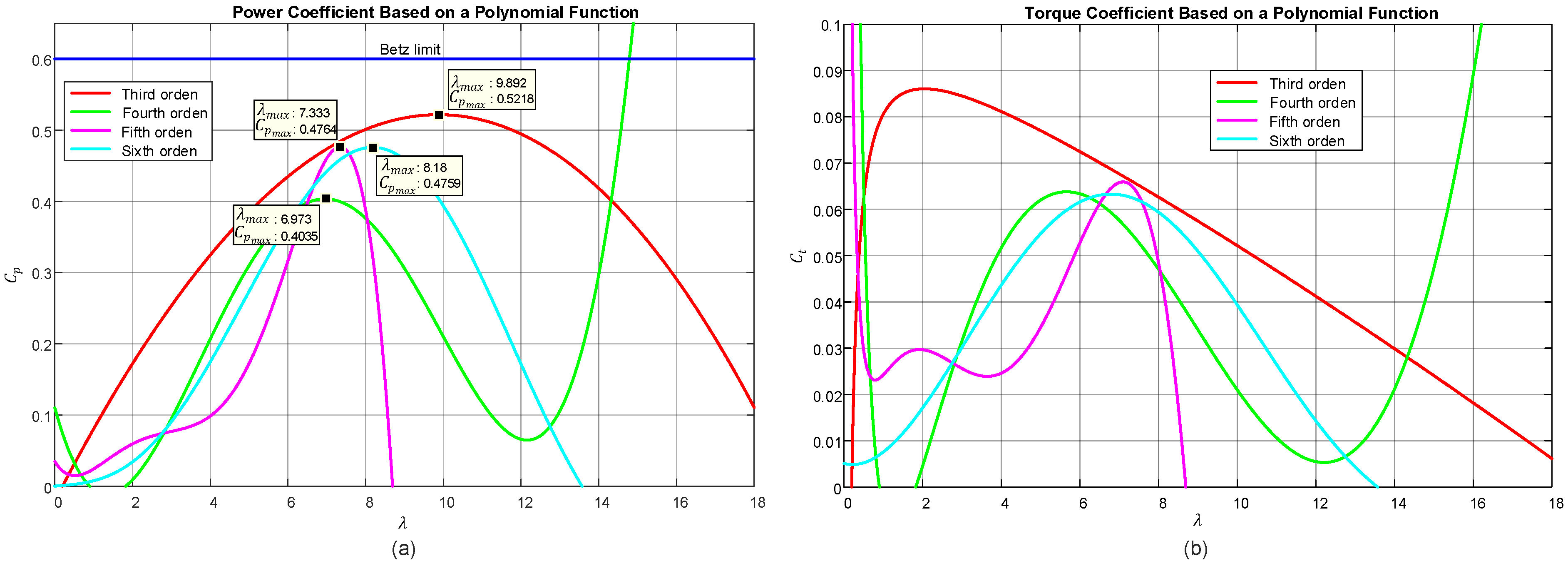
3.1. Polynomial Function

Four power coefficients were found from a review of the literature, and their mathematical expression has the form of a polynomial function. Each of the power coefficients represented by a polynomial equation is detailed below; these are identified by the order of the polynomial. From the bibliographic review, four power coefficients were found, where their mathematical expression has the form of an exponential function. These are identified according to the order of the polynomial function presented by the authors in the paper.

3.1.1. Third-Order Polynomial Function

In [19,20], the authors show the hardware implementation of control algorithms for constant wind speed turbine emulator based on a DC-Machine. This system includes a wind speed profile, a mathematical model of a horizontal axis wind turbine, a separately excited DC-Machine, and a fourth quadrant chopper. The power coefficient only depends on λ and is expressed by:

$$C_p\left(\lambda \right)=-3.7\times {10}^{-5}{\lambda }^3-0.004834{\lambda }^2+0.1063\lambda -0.02086$$

(14)

This power coefficient is used for a wind generation system with a blade radius of 1.086 m, and the system has a power of 3 kW. This paper presents the simulation results in Matlab/Simulink.

3.1.2. Fourth-Order Polynomial Function

In [21,22], the authors present an isolated small wind turbine emulator based on a separately excited DC motor. It was developed to emulate and evaluate the performance of a small wind turbine using different control strategies. The power coefficient only depends on λ and is expressed by:

$$C_p\left(\lambda \right)=0.00044{\lambda }^4-0.012{\lambda }^3+0.097{\lambda }^2-0.2\lambda +0.11$$

(15)

This paper presents experimental results in Matlab/Simulink.

3.1.3. Fifth-Order Polynomial Function

In [23,24], an improved maximum-power-point tracking algorithm for wind-energy conversion systems is presented. The proposed method significantly reduces the turbine mechanical stress related to conventional techniques, so that both the maintenance needs and the medium time between failures are expected to be improved. The power coefficient only depends on λ and is expressed by:

$$C_p\left(\lambda \right)=0.043-0.108\lambda +0.146{\lambda }^2-0.0605{\lambda }^3+0.0104{\lambda }^4-0.0006{\lambda }^5$$

(16)

This power coefficient is used for a wind generation system with a blade radius of 1.525 m and the system has a power of 2 kW. This paper presents simulation and experimental results.

3.1.4. Sixth-Order Polynomial Function

In [25], the authors present a wind turbine emulator (WTE) that is designed and implemented considering different requirements from the development and testing of a control strategy in a doubly fed wind-power-generating system. The power coefficient only depends on λ and is expressed by:

$$\begin{gathered} C_p\left(\lambda \right)=0.051-0.0022\lambda +0.0052{\lambda }^2-5.1425\times {10}^{-4}{\lambda }^3-2.795\times {10}^{-5}{\lambda }^4+4.6313\times {10}^{-6}{\lambda }^5 \\ -1.331\times {10}^{-7}{\lambda }^6 \end{gathered}$$

(17)

This power coefficient is used for a wind generation system with a blade radius of 2.5 m and the system has a power of 4.2 kW. This paper presents experimental results.

3.1.5. General Exponential Function

Based on the general polynomial function shown in [25,26], this is expressed by:

$$C_p\left(\lambda \right)={\displaystyle \sum }_{i=0}^{i=n}{a}_i{\lambda }^i$$

(18)

All the power coefficients based on a polynomial function are grouped according to (18). Considering that the maximum order found in the functions is the sixth, the equation expressed by (19) is obtained. The constants of each polynomial function are shown in

Table 1. Constants of the power coefficients found in relation to the order of the general polynomial function.

Constants	Third	Fourth	Fifth	Sixth
$a_0$	−0.02086	0.11	0.0344	0.0051
$a_1$	0.1063	−0.2	−0.0864	−0.0022
$a_2$	−0.004834	0.097	0.1168	0.0052
$a_3$	−3.7 × 10−5	−0.012	−0.0484	−5.1425 × 10−4
$a_4$	0	0.00044	0.00832	−2.795 × 10−5
$a_5$	0	0	−0.00048	4.6313 × 10−6
$a_6$	0	0	0	−1.331 × 10−7

.

$$C_p\left(\lambda \right)=a_0{\lambda }^0+a_1{\lambda }^1+a_2{\lambda }^2+a_3{\lambda }^3+a_4{\lambda }^4+a_5{\lambda }^5+a_6{\lambda }^6$$

(19)

The behavior of the four power coefficients based on a polynomial function in relation to λ are shown in Figure 5a. The graph indicates the maximum value of the power coefficient ($C_{p_{max}}$), as well as the value of λ for that point (${\lambda }_{max}$), in each of the functions found. None of the coefficients exceed the Betz limit. In the established interval of $\lambda$ between 0 to 18, the $C_p$ of the third, fifth and sixth orders have adequate behavior; however, the fourth-order function must be limited to an $\lambda$ of 12.16 because, for higher values of $\lambda$, the value of $C_p$ begins to increase again, which does not correspond to a real behavior of a wind turbine. The torque coefficient is obtained using (12). Therefore, in Figure 5b, the behavior of the power coefficient in relation to λ is shown, based on polynomial functions of the power coefficient.

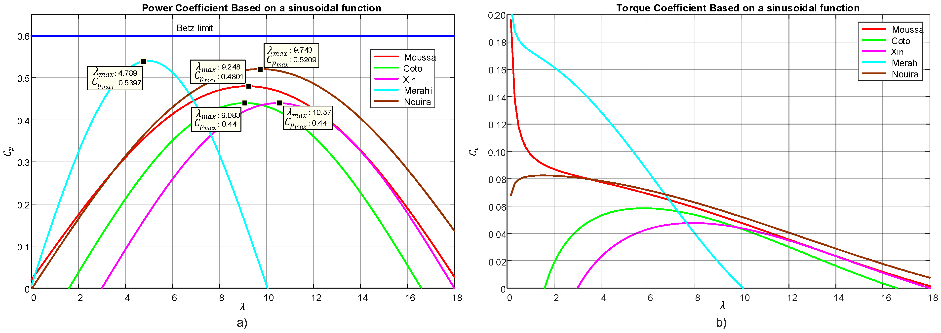
3.2. Sinusoidal Function

From the bibliographic review, five power coefficients were found where their mathematical expressions have the form of a sinusoidal function. Then, each of them is detailed; these are identified by the authors of the paper where the power coefficient was found.

3.2.1. Moussa, Bouallegue, and Kehedher [19]

In [19], the authors show the hardware implementation of control algorithms for a constant wind speed turbine emulator based on a DC-Machine. This system includes the wind speed profile, mathematical model of a horizontal axis wind turbine, a separately excited DC-Machine, and a fourth quadrant chopper. The power coefficient used depends on both λ and β in degrees, and is expressed by:

$$C_p\left(\lambda ,\beta \right)=\left[0.5-0.00167\left(\beta -2\right)\right]\sin \left[\frac{\pi \left(\lambda +0.1\right)}{18.5-0.3\left(\beta -2\right)}\right]+0.00184\left(\lambda -3\right)\left(\beta -2\right)$$

(20)

This power coefficient is used for a wind generation system with a blade radius of 1.086 m and the system has a power of 3 kW. This paper presents simulation results in Matlab/Simulink.

3.2.2. Coto, García, Díaz, and Gómez [27]

In [27], the authors explain the design, implementation, and simulation of a model that represents the possible conditions of wind that can occur in a given wind installation. The power coefficient used depends on both λ and β in degrees, and is expressed by:

$$C_p\left(\lambda \right)=0.44\sin \left[\frac{\pi \left(\lambda -1.6\right)}{15}\right]$$

(21)

This power coefficient is used for a wind generation system with a blade radius of 48.2 m and a power of 750 kW. This paper presents simulation results in Matlab/Simulink.

3.2.3. Xin, Wanli, Bin, and Pengcheng [28]

In [28], the authors propose a sliding-mode variable-structure controller based on the analysis of the feature model of the variable pitch and the speed wind turbine generator system, in order to improve the dynamic performance in the operational areas of constant power output in wind generation system. The power coefficient used depends on both λ and β in degrees and it is expressed by:

$$C_p\left(\lambda ,\beta \right)=\left[0.44-0.0167\beta \right]\sin \left[\frac{\pi \left(\lambda -3\right)}{15-0.3\beta }\right]-0.00184\left(\lambda -3\right)\beta$$

(22)

This power coefficient is used for a wind generation system with a blade radius of 35 m and a power of 2 MW. This paper presents simulation results.

3.2.4. Merahi, Mekhilef, and Madjid [29]

In [29], the authors present the DC-voltage regulation of a five-level neutral-point clamp in a closed loop. It consists of regulating the average value of the DC-voltage by using one loop instead of four loops. The modeling and the control of the different components of the wind energy conversion system are presented. The wind turbine is controlled using the maximum power point tracking algorithm based on the wind speed estimation. The power coefficient used depends on both λ and β in degrees, and is expressed by:

$$C_p\left(\lambda ,\beta \right)=\left[0.5-0.0167\left(\beta -2\right)\right]\sin \left[\frac{\pi \left(\lambda +0.1\right)}{10-0.3\left(\beta \right)}\right]-0.00184\left(\lambda -3\right)\left(\beta -2\right)$$

(23)

This power coefficient is used for a wind generation system with a blade radius of 70.5 m and a power system of 1.5 MW. This paper presents simulation results.

3.2.5. Nouira and Khedher [18]

In [18], the authors present the implementation of an experimental wind energy board using a DC-machine as a wind emulator. The power coefficient used depends on both λ and β in degrees, and is expressed by:

$$C_{pf }\left(\lambda ,\beta \right)=\left[0.5+0.0167\left(\beta -2\right)\right]\sin \left[\frac{\pi \left(\lambda +0.1\right)}{18.5-0.3\left(\beta -2\right)}\right]-0.00184\left(\lambda -3\right)\left(\beta -2\right)$$

(24)

This power coefficient is used for a wind generation system with a blade radius of 20 m and power of 10 kW. This paper presents experimental results.

3.2.6. General Sinusoidal Function

All the power coefficients registered in a sinusoidal function are grouped for general equation purposes based on a sinusoidal function. The general equation is expressed by (25), and the constants of each sinusoidal function are shown in the

Table 2. Constants of the power coefficients found in relation to the general sinusoidal function.

Constants	Moussa	Coto	Xin	Merahi	Nouira
$b_0$	0.5	0.44	0.44	0.5	0.5
$b_1$	−0.00167	0	−0.00167	−0.00167	0.00167
$b_2$	−2	0	0	−2	−2
$b_3$	0.1	−1.6	−3	0.1	0.1
$b_4$	18.5	15	15	10	18.5
$b_5$	−0.3	0	−0.3	−0.3	−0.3
$b_6$	−2	0	0	0	−2
$b_7$	0.00184	0	0.00184	−0.00184	−0.00184
$b_8$	−3	0	−3	−3	−3
$b_9$	−2	0	0	−2	−2

.

$$C_{pf }\left(\lambda ,\beta \right)=\left[b_0+b_1\left(\beta +b_2\right)\right]\sin \left[\frac{\pi \left(\lambda +b_3\right)}{b_4+b_5\left(\beta +b_6\right)}\right]+b_7\left(\lambda +b_8\right)\left(\beta +b_9\right)$$

(25)

The behavior of the five power coefficients based on a sinusoidal function in relation to λ and β equal to zero are shown in Figure 6a. β is equal to zero for the purpose of comparing its behavior with the power coefficients based on a polynomial function, since this does not include β. These coefficients are identified according to the first author of the paper where the power coefficient is presented. The graph indicates the maximum value of the power coefficient ($C_{p_{max}}$), as well as the value of λ for that point (${\lambda }_{max}$), in each of the functions found. None of the coefficients exceed the Betz limit. In the established interval of $\lambda$ between 0 to 18, the $C_p$ values established by Moussa [19], Coto [27], Xin [28] and Nouira [18] have adequate behavior. However, the power coefficient established by Merahi [29] must be limited to a $\lambda$ of 10.05, because, for higher values of $\lambda$, the values of $C_p$ are negative, which does not correspond to a real behavior of a wind turbine. The torque coefficient is obtained using (12). Therefore, in Figure 6b, the behavior of the power coefficient in relation to λ is shown, based on sinusoidal functions of the power coefficient.

To more thoroughly evaluate the power coefficients based on sinusoidal functions, an analysis is conducted with variations of the specific velocity and β.

The behavior of the $C_p$ and $C_t$ proposed by Moussa, Bouallegue, and Kehedher [19], with variations of $\lambda$ and $\beta ,$ is shown by Figure 7. It is observed that, with high β values, abnormal behavior occurs, because $C_p$ increases again after having decreased. On the other hand, the $C_t$ increases considerably when $\beta$ increases, so this coefficient is not recommended for use when implementing control techniques through β.

The behavior of the $C_p$ and $C_t$ proposed by Xin, Wanli, Bin, and Pengcheng [28] with variations of $\lambda$ and $\beta$ is shown in Figure 8. It is observed that the behavior of $C_p$ and $C_t$ is adequate, because, with high β values, the coefficients decrease, so a control through β can be implemented with this proposed coefficient.

The behavior of the $C_p$ and $C_t$ proposed by Merahi, Mekhilef, and Madjid [29] with variations of $\lambda$ and $\beta$ is shown in Figure 9. The behavior of $C_p$ is adequate because, as β increases, the coefficient decreases; however, the same does not happen with $C_t$, because, with low β and high β, the value of $C_t$ increases considerably, which does not allow for control techniques to be applied through β.

The behavior of the $C_p$ and $C_t$ proposed by Nouira and Khedher [18] with variations of $\lambda$ and $\beta$ is shown in Figure 10. The behavior of $C_p$ does not vary considerably with the variation of β; in addition, $C_t$ increases considerably with low β and high blade pitch angles, which does not allow for control techniques to be applied through β.

3.3. Exponencial Function

From the bibliographic review, eight power coefficients were found where their mathematical expression has the form of an exponential function; then, each of them is detailed. These coefficients are identified by the authors of the paper where the power coefficient was found.

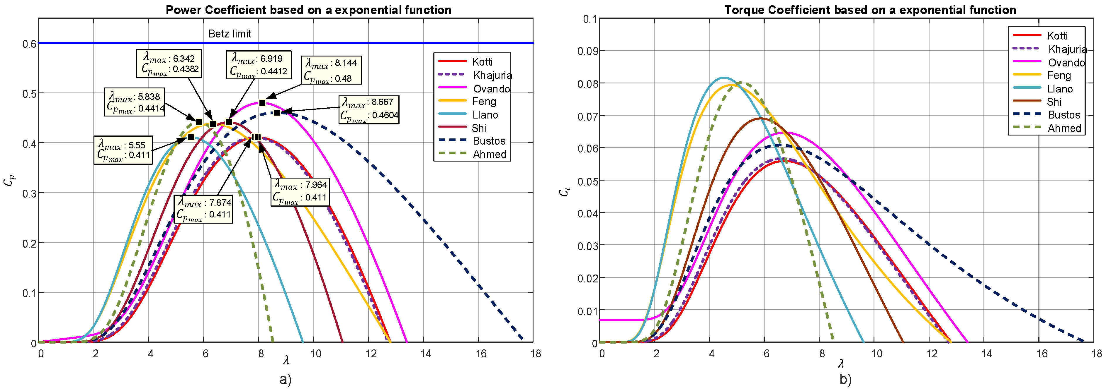
3.3.1. Kotti, Janakiraman, and Shireen [30,31]

In [30,31], the authors present a novel sensorless adaptive control for maximum power point tracking in wind energy conversion systems. The proposed control allows the generator to track the optimal operating point of the wind energy conversion systems under fluctuating wind conditions by an efficient two-step tracking process. The power coefficient used depends on both λ and β in degrees and is expressed by:

$$C_p\left(\lambda ,\beta \right)=0.5\left(\frac{116}{\theta }-0.4\beta \theta -5\right)e^{-\frac{21}{\theta }}$$

(26)

where:

$$\frac{1}{\theta }=\frac{1}{\lambda +0.08\beta }-\frac{0.035}{1+{\beta }^3}$$

(27)

here, $\beta$ is defined as the angle between the plane of rotation and the blade cross section chord.

This power coefficient is used for a wind generation system of 2.25 MW with simulation results and 320 W for experimental results. In both cases, the results shown only report variations in wind speed and β is constant.

3.3.2. Khajuria and Kaur [32]

In [32], the authors show how a variable-speed wind turbine can be used to generate a fixed value of voltage at the output with the help of a PI controller; this is achieved by varying the pitch angle of the blades. Pitch angle control is the most common means of adjusting the aerodynamic torque of the wind turbine when the wind speed is above the rated speed and various controlling variables may be chosen, such as wind speed, generator speed, and generator power. The power coefficient used depends on both λ and β in degrees and is expressed by:

$$C_p\left(\lambda ,\beta \right)=0.5\left(\frac{116}{{\lambda }_i}-0.4\beta -5\right)e^{-\frac{21}{{\lambda }_i}}$$

(28)

where:

$$\frac{1}{{\lambda }_i}=\frac{1}{\lambda +0.08\beta }-\frac{0.035}{{\beta }^3+1}$$

(29)

In the results shown, there are variations in the wind speed and in β.

3.3.3. Ovando, Aguayo and Cotorogea [33,34,35,36,37,38,39,40,41]

In [33,34,35,36,37,38,39,40,41], the authors show the experimental implementation of a wind turbine emulator for wind energy conversion systems using a separately excited DC motor. The model of the wind turbine (WT) and the control of the DC motor are implemented in MATLAB/SIMULINK. The power coefficient used depends on both λ and β in degrees and is expressed by:

$$C_p\left(\lambda ,\beta \right)=0.5176\left(\frac{116}{{\lambda }_i}-0.4\beta -5\right)e^{-\frac{21}{{\lambda }_i}}+0.0068\lambda$$

(30)

where:

$$\frac{1}{{\lambda }_i}=\frac{1}{\lambda +0.08\beta }-\frac{0.035}{{\beta }^3+1}$$

(31)

This power coefficient is used for a wind generation system with a blade radius of 1 m and the system has a power of 300 W. The results shown only report variations in wind speed and β is constant

3.3.4. Feng Gao, Da-Ping Xui, and Yue-Gang Lv [42,43,44,45,46,47]

In [42,43,44,45,46,47], the authors show the typical features of a hybrid system by analyzing its characteristics. Therefore, the hybrid dynamic model of a wind generation system was built based on theory of hybrid automata; at the same time, a hybrid control system was designed to solve the problem of global automation according to the wind generation system control strategy. The power coefficient used depends on both λ and β in degrees and is expressed by:

$$C_p\left(\lambda ,\beta \right)=0.22\left(\frac{116}{{\lambda }_i}-0.4\beta -5\right)e^{-\frac{12.5}{{\lambda }_i}}$$

(32)

where:

$$\frac{1}{{\lambda }_i}=\frac{1}{\lambda +0.08\beta }-\frac{0.035}{{\beta }^3+1}$$

(33)

This power coefficient is used for a wind generation system of 300 kW. The results are presented only in simulation, with variation in the wind speed.

3.3.5. Llano, Tatlow, and McMahon [48]

In [48], the authors present the modelling and commissioning of a wind turbine emulator test rig and a performance comparison of four advanced control techniques. The power coefficient used depends on both λ and β in degrees and is expressed by:

$$C_p\left(\lambda ,\beta \right)=0.5\left(\frac{72.5}{{\lambda }_i}-0.4\beta -5\right)e^{-\frac{13.125}{{\lambda }_i}}$$

(34)

where:

$$\frac{1}{{\lambda }_i}=\frac{1}{\lambda +0.08\beta }-\frac{0.035}{{\beta }^3+1}$$

(35)

This power coefficient is used for a wind generation system with a blade radius of 1.5 m and a power of 1.8 kW. The results are shown for simulations and experiments.

3.3.6. Shi, Zhu, Cai, Wang, and Yao [49,50]

In [49,50], the authors present a generalized average model of the DC wind turbine, taking into consideration electromechanical transients. In the proposed wind turbine model, the power conversion system is simplified based on the average model and it can be adapted to any DC wind turbine with an active front end and two step-up levels. The power coefficient used depends on both λ and β in degrees and it is expressed by:

$$C_p\left(\lambda ,\beta \right)=0.73\left(\frac{151}{{\lambda }_i}-0.58\beta -0.002{\beta }^{2.14}-13.2\right)e^{-\frac{18.4}{{\lambda }_i}}$$

(36)

where:

$$\frac{1}{{\lambda }_i}=\frac{1}{\lambda +0.02\beta }-\frac{0.003}{{\beta }^3+1}$$

(37)

This power coefficient is used for a wind generation system with a blade diameter of 126 m and a power of 5 MW. The results shown are for a simulation.

3.3.7. Bustos, Vargas, Milla, Saez, Zareipour, and Nuñez [51]

In [51], the authors present a model comparison of a fixed-speed wind turbine operating on a real wind farm. By relying on real data obtained from a wind farm operating in the Chilean interconnected system, three different models are identified and analyzed. The power coefficient used depends on both λ and β in degrees and is expressed by:

$$C_p\left(\lambda ,\beta \right)=0.44\left(\frac{124.99}{{\lambda }_i}-0.4\beta -6.94\right)e^{-\frac{17.05}{{\lambda }_i}}$$

(38)

where:

$$\frac{1}{{\lambda }_i}=\frac{1}{\lambda +0.08\beta }-\frac{0.001}{{\beta }^3+1}$$

(39)

This power coefficient is used for a wind generation system with a blade diameter of 126 m and a power of 2 MW. This paper presents experimental results.

3.3.8. Ahmed, Karim, and Ahmad [52]

In [52], the authors propose an efficient and low-speed gearless wind-based micro-generation system. This system exploits wind energy in urban and rural parts of the country, which is converted to electrical energy to meet daily domestic energy requirements. The power coefficient used depends on both λ and β and can be expressed as:

$$C_p\left(\lambda ,\beta \right)=\left(\frac{110}{{\lambda }_i}-0.4\beta -0.002{\beta }^{2.2}-9.6\right)e^{-\frac{18.4}{{\lambda }_i}}$$

(40)

where:

$$\frac{1}{{\lambda }_i}=\frac{1}{\lambda +0.02\beta }-\frac{0.03}{{\beta }^3+1}$$

(41)

This power coefficient is used for a wind generation system with a blade diameter of 4 m and a power of 1.5 kW. This paper presents simulation results.

3.3.9. General Exponential Function

All the power coefficients registered in an exponential function are grouped for general equation purposes based on an exponential function. This general equation is expressed by (42) and (43) and the constants of each exponential function are shown in

Table 3. Constants of the power coefficients found in relation to the general exponential function.

Constants	Kotti	Khajuria	Ovando	Feng	Llano	Shi	Bustos	Ahmed
$c_0$	0.5	0.5	0.5176	0.22	0.5	0.73	0.44	1
$c_1$	116	116	116	116	72.5	151	124.99	110
$c_2$	0	0.4	0.4	0.4	0.4	0.58	0.4	0.4
$c_3$	0.4	0	0	0	0	0	0	0
$c_4$	0	0	0	0	0	0.002	0	0.002
$c_5$	0	0	0	0	0	2.14	0	2.2
$c_6$	5	5	5	5	5	13.2	6.94	9.6
$c_7$	21	21	21	12.5	13.125	18.4	17.05	18.4
$c_8$	0	0	0.0068	0	0	0	0	0
$c_9$	0.008	0	0.08	0.08	0.08	0.02	0.08	0.02
$c_{10}$	0	0.088	0	0	0	0	0	0
$c_{11}$	0.035	0.035	0.035	0.035	0.035	0.003	0.001	0.03

.

$$C_p\left(\lambda ,\beta \right)=c_0\left(\frac{c_1}{{\lambda }_i}-c_2\beta -c_3\beta {\lambda }_i-c_4{\lambda }_i^{c_5}-c_6\right)e^{-\frac{c_7}{{\lambda }_i}}+c_8\lambda$$

(42)

where:

$$\frac{1}{{\lambda }_i}=\frac{1}{\lambda +c_9\beta +c_{10}}-\frac{c_{11}}{1+{\beta }^3}$$

(43)

Figure 11a shows the response of an exponential function with eight power coefficients and with β equal to zero, for the purpose of comparing its response with the response of the power coefficients of a polynomial function. These coefficients are identified according to the first author of the paper where the power coefficient is presented. The graph indicates the maximum value of the power coefficient ($C_{p_{max}}$) and λ (${\lambda }_{max}$) for each function. It can be seen that none of the coefficients exceed the Betz limit. All the power coefficients have adequate compression because it starts from zero and increases its value until reaching a maximum value and then decreases to zero as λ increases. The torque coefficient is obtained by applying (12). Therefore in Figure 11b, the response of the power coefficient in relation to λ is shown, based on exponential functions of the power coefficient.

To further evaluate the power coefficients based on exponential functions, an analysis is carried out with variations of the specific velocity and β.

The response of the $C_p$ and $C_t$ presented by Kotti, Janakiraman, and Shireen [30,31] with variations of $\lambda$ and $\beta$ is shown in Figure 12, where it can be observed that the response of $C_p$ and $C_t$ is adequate because, as β increases, the coefficients decrease, so the control can be implemented through β.

The response of the $C_p$ and $C_t$ proposed by Khajuria and Kaur [32] with variations of $\lambda$ and $\beta$ is shown in Figure 13. Here, the response of $C_p$ and $C_t$ is adequate because, for high β values, the coefficients decrease; therefore, a control through β can be implemented with this proposed coefficient.

The behavior of the curves of $C_p$ and $C_t$ proposed by Ovando, Aguayo, and Cotorogea [33,34,35,36,37,38,39,40,41] with variations of $\lambda$ and $\beta$ is shown in Figure 14. Here, it can be observed that the response of $C_p$ is adequate because, as β increases, the coefficient decreases; however, this is not the case with $C_t$, where, at low and high β values, an undesired behavior is observed, which does not allow for control techniques to be applied through β.

The behavior of curves of the $C_p$ and $C_t$ proposed by Feng Gao, Da-Ping Xui, and Yue-Gang Lv [42,43,44,45,46,47] with variations of $\lambda$ and $\beta$ is shown in Figure 15. Here, it is observed that the response of $C_p$ is adequate because, as β increases, the coefficient decreases. However, this does not happen with $C_t$ curves, where, for low β and high β values, an undesired behavior is observed, which does not allow for control techniques to be applied through β.

The responses of $C_p$ and $C_t$ proposed by Llano, Tatlow, and McMahon [48] with variations of $\lambda$ and $\beta$ are shown in Figure 16. It is observed that the behavior of the $C_p$ curve is adequate because, as β increases, the coefficient decreases. However, with $C_t$ this does not occur because, at low β and high β values, an undesired behavior appears that prevents the application of control techniques through β.

The responses of $C_p$ and $C_t$ proposed by Shi, Zhu, Cai, Wang, and Yao [49,50] with variations of $\lambda$ and $\beta$ are shown in Figure 17. Here, the behavior of the curves $C_p$ and $C_t$ is adequate because, at high values of β, the coefficients decrease, so that a control through β can be implemented.

The responses of $C_p$ and $C_t$ proposed by Bustos, Vargas, Milla, Saez, Zareipour, and Nuñez [51] with variations of $\lambda$ and $\beta$ are shown in Figure 18. Here, it is observed that the behavior of $C_p$ is adequate because, as β increases, the coefficient decreases. However, this does not occur with $C_t$ because, for low β and high β values, an undesired behavior is observed, which does not allow for the application of control techniques through β.

Finally, the responses of $C_p$ and $C_t$ proposed by Ahmed, Karim, and Ahmad [52] with variations of $\lambda$ and $\beta$ are shown in Figure 19. Here, the behavior of curves $C_p$ and $C_t$ is adequate because, for high β values, the coefficients decrease, and a control through β can be implemented.

4. Discussion

The coefficients based on polynomial functions depend only on λ, since they consider a constant β. This is possible since these models are normally used in low-power wind turbines, where control of β is not applied. This is unlike the coefficients based on sinusoidal and exponential functions, in which the coefficients depend on the blade pitch angle (β) and the specific velocity (λ).

The analysis was carried out considering two cases. In the first case, only λ is varied, in order to evaluate the power coefficients based on the three mathematical functions. In the second case, both λ and β are varied, but they are only performed for the power coefficients based on sinusoidal and exponential mathematical functions.

4.1. Discussion Considering Variations of λ and β = 0

Regarding the coefficients based on polynomial functions, it is observed that they do not follow a specific pattern. Instead, each one varies in a different way, due to which it is necessary in some cases to limit λ so that the coefficient is viable and valid. This is the case for the power coefficient proposed by Arifujjaman, Iqbal, and Quaicoe [21]; here, for values of λ greater than 12.16, the value should be limited, which does not occur in a real turbine. With regard to the torque coefficient, for the case of the coefficient based on a function of the fourth and fifth orders, the value tends to infinity for small values of λ. From the 4 analyzed coefficients based on a polynomial function, the one with the highest $C_p$ value is the coefficient based on a third-order function proposed by Moussa, Bouallegue, and Kehedher [19], where $C_{p_{max}}$ is 0.5218 with β equal to 9.892.

For the power coefficients based on sinusoidal functions, it is observed that all the power coefficients have the same behavior and only vary in amplitude and when they start and end. Another disadvantage is that the power coefficient graph does not describe the real behavior of the wind turbine, so it is necessary to limit the value of λ for each power coefficient. This need to limit λ is observed more when the torque coefficient is analyzed, because, for some cases, the coefficient tends to infinity for small values of λ. From the 5 analyzed coefficients, which were based on a sinusoidal function, the one with the highest value of $C_p$ is that proposed by de Merahi, Mekhilef, and Madjid [29], since a $C_{p_{max}}$ of 0.5397 is obtained at a β of 4.789; this is the power coefficient with highest maximum value ($C_{p_{max}}$) of the 3 types of power coefficient analyzed.

Regarding the coefficients based on exponential functions, significant variety is observed, but all start at zero for a β of zero, which does not occur in most cases of the coefficients based on polynomial and sinusoidal functions. Moreover, they all reach a maximum value and then descend until reaching zero at different values of β, thus achieving the real behavior of a turbine. In addition, the behavior observed for the coefficient of torque is also very close to reality because almost all start at zero, except for the one proposed by Ovando, Aguayo and Cotorogea [33,34,35,36,37,38,39,40,41], which starts at a value of 0.008, but none of them tends towards infinity for any value of λ. Of the 4 analyzed coefficients based on an exponential function, the one with the highest $C_p$ value is the coefficient based on a third-order function proposed by Ovando, Aguayo, and Cotorogea [33,34,35,36,37,38,39,40,41], where $C_{p_{max}}$ is 0.48 at a β of 8.144.

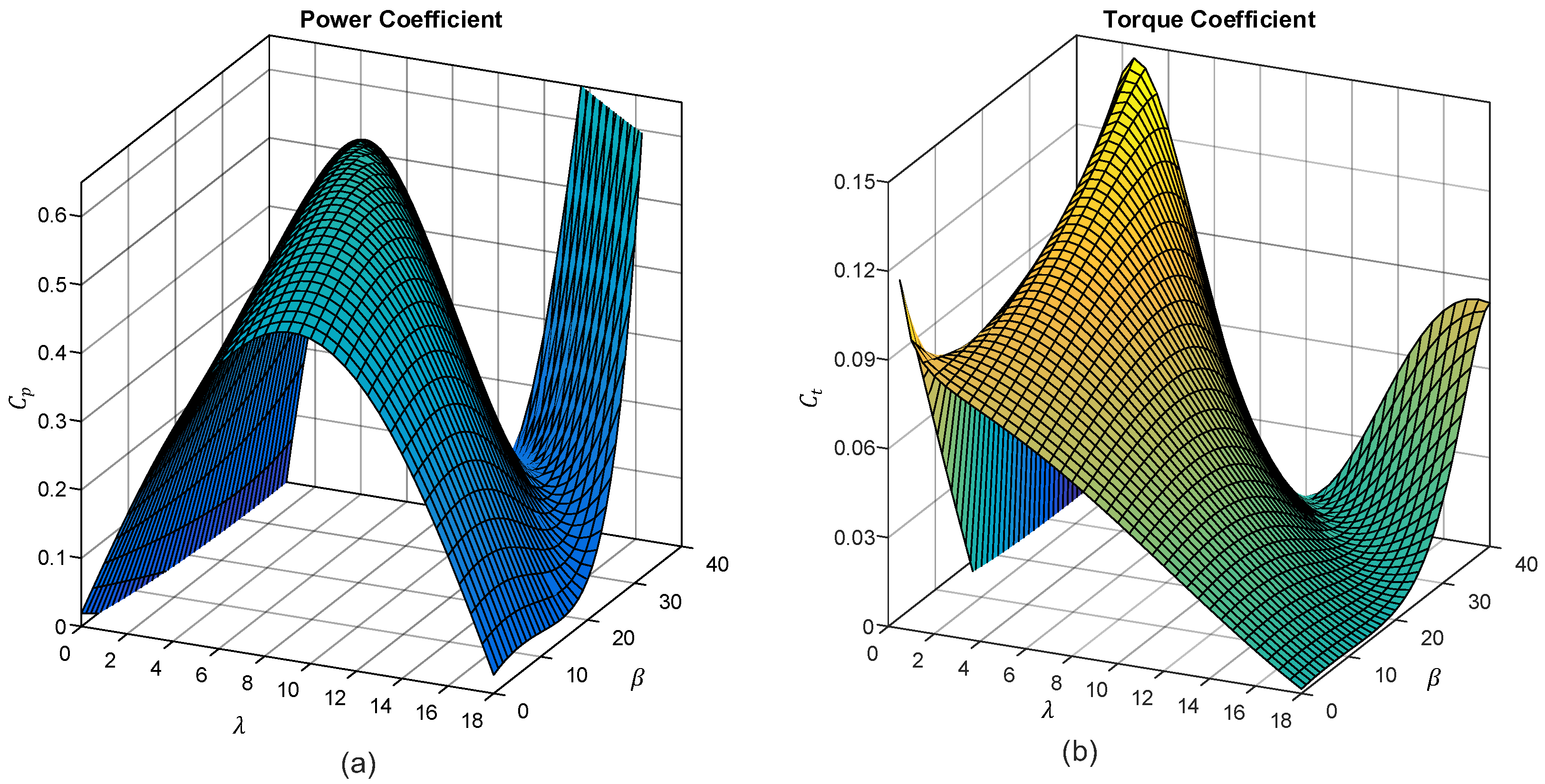
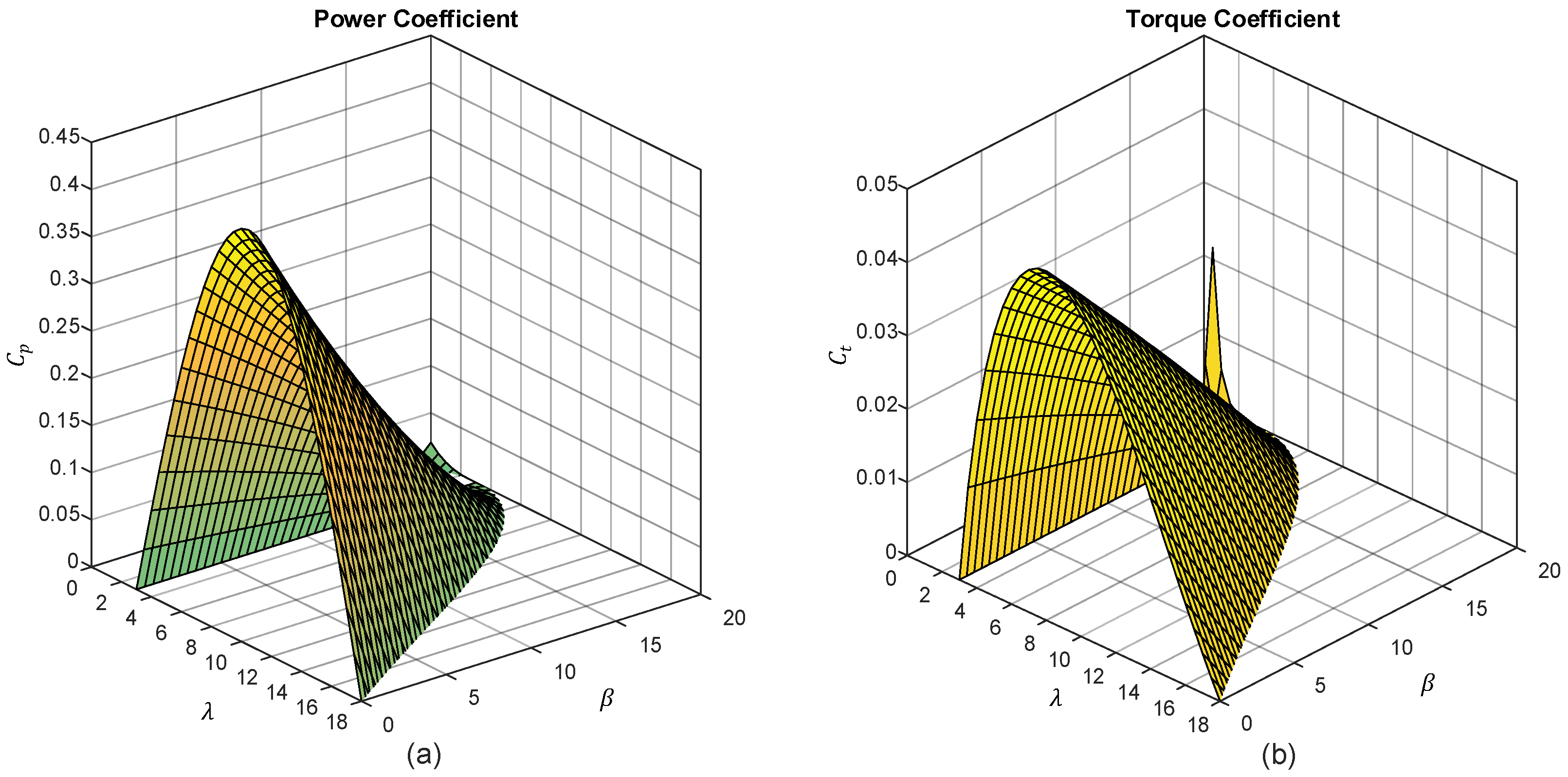
4.2. Discussion Considering Both Variations of λ and β

For the cases where variations in λ and β are analyzed, it is observed that the point where the value of the coefficients is higher occurs when β is equal to zero, except for the power coefficients proposed by Moussa, Bouallegue, and Kehedher [19] and Nouira and Khedher [13], which are based on a sinusoidal function, where the maximum value of $C_p$ is observed at other values different from β = 0. Additionally, the coefficient proposed by Moussa, Bouallegue, and Kehedher [19] has a problem for high values of both λ and β, because, once the value of $C_p$ decreases, it increases again, which does not happen with real wind turbines.

The coefficients based on a single sinusoidal function that presents an adequate behavior for both the $C_p$ and the $C_t$ is that proposed by Xin, Wanli, Bin, and Pengcheng [28], because, as the value of β increases, the values of $C_p$ and $C_t$ decrease; it is therefore suitable to apply a control based on β. For the coefficient proposed by Merahi, Mekhilef, and Madjid [29], the behavior of the power coefficient is adequate; however, the power coefficient tends to infinity through variations of λ and β.

In relation to the coefficients based on exponential functions, those that present real behaviors are those proposed by Kotti, Janakiraman, and Shireen [30], Khajuria and Kaur [32], Shi, Zhu, Cai, Wang, and Yao [49,50], and Ahmed, Karim, and Ahmad [42]. This is because they are the ones where the values of beta $C_p$ and $C_t$ increase, meaning that these systems can apply control techniques based on β. The remaining coefficients based on a sine function show the real behavior of $C_p$; however, the behavior of $C_t$ does not correspond to a real turbine, because the value of $C_t$ begins to decrease as β begins to increase, but, as β continues to increase, the value of $C_t$ also increases, which is not real and therefore cannot use control techniques based on β.

5. Conclusions

From the literature review carried out with the objective of analyzing the behavior of the power and torque coefficient proposed by different authors, it was found that they are expressed according to mathematical functions based on polynomial, sinusoidal, and exponential equations. These are obtained according to the physical characteristics of the turbines, such as the number of blades, construction materials, the shape of the blades, and β. Therefore, from the mathematical analysis, these coefficients can be seen to essentially depend on three mathematical functions based on each of them in a specific function (polynomial, sinusoidal, or exponential). In this paper, they were classified according to these functions; in the case of coefficients based on sinusoidal and exponential functions, a general equation was obtained. In relation to the general equations obtained, Table 2 and Table 3 were established; in these tables, the constants for each analyzed coefficient are established and grouped according to their mathematical model. The coefficients based on polynomial functions only depend on λ, and its operating range must be adequately limited in order to avoid generating non-real turbine behaviors. For example, for low values of the specific velocity, coefficient values are obtained of power that tends to infinity. The coefficients based on sinusoidal and exponential functions depend on λ and β; in this case, it is observed that the maximum value of the power coefficient is obtained when β is zero. In addition, it should be noted that, as β increases, the values of the power and torque coefficient must decrease in order to apply active control techniques of the turbines based on β. However, not all of the coefficients that have been proposed have this characteristic, so it is desirable that their behavior be adequately evaluated. This review offers an overview of all the power coefficients presented in the literature that serve to develop emulators of wind generation systems, develop and evaluate search algorithms of the maximum power point, and have active control techniques by varying β, among other applications.

References

1. Qadir, S.A.; Al-Motairi, H.; Tahir, F.; Al-Fagih, L. Incentives and strategies for financing the renewable energy transition: A review. Energy Rep. 2021, 7, 3590–3606. [Google Scholar] [CrossRef]
2. Liu, Y.; Dong, K.; Jiang, Q. Assessing energy vulnerability and its impact on carbon emissions: A global case. Energy Econ. 2023, 119, 106557. [Google Scholar] [CrossRef]
3. Al-Shetwi, A.Q. Sustainable development of renewable energy integrated power sector: Trends, environmental impacts, and recent challenges. Sci. Total Environ. 2022, 822, 153645. [Google Scholar] [CrossRef] [PubMed]
4. Androniceanu, A.; Sabie, O.M. Overview of Green Energy as a Real Strategic Option for Sustainable Development. Energies 2022, 15, 8573. [Google Scholar] [CrossRef]
5. Chudy-Laskowska, K.; Pisula, T. An Analysis of the Use of Energy from Conventional Fossil Fuels and Green Renewable Energy in the Context of the European Union’s Planned Energy Transformation. Energies 2022, 15, 7369. [Google Scholar] [CrossRef]
6. Arenas-López, J.P.; Badaoui, M. Analysis of the offshore wind resource and its economic assessment in two zones of Mexico. Sustain. Energy Technol. Assess. 2022, 52, 101997. [Google Scholar] [CrossRef]
7. Jung, C.; Schindler, D. Efficiency and effectiveness of global onshore wind energy utilization. Energy Convers. Manag. 2023, 280, 116788. [Google Scholar] [CrossRef]
8. Elgendi, M.; AlMallahi, M.; Abdelkhalig, A.; Selim, M.Y.E. A review of wind turbines in complex terrain. Int. J. Thermofluids 2023, 17, 100289. [Google Scholar] [CrossRef]
9. Li, M.; Yang, Y.; He, Z.; Guo, X.; Zhang, R.; Huang, B. A wind speed forecasting model based on multi-objective algorithm and interpretability learning. Energy 2023, 269, 126778. [Google Scholar] [CrossRef]
10. Arent, D.J.; Green, P.; Abdullah, Z.; Barnes, T.; Bauer, S.; Bernstein, A.; Berry, D.; Burrell, T.; Carpenter, B.; Cochran, J.; et al. Challenges and opportunities in decarbonizing the U.S. energy system. Renew. Sustain. Energy Rev. 2022, 169, 112939. [Google Scholar] [CrossRef]
11. Mayilsamy, G.; Palanimuthu, K.; Venkateswaran, R.; Antonysamy, R.P.; Lee, S.R.; Song, D.; Joo, Y.H. A Review of State Esti-mation Techniques for Grid-Connected PMSG-Based Wind Turbine Systems. Energies 2023, 16, 634. [Google Scholar] [CrossRef]
12. Rekioua, D. Wind Power Electric Systems; Springer: London, UK, 2014. [Google Scholar]
13. IEC 61400-12-1 Ed 1; Wind Turbines—Part 12-1: Power Performance, Measurements of Electricity Producing Wind Turbines. IEC: Geneva, Switzerland, 2005.
14. Xia, Y.; Ahmed, K.H.; Williams, B.W. Wind turbine power coefficient analysis of a new maximum power point tracking technique. IEEE Trans. Ind. Electron. 2013, 60, 1122–1132. [Google Scholar] [CrossRef]
15. Hwangbo, H.; Johnson, A.; Ding, Y. A production economics analysis for quantifying the efficiency of wind turbines. Wind Energy 2017, 20, 1501–1513. [Google Scholar] [CrossRef]
16. Niu, B.; Hwangbo, H.; Zeng, L.; Ding, Y. Evaluation of alternative power production efficiency metrics for offshore wind turbines and farms. Renew. Energy 2018, 128, 81–90. [Google Scholar] [CrossRef]
17. Lubosny, Z. Wind Turbine Operation in Electric Power Systems; Springer: Berlin/Heidelberg, Germany, 2003. [Google Scholar]
18. Nouira, I.; Khedher, A.; Bouallegue, A. A contribution to the design and the installation of an universal platform of a wind emulator using a DC motor. Int. J. Renew. Energy Res. 2012, 2, 797–804. [Google Scholar]
19. Moussa, I.; Bouallegue, A.; Khedher, A. Desing and Implementation of constant wind speed turbine emulator using Matlab/simulink and FPGA. In Proceedings of the 2014 Ninth International Conference on Ecological Vehicles and Renewable Energies (EVER), Monte-Carlo, Monaco, 25–27 March 2014. [Google Scholar]
20. Moussa, I.; Bouallegue, A.; Khedher, A. New wind turbine emulator based on DC machine: Hardware implementation using FPGA board for an open-loop operation. IET Circuits Devices Syst. 2019, 13, 896–9021. [Google Scholar] [CrossRef]
21. Arifujjaman, M.; Iqbal, M.; Quaicoe, J.E. Maximum Power Extraction from a Small Wind Turbine Emulator using a DC-DC Converter Controlled by a Microcontroller. In Proceedings of the 2006 International Conference on Electrical and Computer Engineering, Dhaka, Bangladesh, 19–21 December 2006; pp. 213–216. [Google Scholar]
22. Bhayo, M.A.; Yatim, A.H.M.; Khokhar, S.; Aziz, M.J.A.; Idris, N.R.N. Modeling of Wind Turbine Simulator for analysis of the wind energy conversion system using MATLAB/Simulink. In Proceedings of the 2015 IEEE Conference on Energy Conversion (CENCON), Johor Bahru, Malaysia, 19–20 October 2015; pp. 122–127. [Google Scholar]
23. González, L.G.; Figueres, E.; Garcera, G.; Carranza, O. Maximum-power-point tracking with reduced mechanical stress applied to wind-energy-conversion-systems. Appl. Energy 2010, 87, 2304–2312. [Google Scholar] [CrossRef] [Green Version]
24. Memije, D.; Rodríguez, J.J.; Carranza, O.; Ortega, R. Improving the performance of MPPT in a wind generation system using a wind speed estimation by Newton Raphson. In Proceedings of the IEEE International Autumn Meeting on Power, Electronics and Computing, ROPEC 2016, Ixtapa, Mexico, 9–11 November 2016. [Google Scholar]
25. Li, W.; Xu, D.; Zhang, W.; Ma, H. Research on Wind Turbine Emulation based on DC Motor. In Proceedings of the 2007 Second IEEE Conference on Industrial Electronics and Applications, Harbin, China, 23–25 May 2007. [Google Scholar]
26. Diaz, S.A.; Silva, C.; Juliet, J.; Miranda, H.A. Indirect sensorless speed control of a PMSG for wind application. In Proceedings of the 2009 IEEE International Electric Machines and Drives Conference, IEMDC ‘09, Miami, FL, USA, 3–6 May 2009; pp. 1844–1850. [Google Scholar]
27. Coto, J.; Garcia, M.; Diaz, G.; Gomez, J. Wind speed model design and dynamic simulation of a wind farm embedded on distribution networks. Renew. Energy Power Qual. J. 2003, 1, 341–348. [Google Scholar]
28. Xin, W.; Wanli, Z.; Bin, Q.; Pengcheng, L. Sliding mode control of pitch angle for direct driven PM Wind turbine. In Proceedings of the 26th Chinese Control and Decision Conference (2014 CCDC), Changsha, China, 31 May–2 June 2014; pp. 2447–2452. [Google Scholar]
29. Merahi, F.; Mekhilef, S.; Berkouk, E.M. DC-Voltage regulation of a five levels neutral point clamped cascaded for wind energy conversion system. In Proceedings of the 2014 International Power Electronics Conference, Hiroshima, Japan, 18–21 May 2014. [Google Scholar]
30. Kotti, R.; Janakiraman, S.; Shireen, W. Adaptive sensorless Maximum Power Point Tracking control for PMSG Wind Energy Conversion Systems. Paper P1-41. In Proceedings of the 2014 IEEE 15th Workshop on Control and Modeling for Power Electronics (COMPEL), Santander, Spain, 22–25 June 2014; pp. 1–8. [Google Scholar]
31. Barzola, J.; Simonetti, D.L.; Fardin, J.F. Energy storage systems for power oscillation damping in distributed generation based on wind turbines with PMSG. In Proceedings of the 2015 CHILEAN Conference on Electrical, Electronics Engineering, Information and Communication Technologies (CHILECON), Santiago, Chile, 28–30 October 2015; pp. 655–660. [Google Scholar]
32. Khajuria, S.; Kaur, J. Implementation of pitch control of wind turbine using Simulink (Matlab). Int. J. Adv. Res. Comput. Eng. Technol. 2012, 1, 196–200. [Google Scholar]
33. Ovando, R.I.; Aguayo, J.; Cotorogea, M. Emulation of a low power wind turbine with a DC motor in Matlab/Simulink. In Proceedings of the 2007 IEEE Power Electronics Specialists Conference, Orlando, FL, USA, 17–21 June 2007. [Google Scholar]
34. Cao, R.; Lu, L.; Xie, Z.; Zhang, X.; Yang, S. A dynamic wind turbine simulator of the wind turbine generator system. In Proceedings of the International Conference on Intelligent System Design and Engineering Application, Sanya, China, 6–7 January 2012. [Google Scholar]
35. Jin, Z.; Li, F.; Ma, X.; Djouadi, S.M. Semi-Definite Programming for Power Output Control in a Wind Energy Conversion System. IEEE Trans. Sustain. Energy 2014, 5, 466–475. [Google Scholar] [CrossRef]
36. Aree, P.; Lhaksup, S. Dynamic simulation of self-excited induction generator feeding motor load using Matlab/Simulink. In Proceedings of the 2014 11th International Conference on Electrical Engineering/Electronics, Computer, Telecommunications and Information Technology (ECTI-CON), Nakhon Ratchasima, Thailand, 14–17 May 2014; pp. 1–6. [Google Scholar]
37. Duman, S.; Yorukeren, N.; Altas, I.H.; Sharaf, A.M. A novel FACTS based on modulated power filter compensator for wind-grid energy systems. In Proceedings of the IEEE 5th International Symposium on Power Electronics for Distributed Generation Systems (PEDG), Galway, Ireland, 24–27 June 2014. [Google Scholar]
38. Cultura, A.B.; Salameh, Z.M. Modeling and simulation of a wind turbine-generator system. In Proceedings of the 2011 IEEE Power and Energy Society General Meeting, Detroit, MI, USA, 24–28 July 2011; pp. 1–7. [Google Scholar]
39. Guo, Y.; Hosseini, S.H.; Jiang, J.N.; Tang, C.Y.; Ramakumar, R.G. Voltage/Pitch control for maximization and regulation of active/reactive powers in wind turbines with uncertainties. In Proceedings of the 49th IEEE Conference on Decision and Control (CDC), Atlanta, GA, USA, 15–17 December 2010; pp. 3956–3963. [Google Scholar]
40. Hamane, B.; Doumbia, M.L.; Bouhamida, M.; Benghanem, M. Control of wind turbine based on DFIG using Fuzzy-PI and Sliding Mode controllers. In Proceedings of the 2014 Ninth International Conference on Ecological Vehicles and Renewable Energies (EVER), Monte-Carlo, Monaco, 25–27 May 2014; pp. 1–8. [Google Scholar]
41. Guo, Y.; Hosseini, S.H.; Tang, C.Y.; Jiang, J.N. An approximate model of wind turbine control systems for wind farm power control. In Proceedings of the 2011 IEEE Power and Energy Society General Meeting, Detroit, MI, USA, 24–28 July 2011; pp. 1–7. [Google Scholar]
42. Gao, F.; Xu, D.P.; Lv, Y.G. Hybrid automaton modeling and global control of wind turbine generator. In Proceedings of the Seventh International Conference on Machine Learning and Cybernetics, Kunming, China, 12–15 July 2008. [Google Scholar]
43. Bagh, S.; Samuel, P.; Sharma, R.; Banerjee, S. Emulation of static and dynamic characteristics of a Wind turbine using Matlab/Simulink. In Proceedings of the 2012 2nd International Conference on Power, Control and Embedded Systems, Allahabad, India, 17–19 December 2012; pp. 1–6. [Google Scholar]
44. Yin, M.; Li, G.; Zhou, M.; Zhao, C. Modeling of the wind turbine with a permanent magnet synchronous generator for integration. In Proceedings of the IEEE Power Engineering Society General Meeting, Tampa, FL, USA, 24–28 June 2007; pp. 1–6. [Google Scholar]
45. Shi, Q.; Wang, G.; Fu, L.; Yuan, L.; Huang, H. State-space averaging model of wind turbine with PMSG and its virtual inertia control. In Proceedings of the IECON 2013-39th Annual Conference of the IEEE Industrial Electronics Society, Vienna, Austria, 10–13 November 2013; pp. 1880–1886. [Google Scholar]
46. Chen, J.; Wu, H.; Sun, M.; Jiang, W.; Cai, L.; Guo, C. Modeling and simulation of directly driven wind turbine with permanent magnet synchronous generator. In Proceedings of the IEEE PES Innovative Smart Grid Technologies, Tianjin, China, 21–24 May 2012; pp. 1–5. [Google Scholar]
47. Chen, J.; Jiang, D. Study on modeling and simulation of non-grid-connected wind turbine. In Proceedings of the 2009 World Non-Grid-Connected Wind Power and Energy Conference, Nanjing, China, 24–26 September 2009; pp. 1–5. [Google Scholar]
48. Llano, D.; Tatlow, M.; McMahon, R. Control algorithms for permanent magnet generators evaluated on a wind turbine emulator test-ring. In Proceedings of the 7th IET International Conference on Power Electronics, Manchester, UK, 6–7 October 2014. [Google Scholar]
49. Shi, G.; Zhu, M.; Cai, X.; Wang, Z.; Yao, L. Generalized average model of DC wind turbine with consideration of electrome-chanical transients. In Proceedings of the IECON 2013—39th Annual Conference of the IEEE, Vienna, Austria, 10–13 November 2013. [Google Scholar]
50. Boukettaya, G.; Naifar, O.; Ouali, A. A vector control of a cascaded doubly fed induction generator for a wind energy conversion system. In Proceedings of the 2014 IEEE 11th International Multi-Conference on Systems, Signals & Devices (SSD14), Barcelona, Spain, 11–14 February 2014; pp. 1–7. [Google Scholar]
51. Bustos, G.; Vargas, L.S.; Milla, F.; Saez, D.; Zareipour, H.; Nunez, A. Comparison of fixed speed wind turbines models: A case study. In Proceedings of the IECON 2012—38th Annual Conference on IEEE Industrial Electronics Society, Montreal, QC, Canada, 25–28 October 2012; pp. 961–966. [Google Scholar]
52. Ahmed, D.; Karim, F.; Ahmad, A. Design and modeling of low-speed axial flux permanent magnet generator for wind based micro-generation systems. In Proceedings of the 2014 International Conference on Robotics and Emerging Allied Technologies in Engineering (iCREATE), Islamabad, Pakistan, 22–24 April 2014; pp. 51–57. [Google Scholar]
Figure 1. A power coefficient that depends on λ and the type of wind turbine [17].
Energies 16 02774 g001
Figure 2. A power coefficient for a specific type of turbine, with variations of λ and β [17].
Energies 16 02774 g002
Figure 3. Torque coefficient that depends on λ and the type of wind turbine [17].
Energies 16 02774 g003
Figure 4. Torque coefficient for a specific type of turbine, with variations of λ and β.
Energies 16 02774 g004
Figure 5. Coefficients based on a polynomial function; (a) power coefficient, (b) torque coefficient.
Energies 16 02774 g005
Figure 6. Coefficient based on a sinusoidal function; (a) power coefficient, (b) torque coefficient. Moussa [19], Coto [27], Xin [28], Merahi [29] and Nouira [18].
Energies 16 02774 g006
Figure 7. Coefficient proposed by Moussa, Bouallegue, and Kehedher [19], with variations of λ and β ; (a) power coefficient, (b) torque coefficient.
Energies 16 02774 g007
Figure 8. Coefficient proposed by Xin, Wanli, Bin, and Pengcheng [28], with variations of λ and β ; (a) power coefficient, (b) torque coefficient.
Energies 16 02774 g008
Figure 9. Coefficient proposed by Merahi, Mekhilef, and Madjid [29], with variations of λ and β ; (a) power coefficient, (b) torque coefficient.
Energies 16 02774 g009
Figure 10. Coefficient proposed by Nouira and Khedher [18], with variations of λ and β ; (a) power coefficient, (b) torque coefficient.
Energies 16 02774 g010
Figure 11. Coefficients based on an exponential function; (a) power coefficient, (b) torque coefficient. Kotti [30,31], Khajuria [32], Ov ando [33,34,35,36,37,38,39,40,41], Feng [42,43,44,45,46,47], Llano [48], Shi [19,50], Bustos [51], Ahmed [52].
Energies 16 02774 g011
Figure 12. Coefficient proposed by Kotti, Janakiraman, and Shireen [30], with variations of λ and β ; (a) power coefficient, (b) torque coefficient.
Energies 16 02774 g012
Figure 13. Coefficient proposed by Khajuria and Kaur [32], with variations of λ and β ; (a) power coefficient, (b) torque coefficient.
Energies 16 02774 g013
Figure 14. Coefficient proposed by Ovando, Aguayo, and Cotorogea [33,34,35,36,37,38,39,40,41], with variations of λ and β ; (a) power coefficient, (b) torque coefficient.
Energies 16 02774 g014
Figure 15. Coefficient proposed by Feng Gao, Da-Ping Xui, and Yue-Gang Lv [42,43,44,45,46,47], with variations of λ and β ; (a) power coefficient, (b) torque coefficient.
Energies 16 02774 g015
Figure 16. Coefficient proposed by Llano, Tatlow, and McMahon [48], with variations of λ and β ; (a) power coefficient, (b) torque coefficient.
Energies 16 02774 g016
Figure 17. Coefficient proposed by Shi, Zhu, Cai, Wang, and Yao [49,50], with variations of λ and β ; (a) power coefficient, (b) torque coefficient.
Energies 16 02774 g017
Figure 18. Coefficient proposed by Bustos, Vargas, Milla, Saez, Zareipour, and Nuñez [51], with variations of λ and β ; (a) power coefficient, (b) torque coefficient.
Energies 16 02774 g018
Figure 19. Coefficient proposed by Ahmed, Karim, and Ahmad [52], with variations of λ and β ; (a) power coefficient, (b) torque coefficient.
Energies 16 02774 g019