

Wind Turbine Blade Icing Prediction Using Focal Loss Function and CNN-Attention-GRU Algorithm


Abstract
1. Introduction
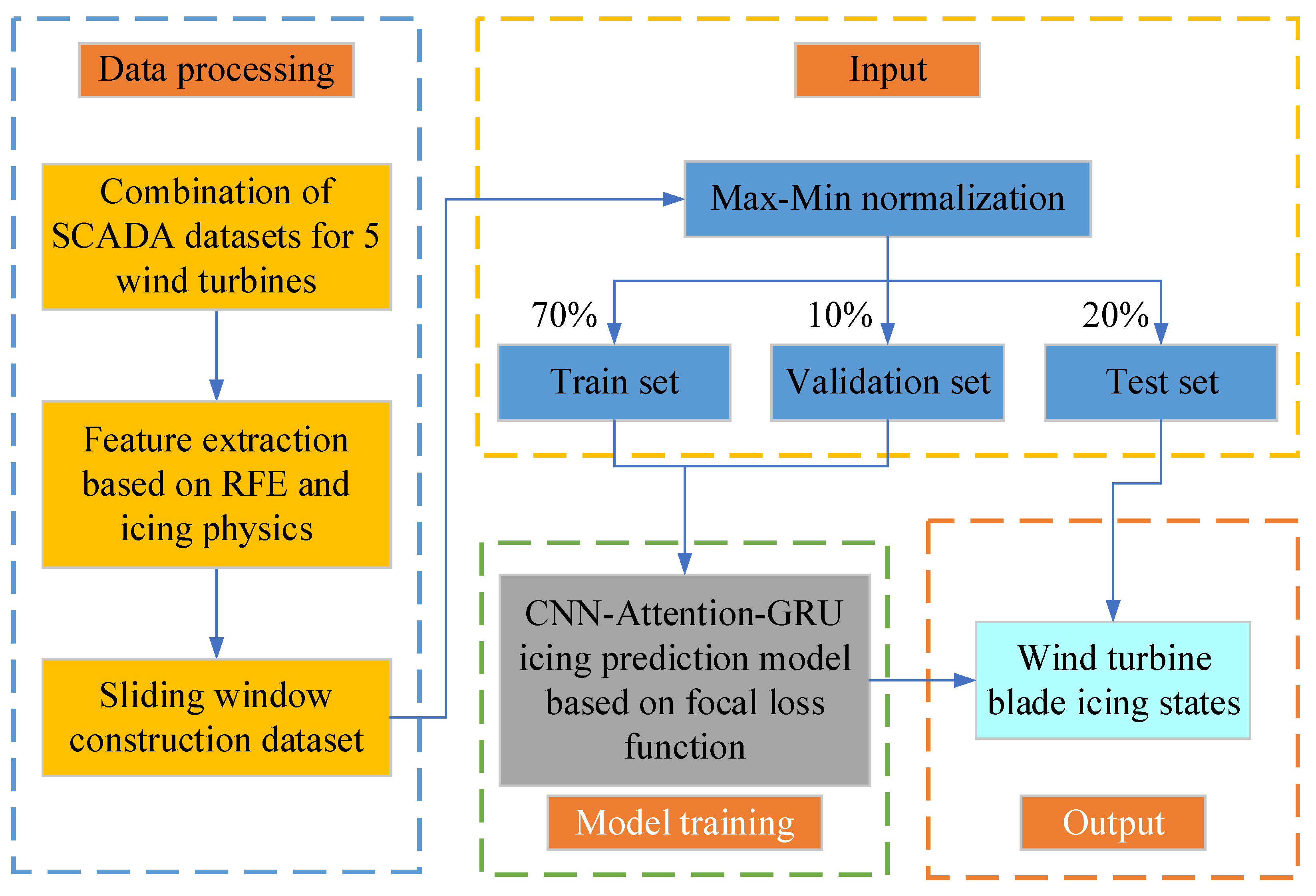
2. Data Processing
2.1. Feature Extraction
2.1.1. Recursive Feature Elimination
2.1.2. Feature Construction Based on Icing Physics
- (1)
- Theoretical power
- (2)
- Tip speed ratio
- (3)
- The square of wind speed
- (4)
- The cube of wind speed
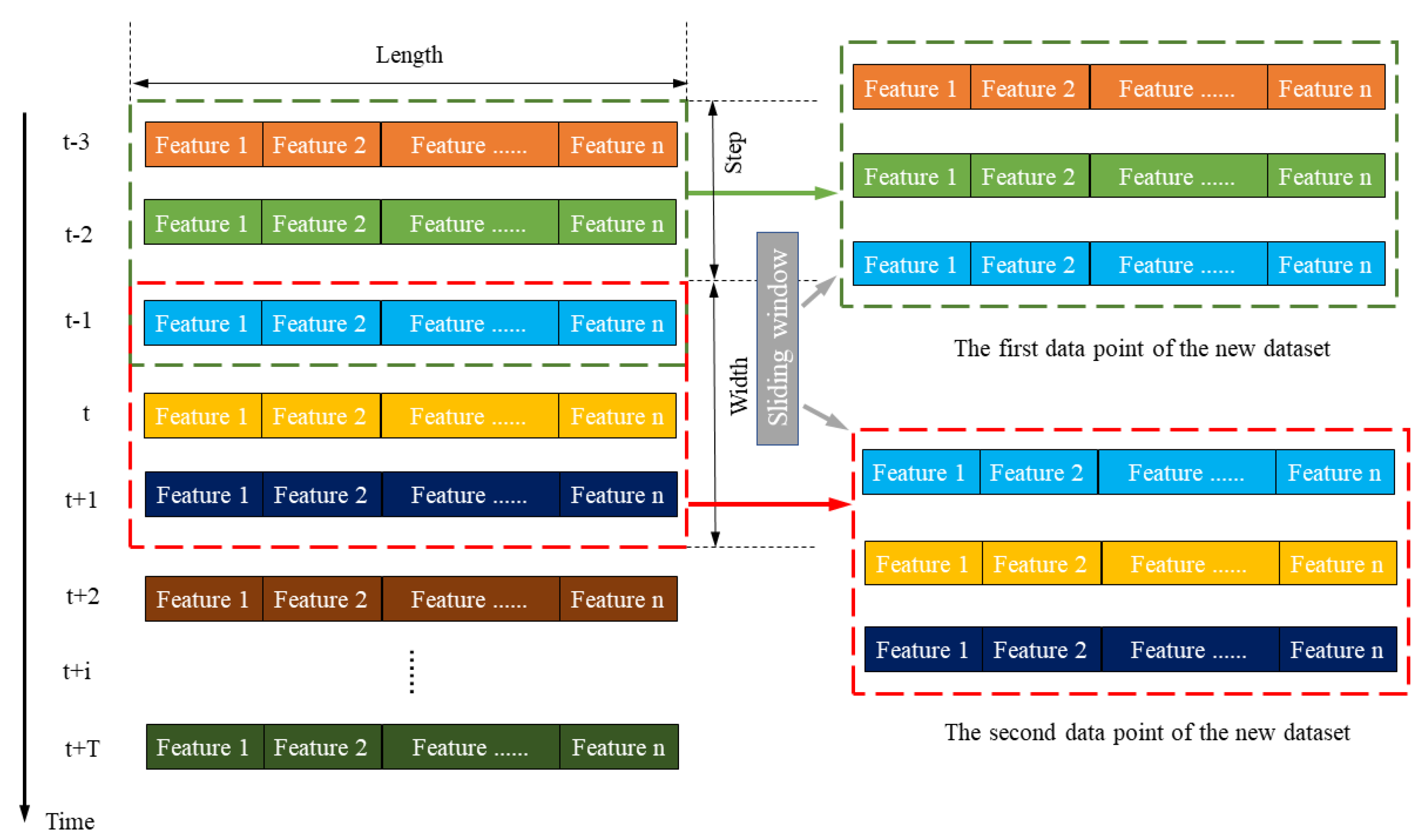
2.2. Constructing Dataset Based on Sliding Window Algorithm
2.3. Max–Min Normalization
3. Model Building
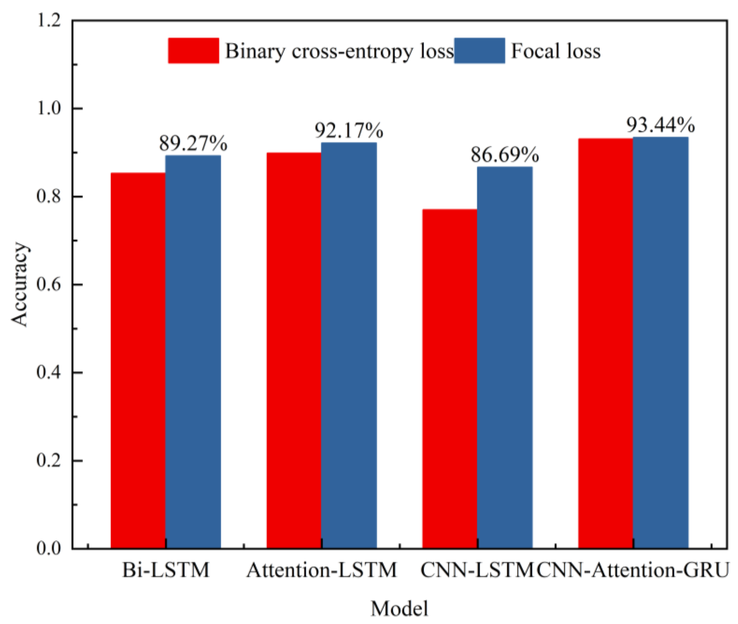
3.1. Focal Loss Function
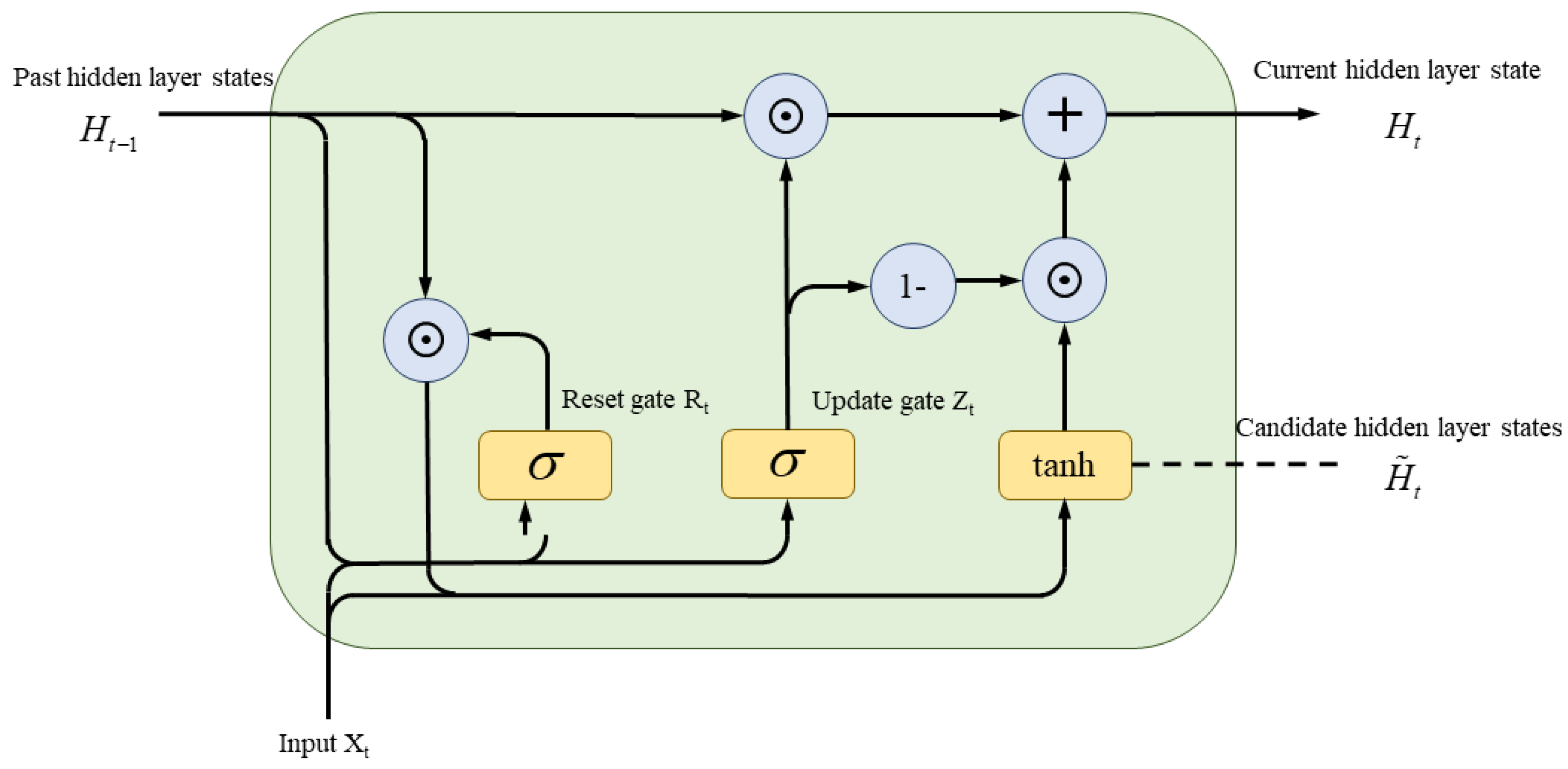
3.2. GRU Neural Network
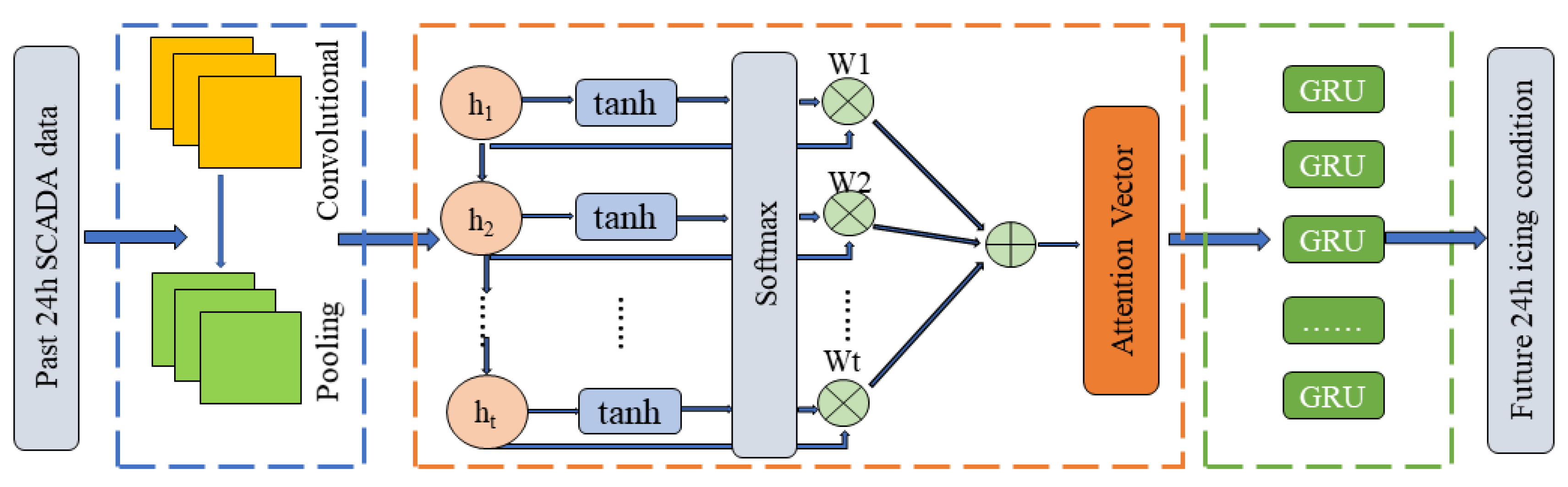
3.3. CNN Neural Network
3.4. Attention Mechanism
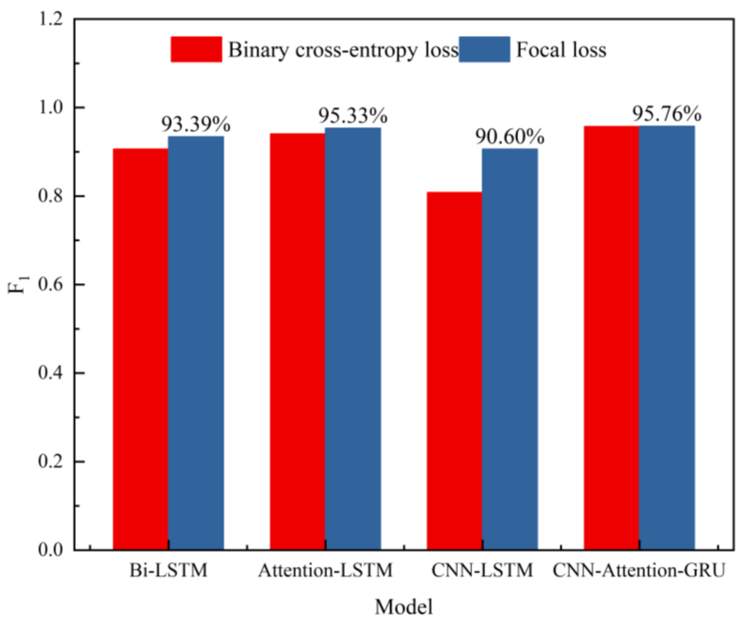
3.5. Evaluation Metrics
4. Case Study
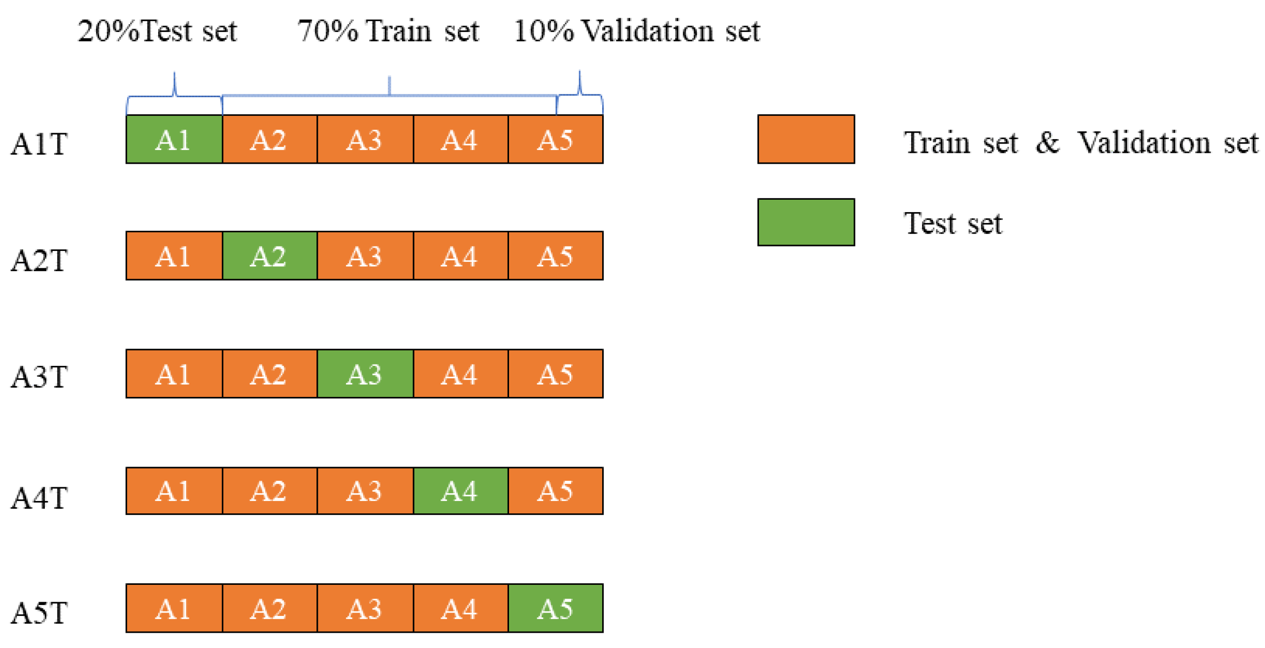
4.1. Data Description
4.2. Verification of the Validity of the Focal Loss Function
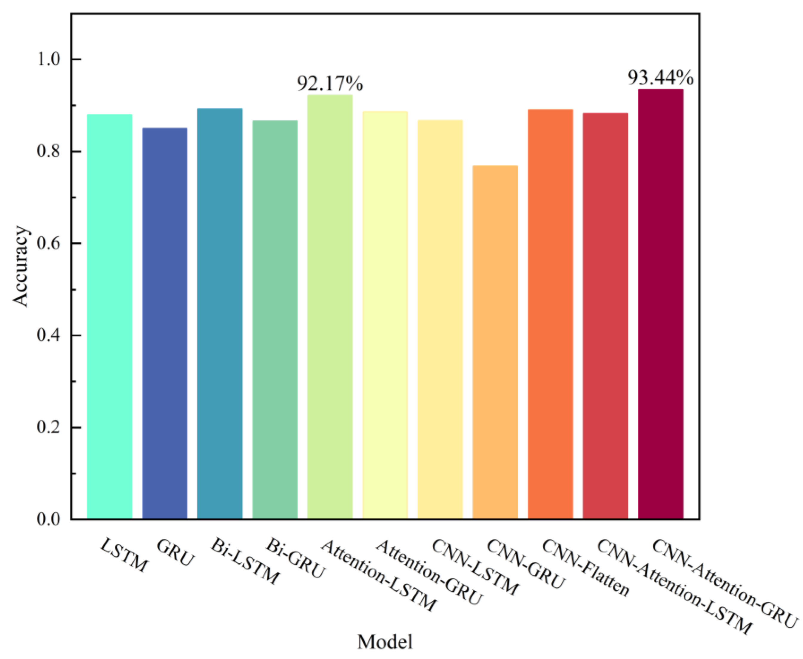
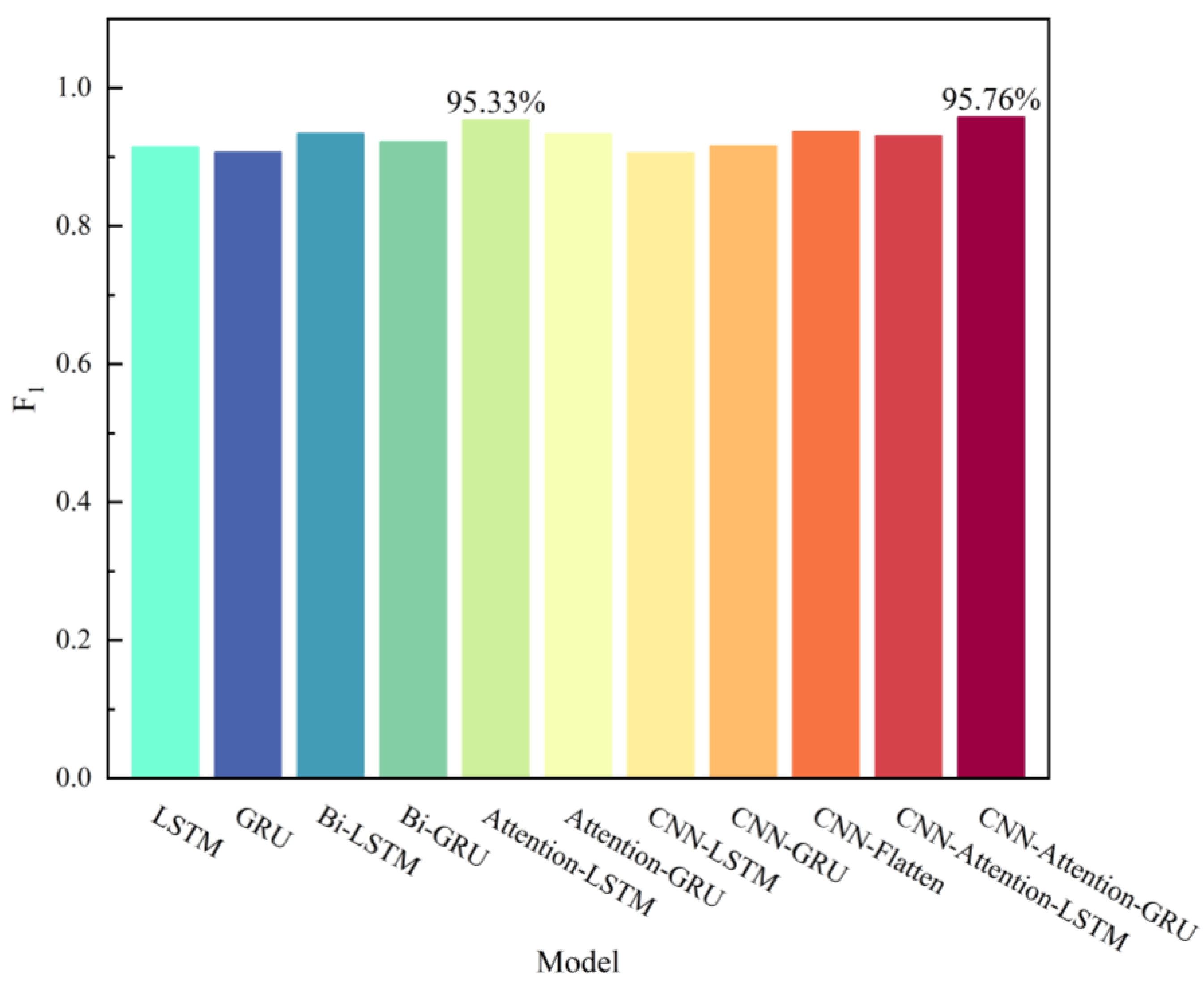
4.3. Prediction Accuracy Validation of the CNN-Attention-GRU Model
5. Conclusions
Author Contributions
Funding
Data Availability Statement
Conflicts of Interest
References
- Wang, W.; Qin, C.; Zhang, J.; Wen, C.; Xu, G. Correlation Analysis of Three-Parameter Weibull Distribution Parameters with Wind Energy Characteristics in a Semi-Urban Environment. Energy Rep. 2022, 8, 8480–8498. [Google Scholar] [CrossRef]
- Liu, H.; Li, Y.; Duan, Z.; Chen, C. A Review on Multi-Objective Optimization Framework in Wind Energy Forecasting Techniques and Applications. Energy Convers. Manag. 2020, 224, 113324. [Google Scholar] [CrossRef]
- Ibrahim, G.M.; Pope, K.; Naterer, G.F. Extended Scaling Approach for Droplet Flow and Glaze Ice Accretion on a Rotating Wind Turbine Blade. J. Wind Eng. Ind. Aerodyn. 2023, 233, 105296. [Google Scholar] [CrossRef]
- Dai, Y.; Xie, F.; Li, B.; Wang, C.; Shi, K. Effect of Blade Tips Ice on Vibration Performance of Wind Turbines. Energy Rep. 2023, 9, 622–629. [Google Scholar] [CrossRef]
- Hu, Q.; Xu, X.; Leng, D.; Shu, L.; Jiang, X.; Virk, M.; Yin, P. A Method for Measuring Ice Thickness of Wind Turbine Blades Based on Edge Detection. Cold Reg. Sci. Technol. 2021, 192, 103398. [Google Scholar] [CrossRef]
- Jin, J.Y.; Virk, M.S. Experimental Study of Ice Accretion on S826 & S832 Wind Turbine Blade Profiles. Cold Reg. Sci. Technol. 2020, 169, 102913. [Google Scholar] [CrossRef]
- Hacıefendioğlu, K.; Başağa, H.B.; Yavuz, Z.; Karimi, M.T. Intelligent Ice Detection on Wind Turbine Blades Using Semantic Segmentation and Class Activation Map Approaches Based on Deep Learning Method. Renew. Energy 2022, 182, 1–16. [Google Scholar] [CrossRef]
- Guk, E.; Son, C.; Rieman, L.; Kim, T. Experimental Study on Ice Intensity and Type Detection for Wind Turbine Blades with Multi-Channel Thermocouple Array Sensor. Cold Reg. Sci. Technol. 2021, 189, 103297. [Google Scholar] [CrossRef]
- Kreutz, M.; Alla, A.A.; Eisenstadt, A.; Freitag, M.; Thoben, K.-D. Ice Detection on Rotor Blades of Wind Turbines Using RGB Images and Convolutional Neural Networks. Procedia CIRP 2020, 93, 1292–1297. [Google Scholar] [CrossRef]
- Madi, E.; Pope, K.; Huang, W.; Iqbal, T. A Review of Integrating Ice Detection and Mitigation for Wind Turbine Blades. Renew. Sustain. Energy Rev. 2019, 103, 269–281. [Google Scholar] [CrossRef]
- Owusu, K.P.; Kuhn, D.C.S.; Bibeau, E.L. Capacitive Probe for Ice Detection and Accretion Rate Measurement: Proof of Concept. Renew. Energy 2013, 50, 196–205. [Google Scholar] [CrossRef]
- Gao, H.; Rose, J.L. Ice Detection and Classification on an Aircraft Wing with Ultrasonic Shear Horizontal Guided Waves. IEEE Trans. Ultrason. Ferroelectr. Freq. Control 2009, 56, 334–344. [Google Scholar] [CrossRef] [PubMed]
- Gómez Muñoz, C.Q.; García Márquez, F.P.; Sánchez Tomás, J.M. Ice Detection Using Thermal Infrared Radiometry on Wind Turbine Blades. Measurement 2016, 93, 157–163. [Google Scholar] [CrossRef]
- Rizk, P.; Al Saleh, N.; Younes, R.; Ilinca, A.; Khoder, J. Hyperspectral Imaging Applied for the Detection of Wind Turbine Blade Damage and Icing. Remote Sens. Appl. Soc. Environ. 2020, 18, 100291. [Google Scholar] [CrossRef]
- Gao, L.; Hong, J. Wind Turbine Performance in Natural Icing Environments: A Field Characterization. Cold Reg. Sci. Technol. 2021, 181, 103193. [Google Scholar] [CrossRef]
- Shu, L.; Li, H.; Hu, Q.; Jiang, X.; Qiu, G.; McClure, G.; Yang, H. Study of Ice Accretion Feature and Power Characteristics of Wind Turbines at Natural Icing Environment. Cold Reg. Sci. Technol. 2018, 147, 45–54. [Google Scholar] [CrossRef]
- Villalpando, F.; Reggio, M.; Ilinca, A. Prediction of Ice Accretion and Anti-Icing Heating Power on Wind Turbine Blades Using Standard Commercial Software. Energy 2016, 114, 1041–1052. [Google Scholar] [CrossRef]
- Kreutz, M.; Alla, A.A.; Lütjen, M.; Ohlendorf, J.-H.; Freitag, M.; Thoben, K.-D.; Zimnol, F.; Greulich, A. Ice Prediction for Wind Turbine Rotor Blades with Time Series Data and a Deep Learning Approach. Cold Reg. Sci. Technol. 2023, 206, 103741. [Google Scholar] [CrossRef]
- Xiao, J.; Li, C.; Liu, B.; Huang, J.; Xie, L. Prediction of Wind Turbine Blade Icing Fault Based on Selective Deep Ensemble Model. Knowl.-Based Syst. 2022, 242, 108290. [Google Scholar] [CrossRef]
- Cheng, P.; Jing, H.; Hao, C.; Xinpan, Y.; Xiaojun, D. Icing Prediction of Fan Blade Based on a Hybrid Model. Int. J. Perform. Eng. 2019, 15, 2882. [Google Scholar] [CrossRef]
- Ma, J.; Ma, L.; Tian, X. Wind Turbine Blade Icing Prediction Based on Deep Belief Network. In Proceedings of the 2019 4th International Conference on Mechanical, Control and Computer Engineering (ICMCCE), Hohhot, China, 24–26 October 2019; pp. 26–263. [Google Scholar]
- Bai, X.; Tao, T.; Gao, L.; Tao, C.; Liu, Y. Wind Turbine Blade Icing Diagnosis Using RFECV-TSVM Pseudo-Sample Processing. Renew. Energy 2023, 211, 412–419. [Google Scholar] [CrossRef]
- Tao, T.; Liu, Y.; Qiao, Y.; Gao, L.; Lu, J.; Zhang, C.; Wang, Y. Wind Turbine Blade Icing Diagnosis Using Hybrid Features and Stacked-XGBoost Algorithm. Renew. Energy 2021, 180, 1004–1013. [Google Scholar] [CrossRef]
- Li, F.; Cui, H.; Su, H.; Ma, Z.; Zhu, Y.; Zhang, Y. Icing Condition Prediction of Wind Turbine Blade by Using Artificial Neural Network Based on Modal Frequency. Cold Reg. Sci. Technol. 2022, 194, 103467. [Google Scholar] [CrossRef]
- Kreutz, M.; Alla, A.A.; Varasteh, K.; Ohlendorf, J.-H.; Lütjen, M.; Freitag, M.; Thoben, K.-D. Convolutional Neural Network with Dual Inputs for Time Series Ice Prediction on Rotor Blades of Wind Turbines. Procedia CIRP 2021, 104, 446–451. [Google Scholar] [CrossRef]
- Albashish, D.; Hammouri, A.I.; Braik, M.; Atwan, J.; Sahran, S. Binary Biogeography-Based Optimization Based SVM-RFE for Feature Selection. Appl. Soft Comput. 2021, 101, 107026. [Google Scholar] [CrossRef]
- Zeng, Z.; Cui, L.; Qian, M.; Zhang, Z.; Wei, K. A Survey on Sliding Window Sketch for Network Measurement. Comput. Netw. 2023, 226, 109696. [Google Scholar] [CrossRef]
- Cai, J.; Wang, S.; Xu, C.; Guo, W. Unsupervised Deep Clustering via Contractive Feature Representation and Focal Loss. Pattern Recognit. 2022, 123, 108386. [Google Scholar] [CrossRef]
- Chen, J.; Fu, C.; Xie, H.; Zheng, X.; Geng, R.; Sham, C.-W. Uncertainty Teacher with Dense Focal Loss for Semi-Supervised Medical Image Segmentation. Comput. Biol. Med. 2022, 149, 106034. [Google Scholar] [CrossRef]
- Wu, Y.; Ma, X. A Hybrid LSTM-KLD Approach to Condition Monitoring of Operational Wind Turbines. Renew. Energy 2022, 181, 554–566. [Google Scholar] [CrossRef]
- Cao, L.; Zhang, H.; Meng, Z.; Wang, X. A Parallel GRU with Dual-Stage Attention Mechanism Model Integrating Uncertainty Quantification for Probabilistic RUL Prediction of Wind Turbine Bearings. Reliab. Eng. Syst. Saf. 2023, 235, 109197. [Google Scholar] [CrossRef]
- Abbaskhah, A.; Sedighi, H.; Akbarzadeh, P.; Salavatipour, A. Optimization of Horizontal Axis Wind Turbine Performance with the Dimpled Blades by Using CNN and MLP Models. Ocean Eng. 2023, 276, 114185. [Google Scholar] [CrossRef]
- Jiang, G.; Yue, R.; He, Q.; Xie, P.; Li, X. Imbalanced Learning for Wind Turbine Blade Icing Detection via Spatio-Temporal Attention Model with a Self-Adaptive Weight Loss Function. Expert Syst. Appl. 2023, 229, 120428. [Google Scholar] [CrossRef]


| Feature Names | |
|---|---|
| Actual power | Gear oil temperature |
| Wind speed | Gearbox bearing temperature |
| Generator speed | Generator temperature |
| Ambient temperature | Theoretical power |
| Nacelle temperature | Tip speed ratio |
| Yaw angle | The square of wind speed |
| Wind direction | The cube of wind speed |
| Feature Name | Feature Description | Feature Name | Feature Description |
|---|---|---|---|
| WIND_SPEED | Wind speed | GENGNTMP | Generator temperature |
| REAL_POWER | The active power of grid-side | GENAPHSA | Current of A-phase |
| CONVERTER_MOTOR_SPEED | Generator speed | GENAPHSB | Current of B-phase |
| ROTOR_SPEED | Blade rotation speed | GENAPHSC | Current of C-phase |
| WIND_DIRECTION | Wind direction | GENVPHSA | Voltage of A-phase |
| TURYAWDIR | Yaw angle | GENVPHSB | Voltage of B-phase |
| GBXOILTMP | Temperature of gear oil | GENVPHSC | Voltage of C-phase |
| GBXSHFTMP | Temperature of gearbox bearing | GENHZ | Frequency of motor |
| EXLTMP | Temperature of environment | TURPWRREACT | Reactive power |
| TURINTTMP | Temperature of nacelle |
| Wind Turbine Number | Total Number of Data | Normal Data | Icing Data |
|---|---|---|---|
| A1 | 1009 | 857 (84.94%) | 152 (15.06%) |
| A2 | 1009 | 857 (84.94%) | 152 (15.06%) |
| A3 | 997 | 831 (83.35%) | 167 (16.65%) |
| A4 | 1009 | 849 (84.14%) | 160 (15.86%) |
| A5 | 1009 | 826 (81.86%) | 183 (18.14%) |
| Model | Accuracy | F1 | ||||||||||
|---|---|---|---|---|---|---|---|---|---|---|---|---|
| A1T | A2T | A3T | A4T | A5T | Average | A1T | A2T | A3T | A4T | A5T | Average | |
| LSTM | 0.9222 | 0.9597 | 0.8787 | 0.9694 | 0.6667 | 0.8793 | 0.9482 | 0.9739 | 0.9266 | 0.9808 | 0.7425 | 0.9144 |
| GRU | 0.9083 | 0.7222 | 0.8082 | 0.9708 | 0.8403 | 0.8500 | 0.9384 | 0.8279 | 0.8887 | 0.9816 | 0.898 | 0.9069 |
| Bi-LSTM | 0.9653 | 0.7806 | 0.9859 | 0.9847 | 0.7472 | 0.8927 | 0.9775 | 0.8556 | 0.9909 | 0.9903 | 0.8553 | 0.9339 |
| Bi-GRU | 0.975 | 0.8458 | 0.7884 | 0.9736 | 0.7472 | 0.8660 | 0.9839 | 0.9095 | 0.8786 | 0.9833 | 0.8553 | 0.9221 |
| Attention-LSTM | 0.9708 | 0.9403 | 0.9972 | 0.9333 | 0.7667 | 0.9217 | 0.9814 | 0.9628 | 0.9982 | 0.959 | 0.865 | 0.9533 |
| Attention-GRU | 0.9819 | 0.8444 | 0.9986 | 0.8556 | 0.7472 | 0.8855 | 0.9884 | 0.9079 | 0.9991 | 0.9152 | 0.8553 | 0.9332 |
| CNN-LSTM | 0.7597 | 0.9389 | 0.976 | 0.9153 | 0.7444 | 0.8669 | 0.8207 | 0.9613 | 0.9846 | 0.9484 | 0.8149 | 0.9060 |
| CNN-GRU | 0.6014 | 0.7722 | 0.8999 | 0.9597 | 0.6069 | 0.7680 | 0.6627 | 0.8316 | 0.9386 | 0.9748 | 0.6705 | 0.8156 |
| CNN-Flatten | 0.9403 | 0.8181 | 0.969 | 0.9625 | 0.7639 | 0.8908 | 0.9609 | 0.8868 | 0.9801 | 0.9765 | 0.8636 | 0.9336 |
| CNN-Attention-LSTM | 0.9764 | 0.9028 | 0.9492 | 0.8361 | 0.7472 | 0.8823 | 0.9848 | 0.9383 | 0.9679 | 0.9048 | 0.8553 | 0.9302 |
| CNN-Attention-GRU | 0.9153 | 0.9278 | 0.9803 | 0.9069 | 0.9417 | 0.9344 | 0.9434 | 0.9521 | 0.9873 | 0.9437 | 0.9615 | 0.9576 |
Disclaimer/Publisher’s Note: The statements, opinions and data contained in all publications are solely those of the individual author(s) and contributor(s) and not of MDPI and/or the editor(s). MDPI and/or the editor(s) disclaim responsibility for any injury to people or property resulting from any ideas, methods, instructions or products referred to in the content. |
© 2023 by the authors. Licensee MDPI, Basel, Switzerland. This article is an open access article distributed under the terms and conditions of the Creative Commons Attribution (CC BY) license (https://creativecommons.org/licenses/by/4.0/).
Share and Cite
Tao, C.; Tao, T.; Bai, X.; Liu, Y. Wind Turbine Blade Icing Prediction Using Focal Loss Function and CNN-Attention-GRU Algorithm. Energies 2023, 16, 5621. https://doi.org/10.3390/en16155621
Tao C, Tao T, Bai X, Liu Y. Wind Turbine Blade Icing Prediction Using Focal Loss Function and CNN-Attention-GRU Algorithm. Energies. 2023; 16(15):5621. https://doi.org/10.3390/en16155621
Chicago/Turabian StyleTao, Cheng, Tao Tao, Xinjian Bai, and Yongqian Liu. 2023. "Wind Turbine Blade Icing Prediction Using Focal Loss Function and CNN-Attention-GRU Algorithm" Energies 16, no. 15: 5621. https://doi.org/10.3390/en16155621
APA StyleTao, C., Tao, T., Bai, X., & Liu, Y. (2023). Wind Turbine Blade Icing Prediction Using Focal Loss Function and CNN-Attention-GRU Algorithm. Energies, 16(15), 5621. https://doi.org/10.3390/en16155621