Abstract
The annual target reliability level for structural components is given as β = 3.3 in the main design standard for wind turbines IEC 61400-1 ed. 4. However, since the same safety factors are used for a range of load cases and limit states, deviations in the obtained reliability level can be expected, and it should be considered how to handle this in relation to the development of the IEC TS 61400-9 on probabilistic design measures. In this paper, structural reliability analyses were performed for components designed using safety factors for a range of extreme load cases, and by using the correlation between limit states for different years, the development of the reliability level over time was calculated. A relative risk-based assessment was applied to assess the optimal target reliability level and safety factors. The risk-based assessment explicitly includes the uncertainties, benefits, and costs and can motivate differentiation of the annual reliability level between load cases. Annual reliability indices were found to be in the range of 2.9–3.4, and although this includes values below the target of 3.3, it was also found that the optimal reliability indices were in the same range. The variation in reliability level can be motivated since the optimal target reliability is found to be lower than the current target for load cases with high correlation, as this causes the lifetime reliability level to be comparable to that of other extreme load cases with less correlation.
1. Introduction
The drive for cost reductions within wind energy motivates the search for ways to achieve optimized and less conservative wind turbine designs while still fulfilling basic reliability requirements. For some optimization tasks (e.g., regarding the blades [1] and wind farm layout [2]), both the power production and material usage need to be considered, whereas for structural optimization of the jacket topology [3] or monopile cross-section [4], the production is not affected. Ideally, a holistic perspective should be applied, where expenses for design, manufacturing, transport, installation, and maintenance are included. However, regarding the structural design of components, optimization typically implies finding the smallest design parameter, i.e., cross-section, which fulfills the design criteria.
Currently, a deterministic design procedure is generally applied, where load cases and safety factors from the main design standard IEC 61400-1 [5] are used. One of the possible ways to achieve cost reductions is through the use of probabilistic design methods, where data from tests, measurement campaigns, and operational experience can be used to reduce uncertainties, thus allowing for a less conservative design [6]. Previous research has examined the relationship between safety factors and reliability level concerning fatigue of welded and cast steel details [7], fatigue reliability of large monopiles [8], fatigue reliability for concrete sub-structures [9], and extreme load effects from combined wind and wave loading on offshore wind turbines in [10] and extended to large monopiles in [11]. Further, reliability analyses may be applied in relation to the integrity management of wind turbines, e.g., by performing reliability updating for structures using a digital twin [12] or in relation to risk-based blade O&M [13]. Some studies suggest using surrogates as part of a reliability-based design procedure to increase computational efficiency [14] and perform efficient uncertainty propagation [15].
For the reliability-based design of wind turbines, a target reliability level should first be defined. For wind turbines, lower reliability levels are accepted compared to many other civil engineering structures, such as buildings, bridges, and oil and gas facilities, because the failure of a wind turbine does not lead to a large probability of fatalities or human injuries, it does not pose a large environmental threat, and it does not pose large consequences to the society. For the design of wind turbines, the main risk is, therefore, the economic loss due to the loss of power production. This means that the reliability level can be determined mainly based on economic risk-based considerations [16].
Until edition 4 of the main design standard for wind turbines IEC 61400-1 [5] was published in 2019, the reliability requirements were given only indirectly through the safety factors [17]. During the development of ed. 4 of IEC 61400-1 [5], a reliability background was developed to motivate the safety factors [17]. An annual reliability index was selected as the target for component class 2 based on ISO 2394 [18], and for selected design load cases (DLCs), safety factors were calibrated such that the target reliability level would be reached. However, the same partial safety factors are applied for a wider range of load cases, components, and environmental conditions, and this will typically result in variation in the obtained reliability level [19]. This implies that for some DLCs, the reliability level implicitly given through the safety factors is lower than the target , and in these cases, a reliability-based design will often lead to a more expensive design than a design based on safety factors [20]. Due to the demand for cheaper wind turbines, in practice, the cheaper design based on safety factors will be used. However, another option is to accept the lower reliability level implicitly given through the safety factors also for reliability-based design, thus allowing further optimization of the design if uncertainties can be reduced [21]. The lower reliability level should not be accepted by default but only if it can be justified based on a risk-based optimization that is more detailed than the model behind the original background for [22].
In the background document for the safety factors in IEC 61400-1 [17], the target is motivated mainly by the table of annual reliability indices in ISO 2394 [18] and JCSS Probabilistic Model Code [23], where the reliability target depends on the relative consequence of failure and the relative costs of increasing the reliability. In the background document, it is noted that the relative cost of increasing reliability is large because the cost of energy is important and that the consequences of failure are only economic. Further, it is noted that wind turbines are designed to the IEC wind turbine classes, thus not all wind turbines are designed to the limit. The table in [18,23] was originally developed by Rackwitz [22] and was elaborated by Fischer et al. [24]. The underlying assumption is that the failure rate and obsolescence rate are constant over time, and in case of failure or obsolescence, new structures are systematically constructed. This means that a risk-based optimization can be made using an infinite time horizon, and the benefits can be disregarded. According to this model, higher costs of increasing reliability lead to lower optimal target reliabilities, and higher failure costs lead to higher optimal reliabilities. If the uncertainties are larger, it leads to lower optimal reliability, as it will be more expensive to increase the reliability.
The assumption of a constant failure rate is not always accurate. An obvious example is the fatigue limit state, where the annual reliability index decreases with time. Although the current practice is to compare the annual failure probability in the worst year with the target value, this is a conservative approach. Rackwitz [22] originally noted that for fatigue, the target should be compared to the asymptotic value of the renewal density, which for a deterministic lifetime approximately corresponds to using the average annual failure probability. For fatigue, this will allow the failure probability to be larger than the target in the worst year.
Additionally, for extreme loading, the limit states for different years may be correlated due to shared resistance and model uncertainties, and thus the annual failure probability will not be constant over time. A correlation will mean that the annual failure probability decreases over time; thus, the failure probability will be the largest in the first year. Especially for load cases where the uncertainty on the annual maximum load is small (e.g., during normal operation), this effect can be significant.
In addition to the assumption of a constant failure rate, the assumption of systematic reconstruction is also not accurate for wind turbines. Wind turbines are today mostly erected in wind farms, and if one turbine in a wind farm fails, it is not likely that it will be replaced due to the high costs of installing just one wind turbine. Therefore, it becomes relevant to use a model with a finite time horizon, where benefits are included and where the failure rate is modeled more accurately. A finite horizon risk-based optimization model was developed for the assessment of the target reliability level for life extension [21] and life extension decision-making [25]. In these applications, the focus was the fatigue limit state, where it was utilized that the annual failure probability increases with time, i.e., if a turbine is designed to the limit, the annual failure probability is lower than the target in all other years than the last year.
In this work, the finite horizon risk-based optimization model is adapted for use in extreme design situations. We propose to utilize the correlation between limit states for different years in a relative comparison between load cases, to make a risk-based assessment of the reliability level and safety factors in IEC 61400-1. We limit the scope to extreme load cases without faults. The aim is to investigate whether the target reliability index (as stated in informative annex K of IEC 61400-1) is fulfilled for typical generic limit state equations and assess whether eventual differences in the reliability level can be motivated based on a risk-based assessment. This could be utilized for the reliability-based design of wind turbines in the coming IEC TS 61400-9 “Probabilistic design measures for wind turbines” [26] and would enable cost reductions while rationally considering the reliability. This paper presents work made by members of the project team for IEC TS 61400-9 [26] during the development of the technical specification. The main novelty is the procedure for the calculation of the variation in reliability over time for extreme limit states and the application of the risk-based models for the assessment of the optimal reliability level for extreme limit states.
The paper is structured as follows: Section 2 presents the methods used for reliability analysis, calculation of the reliability over time, and the risk-based assessment model. Section 3 presents and discusses the results of the reliability and risk-based assessment. Section 4 concludes the work with a broader discussion.
2. Methods
This section describes the methods and models used for estimating the annual reliability index and for estimating the optimal reliability level. An overview is given in Figure 1. The left side of the figure outlines the procedure used for estimating the reliability level in IEC61400-1. First, the design equation was used together with the safety factors to calculate the design parameter z. The reliability index was then calculated using Monte Carlo simulations based on a generic limit state equation. In both the design equation and limit state equation, normalized distributions were used for the resistance and load effect. This generic approach is typically applied for calibration of safety factors, as it eliminates the need for detailed design considerations, but it cannot be used for design, only for relative assessment where the normalized distributions provide the link between the design equation and the limit state equation [17]. The reliability indices calculated here were annual reliability indices in the first year of operation. Often, this is simply referred to as the annual reliability index with no mention of time, and this is sufficient to evaluate the maximum annual failure probability.
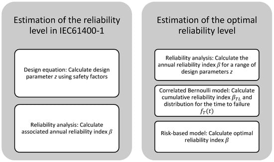
Figure 1.
Overview of the method. The design equation is described in Section 2.1, the reliability analysis in Section 2.2, the correlated Bernoulli model in Section 2.3, and the risk-based model in Section 2.4.
The right side of Figure 1 outlines the procedure for the estimation of the optimal reliability level. Here, a range of design parameters were first defined, and the annual reliability index was calculated for each value. Further, the correlation coefficient between limit states for different years was estimated. Based on the annual reliability index and the correlation coefficient, a correlated Bernoulli model was used to calculate the distribution for the time to failure. Finally, to estimate the optimal reliability level, the distribution for the time to failure was combined with a risk-based model.
This study focuses on load cases with extreme loading, and the following DLCs are considered:
- DLC 1.1: Extreme loads during power production (load extrapolation);
- DLC 1.3: Extreme loads during power production (extreme turbulence);
- DLC 6.1: Extreme wind speed during parked conditions (storm);
- DLC 6.1T: Extreme wind speed during parked conditions (typhoon);
- Gravity loading only.
The load case with only gravity loading is relevant because, according to IEC61400-1, the safety factor can be reduced for the other load cases, depending on the relative contribution of the gravity load to the characteristic load. The case with only gravity loading can be seen as the limit case.
2.1. Design Equation
The design equation for extreme loading is given as follows:
where z is the design parameter (e.g., a cross-sectional parameter); is the characteristic value of the resistance; is the characteristic value of the load effect; and , , and are safety factors. The safety factor for the resistance is when a 5% quantile is used as the characteristic value. The safety factor for the consequence of failure depends on the component class and is , , and for component classes 1, 2, and 3, respectively. Here, component class 2 is considered, as most structural elements belong to this class. The safety factor for the load effect is for normal design situations. An exception is DLC 1.1 when load extrapolation is used where . When there is only gravity loading, the safety factor for the load effect is . The characteristic value of the load effect is 98% quantile in the distribution for the annual maximum load, except for gravity loading, where the characteristic value is the mean value. For the typhoon class in IEC 61400-1, the design can be performed using the load safety factor for normal design situations. However, it is mentioned in a footnote that this safety factor is derived assuming that the coefficient of variation (COV) of the annual maximum wind speed is less than 15% and that the safety factor can be increased linearly by a factor from 1.0 at COV = 15% to 1.15 at COV = 30% [5] (p. 76). For a Typhoon wind with COV = 25% on the annual maximum wind speed, the factors are and . However, increasing the safety factor is not given as a requirement, and the design may be based on the normal safety factor .
The design equation can be used to find the necessary design parameter z for given values of the characteristic resistance and load effect .
2.2. Reliability Analysis
A reliability analysis was performed to calculate the annual reliability index obtained for a given value of the design parameter z. The reliability index is defined as , and where the annual probability of failure is calculated from the limit state equation as . The limit state equation is formulated as follows:
where z is the design parameter, models the resistance including uncertainties on the dominating strength parameter, models the load effect including physical uncertainties, is the model uncertainty on the resistance model, is the model uncertainty in the stress/strain model, is the uncertainty related to the site/atmospheric conditions, is the uncertainty in the aerodynamic properties, is the model uncertainty related to the structural dynamics, is the uncertainty due to variations in material and geometrical properties, is the model uncertainty in the wind model, and is the statistical uncertainty associated with the design process of sampling wind conditions with a limited number of simulations. The stochastic model for the load and resistance variables is shown in Table 1 and Table 2. For the Typhoon case, a COV = 50% is assumed on the load effect, which approximately corresponds to a COV = 25% on the wind speed, as the wind pressure is proportional to the squared wind speed. There is no common agreement on whether it is more appropriate to model the wind pressure or wind speed by a Gumbel distribution, and here the wind pressure is modeled by a Gumbel distribution [27]. The stochastic model is based on IEC CD TS 61400-9 [26].

Table 1.
Stochastic model for the load variables. Abbreviations are used for the distributions: LN: Lognormal, G: Gumbel, N: Normal.
Table 2.
Stochastic model for the resistance variables. LN: Lognormal distribution.
When the limit state equation and stochastic model are fully defined, the annual reliability index can be estimated using structural reliability methods such as the first-order reliability method (FORM), second-order reliability method (SORM), or simulation-based methods. In this study, crude Monte Carlo simulations were used. A highly efficient implementation based on elementwise computations was used where simulations can be performed in ~2 s on a standard laptop. Compared to a traditional implementation with loops, the computation time is reduced by a factor of ~500. In the simulation procedure, a -matrix is generated with standard normal distributed numbers (u-values), where is the number of stochastic variables in the limit state equation. Each column is transformed from the u-space to the x-space using the Rosenblatt transformation for the specific distribution, and the limit state equation is evaluated for each row.
To estimate the -vector, which indicates the importance of the different variables, first, the design point is estimated as the mean value of each column of the matrix with u-values, including only rows for the failed realizations, i.e., . This generally slightly overestimates the length of the -vector, as this point is located within the failure domain. However, for the estimation of the -vector, this is not important, as the -vector is obtained by normalizing the -vector.
2.3. Reliability over Time
When the reliability index is calculated using a limit state equation with a distribution for the maximum annual load, the calculated reliability index is an annual reliability index. If the aim is to calculate the expected number of failures over the lifetime of a fleet of wind turbines, the lifetime reliability index can be calculated.
If failures occur with a constant rate (a Poisson process), the time-to-failure distribution would be given by the exponential distribution, which decreases with time. When time is discretized, this will be a Bernoulli process, and the time-to-failure distribution is a geometric distribution. The probability that the first failure happens in the second year is slightly smaller than for the first year because the first failure cannot happen in the second year if it already failed in the first year. For the present stochastic model, the failure events are dependent due to time-invariant stochastic variables, i.e., model uncertainties and resistances. This gives a further decrease in the failure probability, as each year with survival can be seen as a proof loading event, and only the realizations that survived the proof load can potentially fail in later years. This neglects any degradation of the resistance towards extreme loading.
The annual probability of failure for year t is therefore calculated as , i.e., the joint probability of failure in year t and survival in years up until year t. Based on crude Monte Carlo simulations, where a new realization of the load effect F is drawn for each year, this failure probability can be evaluated by identifying the year of the first failure in each simulated life. Alternatively, an expression can be derived using linearized failure margins for the failure event for each year. Following [28,29,30], the probability of exactly x failures out of n elements is given by:
where β is the element reliability index, is the correlation between elements’ safety margins, and ϕ and Φ are the density and distribution function of the standard normal distribution, respectively. This can be seen as a binominal model for Bernoulli trials that are correlated due to the correlation coefficient between safety margins .
The same principle can be applied to find the probability that the first failure happens in a given year, as this is the corresponding geometric distribution based on correlated Bernoulli trials. The probability that the first failure happens in year t is consequently:
where β is the reliability index in the first year, and is the correlation between failure margins for different years. The time to failure distribution can be obtained directly using Equation (4), and the cumulative distribution can be obtained by summation of . The annual probability of failure is usually given conditioned on survival up until that year and is therefore obtained as .
For two safety margins, the correlation can be estimated as the dot product of the α-vectors [31]. For two identical safety margins with each n stochastic variables, an indicator vector is defined as:
- Ii = 1 for variables that are fully correlated between the two safety margins;
- Ii = 0 for variables that are independent between the two safety margins.
The correlation coefficient is then estimated based on the α-vector for the safety margin:
The load effect variable F is assumed uncorrelated for limit states for different years, whereas the other variables are assumed fully correlated. For gravity loading, the load effect would be correlated from year to year, but since component exchanges and maintenance could cause changes, the load is conservatively assumed uncorrelated between years.
2.4. Risk-Based Model
The optimal target reliability index can be identified using a risk-based model, where the reliability level is optimized considering the consequence of failure and the cost of improving the reliability. The risk-based model used in this study closely followed the model used for life extension assessment in [25] and was reproduced here with smaller adjustments to reflect the situation at the design stage. Further background on the approach can be found in [22,24]. The expected value of the profit is a function of design parameter , and is calculated from:
The expected present values are as follows:
- B(z): benefit (income from power production);
- C(z): construction cost;
- OM(z): O&M costs;
- D(z): cost of structural failure.
The expected present values of the benefits and costs are calculated with the expressions given below, where continuous discounting is performed using the discount rate . The construction cost is given as follows:
where are the basic costs not affected by the design parameter, and are the costs of increasing the design parameter by one unit. The expected present value of the costs of structural failure is calculated as:
where is the cost of failure, and is the density function for the time to failure, which depends on the design parameter z. The integral is evaluated numerically with one-year intervals using the discrete time-to-failure distribution calculated using Equation (4).
Both the benefits and O&M costs are assumed to discontinue in case of failure, and therefore can be written based on the annual profit defined as the annual benefits minus the annual O&M costs :
Here τ is an integration substitute for t, and the integrals are evaluated numerically as for Equation (8).
The optimal design is obtained by maximization of the expected value of the profit with respect to design parameter using Equations (6)–(9). The cost model is defined in terms of annual profit , failure consequence H, basic construction cost , cost of increasing the design parameter , and discount rate . The optimal point is not impacted by constant terms, i.e., terms that do not depend on . Therefore, the basic construction costs do not affect the optimal design parameter. Further, the optimal point is not affected by the absolute value of the costs; thus, they can all be normalized with the same value. Therefore, the costs are defined relative to the annual profit, , such that the only cost parameters are and , and the discount rate .
Initially, reliability analyses are performed for a range of values of z using the method in Section 2.2, and the time to failure distribution is found using Section 2.3. Then, the cost contributions are evaluated using Equations (7)–(9), and the expected value of the profit is found using (6). The optimal design parameter can then be identified as the value of z, resulting in the largest expected profit Z, and the associated reliability index can be identified.
3. Results
This section presents the results in terms of reliability indices and optimal reliability indices.
3.1. Reliability Indices
Reliability analyses are performed for two materials (steel and FRP) and five load cases. For the typhoon load case, the calculation is performed with both the normal safety factor and the increased safety factor due to higher COV . The correlation coefficient between limit states for different years is calculated using Equation (5), and the cumulative reliability index is calculated. The cumulative reliability index is the reliability index associated with the probability of failure in or before year t. If the limit states for different years are uncorrelated, the lifetime probability of failure for 25 years can be estimated as: . For an annual reliability index equal to 3.3, the lifetime reliability index becomes . Additionally the reliability index corresponding to the average annual failure probability is calculated, as this approximates the asymptotic renewal density to be compared with the target reliability index according to [22]. The safety factors, correlation coefficients, and reliability indices are shown in Table 3, and in Figure 2, the coefficients in the -vector are shown.
Table 3.
Annual reliability indices, correlation coefficients between limit states for different years, 25-year reliability indices, and average reliability index for generic extreme load cases in IEC61400-1 when using the stochastic model in Table 1 and Table 2. The numbers in italic are the applied load safety factors.
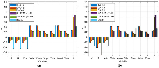
Figure 2.
The -vector for (a) steel and (b) FRP for all load cases.
It is seen that the reliability is, in most cases, larger for FRP than for steel, although the COV on the resistance is 10% for FRP and only 5% for steel. This can happen because the 5% quantile is used as the characteristic value, and a lower value is obtained when the COV is larger. Depending on the importance of this variable, the lower characteristic value may make up for the additional uncertainty. When comparing the -vectors for steel and FRP in Figure 2, it is seen that the resistance variable R is much more important for FRP than for steel.
When comparing the obtained annual reliability indices with the target , it is seen that many values are below the target. If accepting a deviation of 0.1, the reliability level is still too low for DLC 1.1. Here, the same stochastic model was used for DLC 1.3, but a lower safety factor was used for DLC 1.1. Therefore, the reliability index is lower for DLC 1.1, and the -vectors are almost identical.
For the three DLC 6.1 cases, the importance of the load variable L is larger than for DLC 1.1 and 1.3, especially for the typhoon load cases. This is explained by the larger COV for the load for DLC 6.1. However, since the characteristic value is taken as a 98% quantile of the load variable L, the characteristic value also increases. This explains why the reliability index can be slightly larger for DLC 6.1 extreme wind when compared to DLC 1.3 despite the safety factors being the same and the larger uncertainties for DLC 6.1. However, for DLC 6.1 with typhoon loads, the increase in characteristic value is not sufficient to keep the reliability at the same level, and the reliability is only sufficient when the increased safety factor is used but not when the normal safety factor is used.
For gravity loading, there are fewer uncertainties, and the characteristic value of the load is taken as the mean value. Further, the safety factors are smaller than for the remaining load cases. It is seen that this results in larger importance of the variables on the resistance side of the limit state equation, and the reliability index is close to 3.3 for steel. For FRP, the reliability index for gravity loading is less than for steel, whereas it is larger for the remaining load cases. This can be explained by the combination of the increased importance of the resistance variables and the larger uncertainty on the resistance.
The differences in correlation coefficient can be explained by the differences in the importance of the -value for L for the load cases; the higher the -value, the smaller the correlation because the value for L is independent between years, whereas the remaining variables are fully correlated between years.
In Figure 3, the annual reliability index and the cumulative reliability index are shown as a function of time for steel. It is seen that the annual reliability index is almost constant over time for all three DLC 6.1 cases, where the correlation coefficient is quite low. When the annual reliability index is around 3.3, the cumulative reliability index almost drops to = 2.26, as expected for uncorrelated limit states. For DLC 1.1, DLC 1.3, and gravity loading, the annual reliability index increases drastically over time due to the high correlation. This means that the cumulative reliability index ends up being larger compared to the DLC 6.1 cases. For the typhoon load case without increased safety factor, the reliability index is low initially, and the cumulative reliability index after 25 years is the lowest among the considered cases. The high correlation for DLC 1.1, DLC 1.3, and gravity loading also has the effect that the average reliability indices are larger than the target .
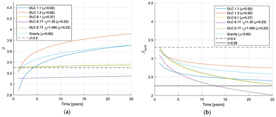
Figure 3.
Reliability index as a function of time for steel, component class 2: (a) annual reliability index; (b) cumulative reliability index.
3.2. Optimal Target Reliability
Initially, an optimization of the reliability index is performed for cost variables , , and , increasing from 0 to 2 using the method described in Section 2.4.
The optimal target reliability is shown as a function of in Figure 4a, and the associated optimal load safety factor is shown in Figure 4b. The dots correspond to optimal values of the design parameter among the ones where reliability analyses were performed, and the lines are obtained by using a cubic smoothing spline on the expected profit Z(z) and then finding the optimal on that spline. DLC 1.1 and DLC 1.3 do not have separate calculations, as only the current safety factor differs, whereas the stochastic models and limit state equations are the same.
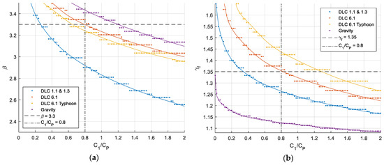
Figure 4.
The optimal value of (a) annual reliability index (in the first year), (b) load safety factor for . The dots correspond to optimal values of the design parameter among the ones where reliability analyses were performed, and the lines are obtained by using a cubic smoothing spline on the expected profit Z(z) and then finding the optimal on that spline.
As it is difficult to assess the value of , a relative assessment is made. It seems appropriate to take DLC 6.1 as the starting point because the failure rate is almost constant over time, and the normal safety factor was found approximately to lead to a reliability index . According to Figure 4a, this target corresponds to the value , and this value is therefore used to find the optimal target reliability and load safety factor, which are shown in Table 4 together with the current values in IEC 61400-1 ed. 4 [5].
Table 4.
Optimal annual target reliabilities and load safety factors.
It is seen that the optimal target reliability for DLC 1.1 and 1.3 is instead of , whereas the optimal safety factor is , which is very close to the current safety factor for DLC 1.1. The lower optimal safety factor can be explained by the fact that the annual reliability index is increasing over time, and thus the cumulative reliability index is still quite large after 25 years, although the initial annual reliability index is lower than for DLC 6.1, as seen in Figure 3.
For DLC 6.1 with typhoon wind, where the coefficient of variation on the annual maximum load is larger, the target reliability is slightly lower (), but a larger safety factor is needed to reach this optimum. Therefore, this target is not reached with the normal safety factor , but the optional increased safety factor given in IEC61400-1 is sufficient [5](pp. 76). For gravity loading, the target reliability is slightly larger (), and the optimal safety factor is close to the value given in the standard .
Figure 5 shows the optimal reliability index and safety factor if the failure costs are increased to . Compared to , the optimal target reliability and safety factor are larger for the same value of . However, if the value of is assessed in a relative way, it is seen that for DLC 6.1 for , and the optimal target reliabilities and safety factors will be almost the same as in Table 4.
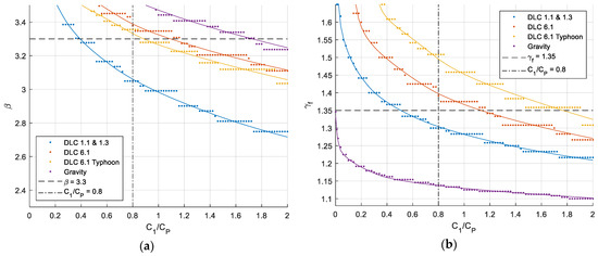
Figure 5.
The optimal value of (a) annual reliability index (in the first year), (b) load safety factor for 0. The dots correspond to optimal values of the design parameter among the ones where reliability analyses were performed, and the lines are obtained by using a cubic smoothing spline on the expected profit Z(z) and then finding the optimal on that spline.
Figure 6 shows the optimal reliability index and safety factor if the discount rate is increased to . It is seen that the target reliabilities become smaller for a fixed value of , because failure consequences, potentially happening in the future, becomes less important when the rate is larger. Moreover, if the relative assessment is made here, a value is found for for DLC 6.1, and the optimal target reliabilities and safety factors will be almost the same as in Table 4.
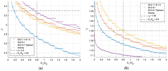
Figure 6.
The optimal value of (a) annual reliability index (in the first year), (b) load safety factor for . The dots correspond to optimal values of the design parameter among the ones where reliability analyses were performed, and the lines are obtained by using a cubic smoothing spline on the expected profit Z(z) and then finding the optimal on that spline.
4. Discussion and Conclusions
This paper aimed to estimate and assess the reliability level for extreme load cases implicitly given through the safety factors in the main design standard for wind turbines IEC 61400-1. The optimal target reliability level was estimated through a relative risk-based comparison with DLC 6.1.
The annual reliability index was found to be close to the target 3.3 (not less than 0.1 below the target) for all considered cases except for DLC 1.1, DLC 6.1 typhoon for steel with the normal safety factor, and gravity for FRP.
For DLC 1.1, this study found a significantly lower annual reliability index than previous studies [17] due to the combined effects of smaller adjustments in the stochastic model between the background document to IEC 61400-1 ed. 4 [17] and IEC CD TS 61400-9 [26]: (1) the uncertainty on the load variable L was smaller in this study, which negatively affects the reliability because the 98% quantile is used as the characteristic value in the design equation; (2) the model uncertainties are assumed slightly larger in this study, as uncertainties previously assumed to be included in L is instead included as a model uncertainty; (3) no bias is assumed on the resistance model.
However, for DLC 1.1, the resistance and model uncertainties dominate, causing the correlation between limit states for different years to be large. Consequently, the cumulative reliability index is not larger than for the other load cases, and the average reliability index is larger than 3.3. The optimal value of the annual reliability index was found to , which corresponds to the value found using the current load safety factor in IEC 61400-1.
For DLC 6.1 with typhoon loads, the annual reliability index was found to , when the normal load safety factor = 1.35 was used. This typically reflects the design, as the typhoon class was introduced in IEC 61400-1 ed. 4 without requirements to use increased safety factors. However, when using the optionally increased safety factor given in a footnote in IEC 61400-1, the annual reliability index was larger than 3.3. For the typhoon case, the load uncertainty dominates, whereby the correlation coefficient between years is low. Therefore, the average reliability index is close to the annual reliability index in the first year, and the cumulative reliability index is low. The optimal annual reliability index is found to be only slightly lower than 3.3, and a larger load safety factor of around 1.44 is needed to achieve this. However, this assumes a linear relationship between the costs and the resistance. If the demands for a resistance sufficient for typhoon loads require more radical design changes (resulting in a larger factor ), this could motivate lower target reliability, and a lower safety factor could be sufficient.
For the DLCs where it is found that the reliability implicitly given through the safety factors is less than the target , the use of probabilistic methods directly with the target may lead to a more expensive design. If the target reliability level was optimal based on economic risk-based considerations, then this more expensive design was more optimal because it gives the optimal balance between the failure risks and the costs of improving the reliability. However, we demonstrated through a relative risk-based comparison between different load cases with extreme loads that lower target reliability could be motivated for DLC 1.1, and this would correspond to the reliability level implicitly given through the safety factors in IEC 61400-1.
Therefore, lower annual target reliability could also be used for probabilistic designs according to IEC TS 61400-9 for DLC 1.1. This could be formulated as a reduced annual target reliability, as a lifetime reliability index, or it could be allowed to compare the average annual reliability index with the current target. It seems preferable to continue using annual target reliabilities, as they are least sensitive to the design lifetime. A reduced target for the annual failure probability would be easiest for the designer, as they would only need to calculate the annual failure probability. From a theoretical perspective, the most direct would be to allow the target to be compared to the average annual reliability index corresponding to the asymptotic renewal density, as suggested originally by Rackwitz [22].
However, challenges arise concerning through-life integrity management, where the reliability can be updated continuously based on inspections and monitoring data and where decisions can be made related to operations and maintenance. Potentially, the use of a reduced target in this context could lead to decisions that are not optimal, and this aspect should be considered carefully.
Author Contributions
Conceptualization, J.S.N., H.S.T. and G.O.V.; methodology, J.S.N.; writing—original draft preparation, J.S.N.; writing—review and editing, H.S.T. and G.O.V. All authors have read and agreed to the published version of the manuscript.
Funding
The work on this paper has been supported by the Danish Energy Agency through the EUDP ProbWind (Grant Number 64019-0587). The support is greatly appreciated.
Data Availability Statement
Not applicable.
Conflicts of Interest
The authors declare no conflict of interest. The funders had no role in the design of the study; in the collection, analyses, or interpretation of data; in the writing of the manuscript; or in the decision to publish the results.
References
- Wang, Z.; Zeng, T.; Chu, X.; Xue, D. Multi-Objective Deep Reinforcement Learning for Optimal Design of Wind Turbine Blade. Renew. Energy 2023, 203, 854–869. [Google Scholar] [CrossRef]
- Yang, K.; Deng, X. Layout Optimization for Renovation of Operational Offshore Wind Farm Based on Machine Learning Wake Model. J. Wind Eng. Ind. Aerodyn. 2023, 232, 105280. [Google Scholar] [CrossRef]
- Zhang, C.; Long, K.; Zhang, J.; Lu, F.; Bai, X.; Jia, J. A Topology Optimization Methodology for the Offshore Wind Turbine Jacket Structure in the Concept Phase. Ocean Eng. 2022, 266, 112974. [Google Scholar] [CrossRef]
- Ziegler, L.; Rhomberg, M.; Muskulus, M. Design Optimization with Genetic Algorithms: How does Steel Mass Increase if Offshore Wind Monopiles are Designed for a Longer Service Life? J. Phys. Conf. Ser. 2018, 1104, 012014. [Google Scholar] [CrossRef]
- IEC 61400-1 ed. 4; Wind Energy Generation Systems—Part 1: Design Requirements. International Electrotechnical Commision: Geneva, Switzerland, 2019.
- Jiang, Z.; Hu, W.; Dong, W.; Gao, Z.; Ren, Z. Structural Reliability Analysis of Wind Turbines: A Review. Energies 2017, 10, 2099. [Google Scholar] [CrossRef]
- Sørensen, J.D.; Frandsen, S.; Tarp-Johansen, N.J. Effective Turbulence Models and Fatigue Reliability in Wind Farms. Probabilistic Eng. Mech. 2008, 23, 531–538. [Google Scholar] [CrossRef]
- Velarde, J.; Kramhøft, C.; Sørensen, J.D.; Zorzi, G. Fatigue Reliability of Large Monopiles for Offshore Wind Turbines. Int. J. Fatigue 2020, 134, 105487. [Google Scholar] [CrossRef]
- Velarde, J.; Mankar, A.; Kramhøft, C.; Sørensen, J.D. Probabilistic Calibration of Fatigue Safety Factors for Offshore Wind Turbine Concrete Structures. Eng. Struct. 2020, 222, 111090. [Google Scholar] [CrossRef]
- Tarp-Johansen, N.J. Partial Safety Factors and Characteristic Values for Combined Extreme Wind and Wave Load Effects. J. Sol. Energy Eng. 2005, 127, 242–252. [Google Scholar] [CrossRef]
- Agarwal, P.; Manuel, L. Implied Reliability Levels in Different Load Models for Offshore Wind Turbines. In Proceedings of the International Conference on Offshore Mechanics and Arctic Engineering, San Francisco, CA, USA, 8–13 June 2014; American Society of Mechanical Engineers (ASME): New York, NY, USA, 2014; Volume 45547, p. V09BT09A051. [Google Scholar]
- Augustyn, D.; Ulriksen, M.D.; Sørensen, J.D. Reliability Updating of Offshore Wind Substructures by Use of Digital Twin Information. Energies 2021, 14, 5859. [Google Scholar] [CrossRef]
- Nielsen, J.S.; Tcherniak, D.; Ulriksen, M.D. A Case Study on Risk-Based Maintenance of Wind Turbine Blades with Structural Health Monitoring. Struct. Infrastruct. Eng. 2020, 17, 302–318. [Google Scholar] [CrossRef]
- Slot, R.M.M.; Sørensen, J.D.; Sudret, B.; Svenningsen, L.; Thøgersen, M.L. Surrogate Model Uncertainty in Wind Turbine Reliability Assessment. Renew. Energy 2020, 151, 1150–1162. [Google Scholar] [CrossRef]
- Schröder, L.; Dimitrov, N.K.; Verelst, D.R.; Sorensen, J.A. Wind Turbine Site-Specific Load Estimation using Artificial Neural Networks Calibrated by means of High-Fidelity Load Simulations. J. Phys. Conf. Ser. 2018, 1037, 062027. [Google Scholar] [CrossRef]
- JCSS. Risk Assessment in Engineering—Principles, System Representation & Risk Criteria; Joint Commitee on Structural Safety: Deift, The Netherlands, 2008. [Google Scholar]
- Sørensen, J.D.; Toft, H.S. Safety Factors—IEC 61400-1 ed. 4—Background Document; DTU Energy Department of Wind Energy: Roskilde, Denmark, 2014; Volume 0066. [Google Scholar]
- ISO2394; General Principles on Reliability for Structures. International Organization for Standardization: Geneva, Switzerland, 2015.
- Köhler, J.; Sørensen, J.D.; Baravalle, M. Calibration of Existing Semi-Probabilistic Design Codes. In Proceedings of the 13th International Conference on Applications of Statistics and Probability in Civil Engineering, ICASP 2019, Seoul, Republic of Korea, 26–30 May 2019; p. 325. [Google Scholar]
- Al-Sanad, S.; Wang, L.; Parol, J.; Kolios, A. Reliability-Based Design Optimisation Framework for Wind Turbine Towers. Renew. Energy 2021, 167, 942–953. [Google Scholar] [CrossRef]
- Nielsen, J.S.; Sørensen, J.D. Risk-Based Derivation of Target Reliability Levels for Life Extension of Wind Turbine Structural Components. Wind Energy 2021, 24, 939–956. [Google Scholar] [CrossRef]
- Rackwitz, R. Optimization—The Basis of Code-Making and Reliability Verification. Struct. Saf. 2000, 22, 27–60. [Google Scholar] [CrossRef]
- JCSS. Probabilistic Model Code; JCSS: Deift, The Netherlands, 2001. [Google Scholar]
- Fischer, K.; Viljoen, C.; Köhler, J.; Faber, M.H. Optimal and Acceptable Reliabilities for Structural Design. Struct. Saf. 2019, 76, 149–161. [Google Scholar] [CrossRef]
- Nielsen, J.S.; Miller-Branovacki, L.; Carriveau, R. Probabilistic and Risk-Informed Life Extension Assessment of Wind Turbine Structural Components. Energies 2021, 14, 821. [Google Scholar] [CrossRef]
- IEC CD TS 61400-9; Wind Energy Generation Systems—Part 9: Probabilistic Design Measures for Wind Turbines. International Electrotechnical Commission: Geneva, Switzerland, 2023.
- Simiu, E.; Heckert, N.A.; Filliben, J.J.; Johnson, S.K. Extreme Wind Load Estimates Based on The Gumbel Distribution of Dynamic Pressures: An Assessment. Struct. Saf. 2001, 23, 221–229. [Google Scholar] [CrossRef]
- Thoft-Christensen, P.; Sørensen, J.D. Reliability of Structural Systems with Correlated Elements. Appl. Math. Model. 1982, 6, 171–178. [Google Scholar] [CrossRef]
- Straub, D.; Der Kiureghian, A. Reliability Acceptance Criteria for Deteriorating Elements of Structural Systems. J. Struct. Eng. 2011, 137, 1573–1582. [Google Scholar] [CrossRef]
- Mendoza, J.; Nielsen, J.S.; Sørensen, J.D.; Köhler, J. Structural Reliability Analysis of Offshore Jackets for System-Level Fatigue Design. Struct. Saf. 2022, 97, 102220. [Google Scholar] [CrossRef]
- Madsen, H.O.; Krenk, S.; Lind, N.C. Methods of Structural Safety; Dover Publications: Mineola, NY, USA, 2006; ISBN 0-486-44597-6. [Google Scholar]
Disclaimer/Publisher’s Note: The statements, opinions and data contained in all publications are solely those of the individual author(s) and contributor(s) and not of MDPI and/or the editor(s). MDPI and/or the editor(s) disclaim responsibility for any injury to people or property resulting from any ideas, methods, instructions or products referred to in the content. |
© 2023 by the authors. Licensee MDPI, Basel, Switzerland. This article is an open access article distributed under the terms and conditions of the Creative Commons Attribution (CC BY) license (https://creativecommons.org/licenses/by/4.0/).