An Aero-Structural Model for Ram-Air Kite Simulations

Abstract

Similar to parafoils, ram-air kites are flexible membrane wings inflated by the apparent wind and supported by a bridle line system. A major challenge in estimating the performance of these wings using a computer model is the strong coupling between the airflow around the wing and the deformation of the membrane structure. In this paper, we introduce a staggered coupling scheme combining a structural finite element solver using a dynamic relaxation technique with a potential flow solver. The developed method proved numerically stable for determining the equilibrium shape of the wing under aerodynamic load and is thus suitable for performance measurement and load estimation. The method was validated with flight data provided by SkySails Power. Measured forces on the tether and steering belt of the robotic kite control pod showed good resemblance with the simulation results. As expected for a potential flow solver, the kite’s glide ratio was overestimated by 10–15%, and the measured tether elevation angle in a neutral flight scenario matched the simulations within 2 degrees. Based on the obtained results, it can be concluded that the proposed aero-structural model can be used for initial designs of ram-air kites with application to airborne wind energy.

1. Introduction

The growing energy demand and shift toward carbon-free electricity production is rapidly expanding the market for renewable energies [1]. While most countries are forced to adapt their production accordingly, the demand for renewable energy also opens the field for alternative wind energy technologies. Airborne wind energy (AWE) is such an alternative approach that is aimed at harvesting wind from higher altitudes using tethered flying devices [2]. Next to the potential of accessing an additional source of renewable energy, a key motivating factor is the substantially lower material footprint of the technology. Several different system configurations have been tested so far. SkySails Power developed a ground-based airborne wind energy system that uses a ram-air kite to drive an electrical generator. During the power phase, the kite is flown in figure-eight maneuvers, pulling the tether off a drum that is coupled to a generator. When the maximum tether length is reached, the kite is depowered to reduce its pulling force. After a transfer phase, the kite is pulled toward the ground station using the generator as a motor. Once the kite has reached its initial position, the power cycle is repeated. Methods for estimating the performance of such pumping AWE systems have been presented in [3,4,5,6]. For more detailed information regarding AWE system configurations, refer to [7,8].

Ram-air kites and parafoils are made of thin woven fabric and are inflated by the airflow entering the wing through intakes located at the kite’s leading edge [9,10,11,12]. The aerodynamic shape of the wing is defined by internal ribs similar to the ribs in an aircraft wing and bridle lines that attach to the ribs and transmit the forces from the wing to the tether [13]. Ram-air wings for AWE applications are designed to produce maximum tether force during the reel-out phase and have to withstand these loads for many power cycles. To better predict the aerodynamic loads on the wing and the resulting—often large—deformations, an accurate numerical simulation of the fluid-0structure interaction (FSI) process is indispensable.

Several aero-elastic models for ram-air kites have been developed in the past. A complete dynamic approach with a staggered FSI scheme was proposed by Ortega et al. [14] consisting of a cost-effective low-fidelity potential flow solver with deforming wake and an explicit dynamic solver with a wrinkling model and viscous damping to determine the wing shape. The intake flow was not modeled because of the limitations of potential flow. The solver was tested on a free-flying parachute payload configuration with and without deflecting steering lines. The comparison of the computed and measured flight velocity and glide ratio showed a satisfactory agreement.

A three-dimensional FSI analysis, including the intake flow, was conducted by Fogell et al. [15,16]. They investigated the aeroelastic deformation of a single wing section during steady gliding flight using a loosely coupled approach. The fluid dynamics were solved with the commercial fluid solver STAR-CCM using the Reynolds-Averaged Navier–Stokes (RANS) approach. The structural response was modeled with linear elastic isotropic material properties using the commercial software LS-DYNA.

Lolies et al. [17] studied the dynamics of a paraglider using a high-fidelity transient FSI simulation based on an immersed boundary coupling approach. The flow was simulated with a lattice Boltzmann method, and the structural model consisted of an arrangement of elastic springs allowing larger time steps for the transient time integration. The computed shape of the parafoil agreed with the shape measured in the wind tunnel, but an underresolved boundary layer caused by the immersed boundary method was observed.

Folkersma et al. [18] modeled a ram-air kite by coupling RANS simulations with OpenFOAM to determine the aerodynamic pressure distribution on the wing surface with the FEM solver mem4py [19] to compute the resulting deformations of the membrane structure. The framework was used to compute the steady-state shape of the wing for several trim configurations. In the present paper, a similar technique is used to determine the steady-state shape for a single trim configuration. However, instead of using CFD, a faster potential flow solver is employed to determine the aerodynamic surface pressure distribution.

The paper summarizes the PhD research of the first author [20] and is organized as follows. In Section 2, the coupling scheme is introduced. The assumptions to justify a steady-state behavior of the kite are critically reflected on, and the solver framework is verified for the same kite as used in [18]. In Section 3, there is a description of how the developed FSI solver is applied to a 120 m${}^2$ ram-air kite designed by SkySails Power. The tether and steering belt forces and the glide ratio are compared to data measured during a 42 h flight. Additionally, the elevation angle during a neutral flight state is compared to a three-minute flight window. Finally, the results are concluded in Section 4.

2. Methodology

Modeling the aeroelastic behavior of a tethered soft kite flying in a turbulent wind environment poses a number of challenges. In this section, we introduce the relevant assumptions to simplify the physical problem and develop a simulation approach.

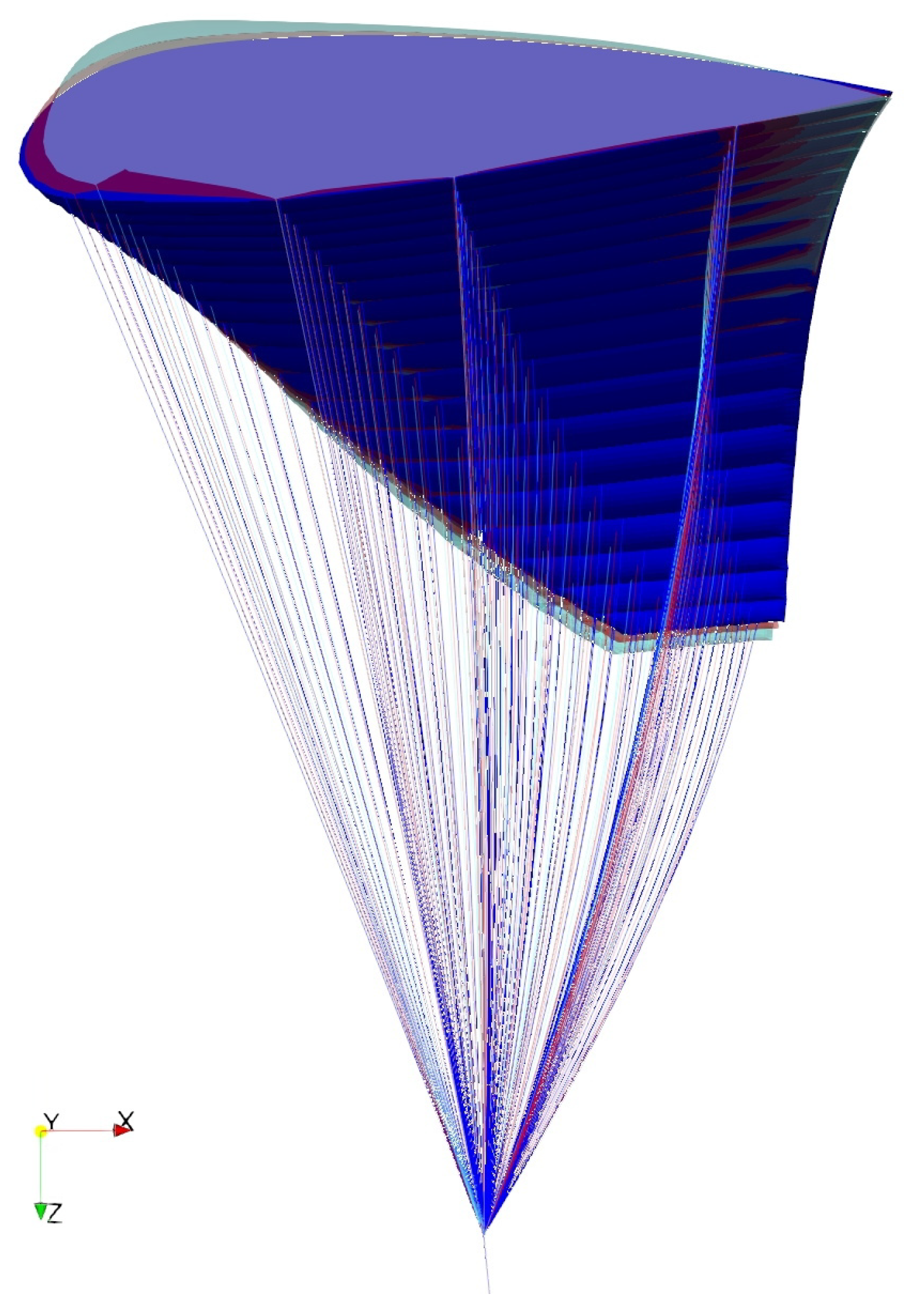
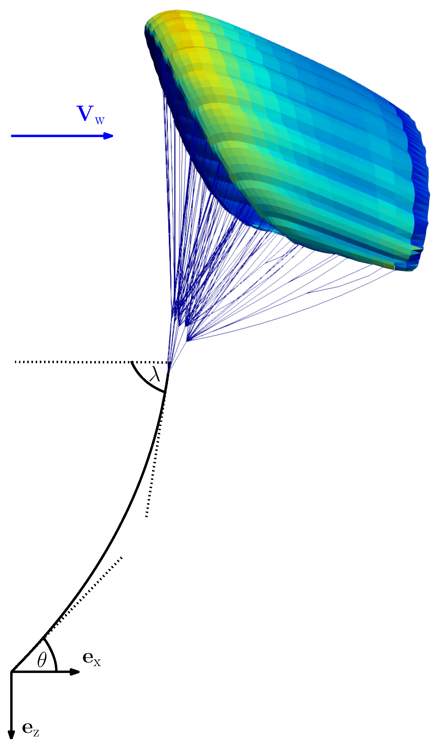
2.1. Simulation Setup–Virtual Wind Tunnel and Model Assumptions

The aerodynamic and structural characteristics of the parafoil, such as the glide ratio, the tether and bridle line forces, and the mechanical stresses are determined in a virtual wind tunnel environment that reproduces realistic flight conditions. The power harvesting envelope of a SkySails Power parafoil consists of four phases: the power, transfer, retraction, and restart phases [21]. During the power phase, the kite is flown in crosswind figure-eight maneuvers at relatively low-elevation angles to produce a maximum tether tension. At the same time, the winch reels out the tether, modulates the speed, and also controls the apparent wind speed at the kite and the tether force. To avoid modeling a whole figure-eight trajectory with steering input and transient aerodynamic and structural effects, a steady flight state is assumed between two turning maneuvers when the parafoil reaches a constant flight velocity and inflow angle, as depicted in Figure 1a. This steady-state flight is defined by an equilibrium of all forces acting on the kite: the distributed aerodynamic load, the gravitational forces, and the tether force. The equilibrium state during steady-state flight provides valuable insight into the coupled aerodynamic and structural characteristics of the kite.

Figure 1b depicts the influence of gravity on the airborne system components, which cause the tether to sag toward the ground and require a small part of the lift force of the kite to compensate for the effect of gravity on the tether and kite.

Consequently, the tension in the tether is slightly reduced, and the tether elevation angle at the kite is slightly larger than the elevation angle at the ground, with both values deviating from the geometric elevation angle [6]. For an AWE system utilizing soft kites, the weight of the parafoil and tether is less than 1% of the average tether force during the power phase, and, therefore, the influence of gravity can be neglected during the power phase, which allows for the use of a symmetry condition as explained later. On the other hand, tether sag due to aerodynamic drag is accounted for in the model.

The apparent wind velocity vector experienced by the kite is defined as follows:

$${\mathbf{V}}_{\mathrm{a}}={\mathbf{V}}_{\mathrm{w}}-{\mathbf{V}}_{\mathrm{k}},$$

(1)

where ${\mathbf{V}}_{\mathrm{w}}$ is the wind velocity and ${\mathbf{V}}_{\mathrm{k}}$ is the flight velocity of the kite. The latter can be further decomposed into a component ${\mathbf{V}}_{\mathrm{k},\tau }$ perpendicular to the tether and a component ${\mathbf{V}}_{\mathrm{k},\mathrm{r}}$ aligned with the tether, which for a straight tether, is identical to the tether reeling velocity ${\mathbf{V}}_{\mathrm{t}}$ at the ground [22]. The velocities acting on the kite during crosswind flight are illustrated in Figure 2a.

The angle $\vartheta$ is measured between the wind velocity vector ${\mathbf{V}}_{\mathrm{w}}$ and the tether, while the angle $\varphi$ is measured in the $yz$-plane of the wind reference frame between the vertical and the orthogonal projection of the kite position. Figure 2b shows the definition of the apparent wind velocity, the angle of attack, and the aerodynamic forces acting on the kite. For a kite performing crosswind maneuvers in a uniform wind field, the apparent wind speed along the tether varies linearly [23]. However, a realistic wind field is always nonuniform, with the magnitude and orientation of the velocity vector varying in both space and time. Also, the flight speed of the kite depends on the resultant glide ratio of all airborne components, which varies with the paid-out length of the tether and the flight altitude of the kite. For a simplified analysis of crosswind flight, the inflow velocity ${\mathbf{V}}_{\mathrm{a}}$ is assumed to be linearly varying along the tether.

Figure 3 depicts the initial condition of the virtual wind tunnel setup with a horizontal, linearly varying inflow and a vertical tether connecting via a bridle line system to the undeformed parafoil.

For the simplified steady-state flight condition with neglected gravitational effects, only half of the wing is modeled, which exploits the symmetry of the FSI problem with respect to the center rib of the parafoil. This also means that no steering input can be applied in the simulation. During the coupling iterations, the kite translates and pitches from this initial position and orientation until it eventually assumes an equilibrium state, where the aerodynamic forces are balancing the tether force. This final state corresponds to the trim condition of the parafoil with the angle of attack at its trim value. To illustrate this, Figure 4 compares the initial configuration and shape of the kite for two different positions ${\delta }_1$ and ${\delta }_2$ of the bridle point with the shapes in steady-state flight, resulting in two different trim values ${\alpha }_1$ and ${\alpha }_2$ of the angle of attack [18].

To avoid a front stall of the parafoil in the first coupling iteration, which would produce a negative lift and a collapse due to a low angle of attack, a minimum angle of attack ${\alpha }_0$ is set as an initial value.

The distributed aerodynamic load on the kite is computed with the open source tool APAME, which is a potential flow solver based on the panel method [24]. For computing the deformation of the inflated membrane structure and the connected bridle lines, the open source tool mem4py is used [19,20]. This in-house FEM solver was specifically developed for fabric membrane structures and is based on the kinetic dynamic relaxation method introduced in [25,26]. To correct the compressive stress state in each membrane element, a wrinkling model valid for orthotropic materials is used [27].

2.2. Force Coefficients and Glide Ratio

The structural force distribution in the kite can be characterized by the tether and steering belt forces, ${\mathbf{F}}_{\mathrm{tether}}$, ${\mathbf{F}}_{\mathrm{belt},\mathrm{left}}$ and ${\mathbf{F}}_{\mathrm{belt},\mathrm{right}}$, respectively [9]. Figure 5 shows a photo of the SkySails Power system during takeoff and a schematic close-up of the control pod, indicating where these three forces are measured with load cells.

Since the control pod is not modeled, the resultant force acting in the bridle lines that are not connected to the steering belt can be determined as follows:

$${\mathbf{F}}_{\mathrm{bridle}}=-\left({\mathbf{F}}_{\mathrm{tether}}+{\mathbf{F}}_{\mathrm{belt},\mathrm{left}}+{\mathbf{F}}_{\mathrm{belt},\mathrm{right}}\right).$$

(2)

From the dimensional values, the following nondimensional coefficients are derived

$$\begin{array}{cc}\hfill C_{\mathrm{R}}& =\frac{F_{\mathrm{tether}}}{\frac{1}{2}\rho V_{\mathrm{a}}^{2}S},\hfill \end{array}$$

(3)

$$\begin{array}{cc}\hfill C_{\mathrm{B}}& =\frac{F_{\mathrm{belt}}}{\frac{1}{2}\rho V_{\mathrm{a}}^{2}S},\hfill \end{array}$$

(4)

where $\rho$ is the air density, and S is the projected wing surface area.

The resultant aerodynamic lift and drag forces acting on the kite are determined by integrating the aerodynamic surface pressure distribution $p_{\mathrm{a}}$, overall membrane elements, and the aerodynamic line drag over all bridle line elements. The glide ratio E can then be evaluated as the ratio $L/D$ of lift and drag forces. It should be noted that the surface pressure $p_{\mathrm{i}}$ on the inside of the membrane elements is not computed with the potential flow solver but assumed to be uniform and identical to the stagnation pressure at the inflow opening of the wing. This is a reasonable assumption for ram-air wings because the flow speeds in the enclosed volume are relatively low since the air can escape only through the permeable fabric, seams, and other leakage options. With $p_{\mathrm{i}}=p_{\infty }+1/2\rho V_{\mathrm{a}}^2$, the resultant pressure coefficient can then be computed as follows:

$$C_{\mathrm{p}}=\frac{p_{\mathrm{a}}-p_{\infty }}{\frac{1}{2}\rho V_{\mathrm{a}}^2}-\frac{p_{\mathrm{i}}-p_{\infty }}{\frac{1}{2}\rho V_{\mathrm{a}}^2}=C_{\mathrm{p},\mathrm{a}}-1,$$

(5)

where $C_{\mathrm{p},\mathrm{a}}$ is the pressure coefficient determined by the potential flow solver and $p_{\infty }$ the static pressure in the far field.

2.3. Coupling Algorithm

The interface coupling of fluid and structure solvers is outlined with Algorithm 1.

The coupling tool preCICE [28] initializes the communication between the solvers and in each iteration, interpolates all field variables between the two interfaces. Due to the steady flight assumption, the coupling iterations occur in a single pseudo time step, and either explicit or implicit coupling methods can be used to find the equilibrium state. In case of explicit coupling, no information of the previous iteration is used, the pressure is given to the FEM, and the displacements are handed back to the panel code until convergence in the displacement is reached. In case of implicit coupling, the IQN-ILS approached proved to perform better for some kite geometries than did the explicit method. In the implicit approach, an implicit least-squares method (ILS) is used to approximate the relation between pressure and displacement within a single time step. The difference between the implicit and explicit coupling is that for the implicit approach, the displacement vector is scaled by the least-squares method (see line 13 in Algorithm 1), whereas for the explicit method, no scaling is applied, and the first iteration of both approaches is equivalent. A growing difference between both interfaces defines divergent coupling behavior, and it usually results in an wing flying upside down, which is indicated by a negative lift coefficient. Hence, the simulation is aborted if $C_{\mathrm{L}}<0$. For the kite geometries used in this work, the total number of coupling iterations varied between 10 and 60. It was observed that a higher mesh resolution also resulted in more coupling iterations because the kite would show more local deformation details that had an influence on the convergence. Also, the kite model provided by SkySails would converge only when using the implicit coupling approach.

Algorithm 1 FSI coupling procedure.

1: Read structure and fluid mesh. 2: Initialize displacement field $\mathbf{u}$ and surface pressure field p. 3: Set iteration counter $i=1$. 4: while ||${\mathbf{u}}_i$ − ${\mathbf{u}}_{i-1}$||>${\epsilon }_{\mathrm{FSI}}$ do. 5:       if $C_{\mathrm{L}}$ < 0 then 6:             break 7:       end if 8:       Run APAME on geometry with deformation field ${\mathbf{u}}_i$. 9:       Correct $C_{\mathrm{p}}$ distribution with internal pressure using Equation (5). 10:     Pass $C_{\mathrm{p}}$ distribution to mem4py. 11:     Run mem4py with current pressure distribution. 12:     $i=i+1$. 13:     Pass ${\mathbf{u}}_i$ back to APAME. For implicit coupling scale ${\mathbf{u}}_i$. 14: end while 15: Postprocessing

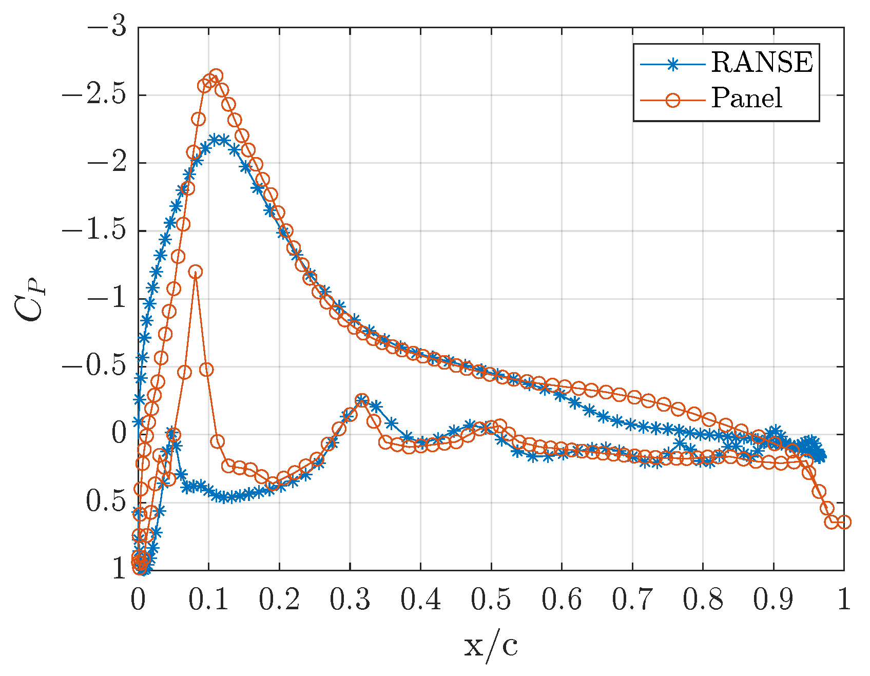
2.4. Solver Verification

For verification, the developed FSI solver was used to simulate the ram-air kite with an 160 m${}^2$ flat (laid-out) wing surface area that was investigated in [18]. Figure 6 illustrates the computed shapes of the half-kite for typical apparent wind speeds $V_{\mathrm{a}}$ = 10, 20, and 30 m/s.

While a small change in the profile shape could already be observed when the speed was increased from 10 to 20 m/s, an increase to 30 m/s led to a strong shape deformation of the leading edge, which in return affected the aerodynamics of the wing.

In a next step, the computed aerodynamic coefficients and pressure distributions were compared with the results presented in [18]; it is important to note that in this earlier study, only the aerodynamic solver was different, with the CFD solver OpenFOAM being used instead of the panel method APAME. The FEM solver and coupling procedure were identical. Figure 7a,b show the lift and drag coefficients as functions of the angle of attack at the center rib.

It can be seen that both coefficients exhibited a similar trend until larger angles of attack, where the RANS solution (Folkersma et al 2020 [18]) started to drop in lift as a result of flow separation. As expected, the potential flow stayed attached to the wing without reduction of the lift at high angles of attack. The drag coefficient showed a good match between the two solutions for angles of attack smaller than 15 degrees when both curves started to deviate.

Figure 7c,d show the resultant force coefficient and glide ratio as functions of the angle of attack. The $C_{\mathrm{R}}\left(\alpha \right)$ and $C_{\mathrm{L}}\left(\alpha \right)$ functions are very similar, which emphasizes the importance of a high lift for generating a high pulling force as the $C_{\mathrm{L}}$ contribution to $C_{\mathrm{R}}$ dominates by a factor of 5 to 10 depending on the angle of attack. For the comparison of the glide ratio of both approaches, a good match except for low angles of attack of around 5 degrees can be seen despite the differences in lift and drag.

In Figure 8, the resultant pressure coefficient along the chord of the center rib is presented, computed for a trim configuration with $\delta =42\%$.

Despite an identical bridle configuration, the trim angle of attack in the RANS simulation is 12.4 degrees, whereas the value computed with the panel method is 14.8 degrees. The $C_{\mathrm{p}}$-distributions have a similar appearance. The panel method exhibits a steeper slope over the first 10% of the chord, and the pressure peak is only half of that observed in the RANS simulation. Also, the line attachment points create a kink in the parafoil shape to which both solvers react with a local pressure drop. This drop is particularly pronounced for the panel method, leading to larger angles between neighboring panels.

It can be concluded that the panel method can approximate the pressure field fairly well compared to the RANS simulation. Care should be taken for large deformations that can cause strong and even nonphysical local pressure drops. As an initial design tool for parafoils, the panel method allows for efficient and relatively accurate determination of the aerodynamic surface pressure distribution without the generally extensive preprocessing effort to generate high-quality volume meshes for CFD and the long simulation times. Aerodynamic parameters like lift and drag are approximated within a 30% difference for a range of angles of attack. Nevertheless, it should be emphasized that the definition of an angle of attack for soft kites is not trivial due to possible chord deformation and rotation [29]. A better way to compare the solutions is the trim position defined on the undeformed kite geometry (see Figure 4).

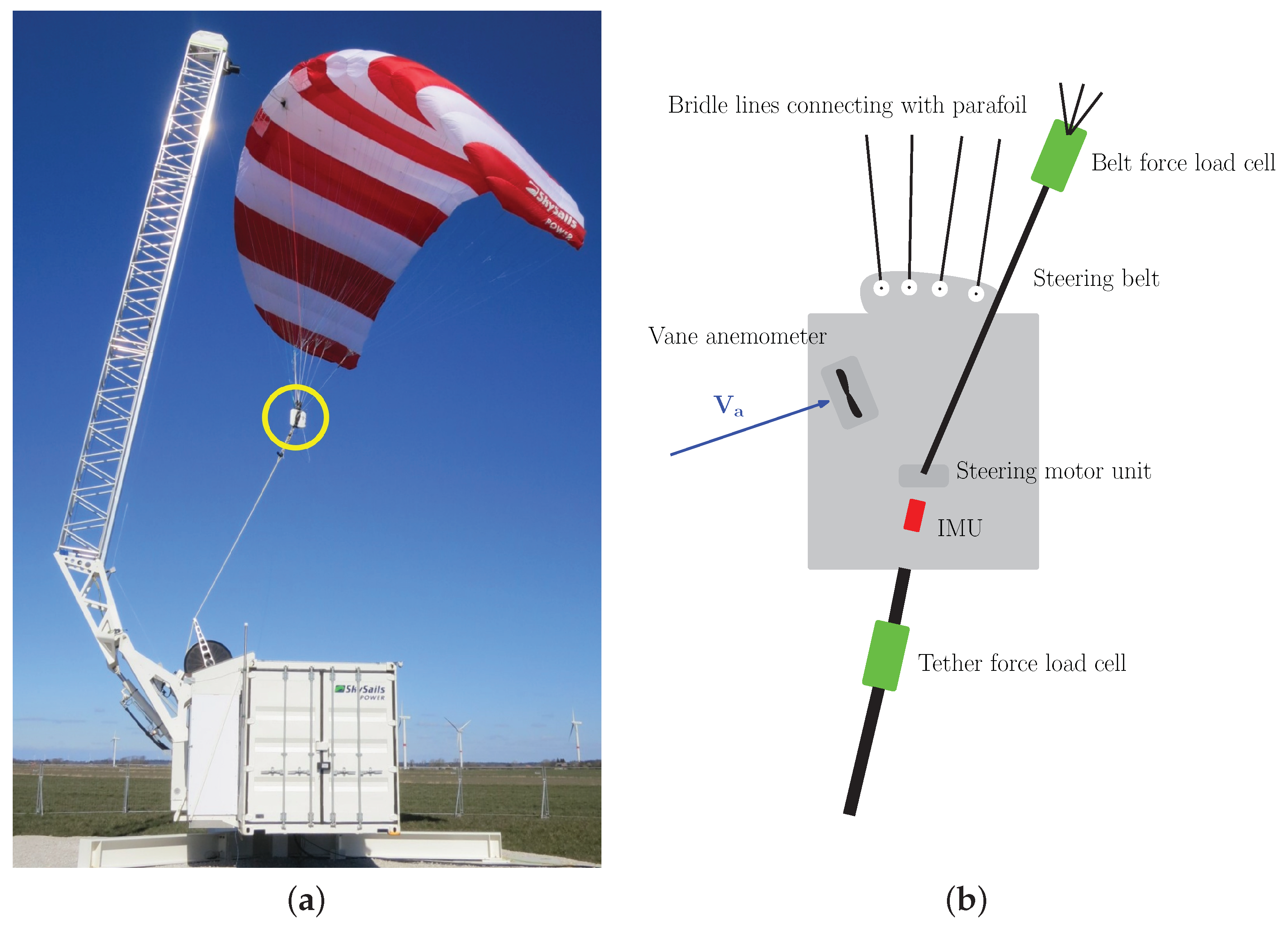
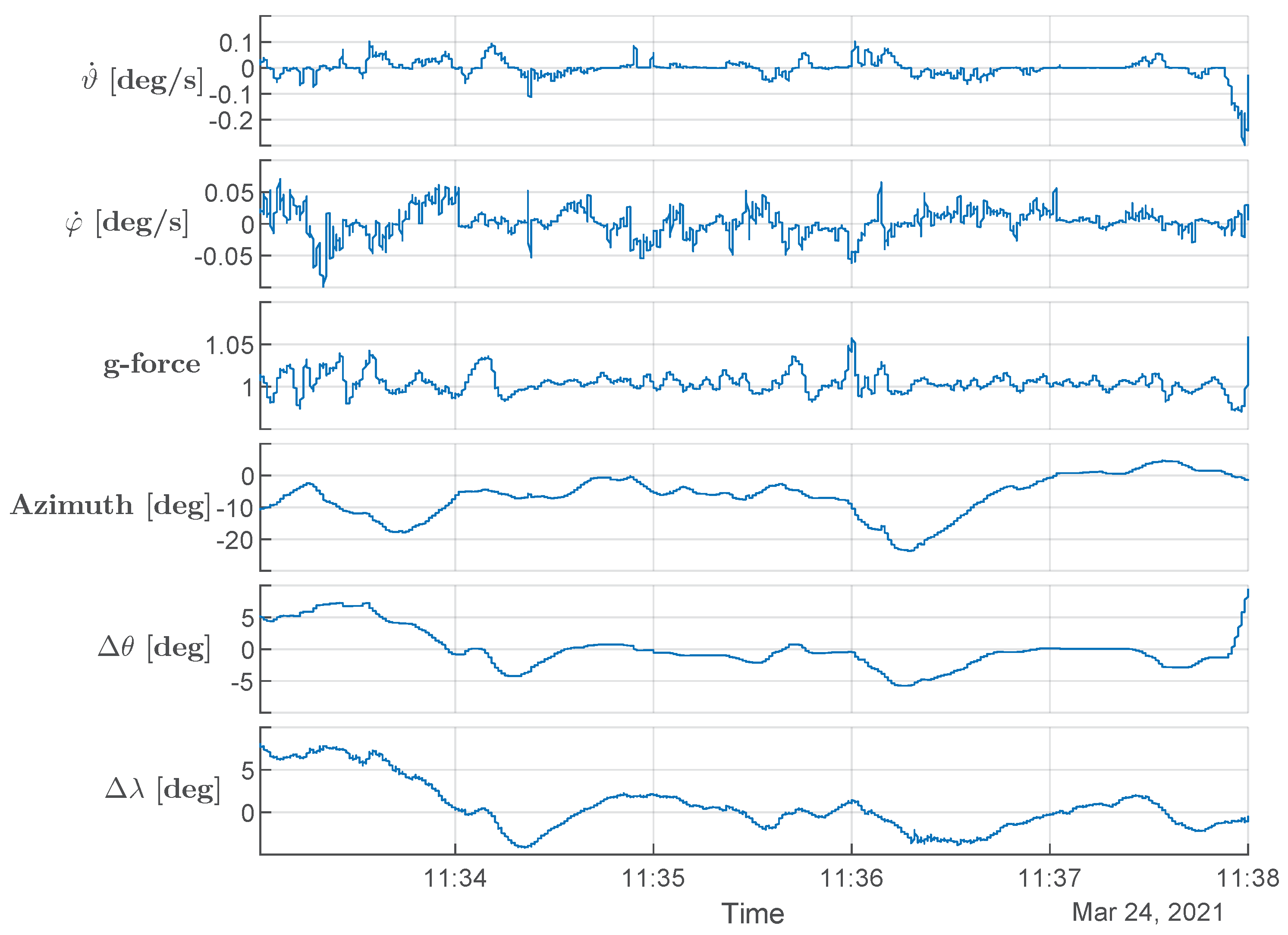
2.5. Measurement Setup, Data Acquisition, and Postprocessing

The instrumentation of the control pod is detailed in Figure 5. Next to force and apparent wind speed at the kite, the tether angles $\vartheta$ and $\varphi$, as defined in Figure 2a, were measured with a LIDAR, as was the vertical wind profile. The instrumentation of the system was similar to the setup described in Erhard et al. [30].

The tensile forces in the bridle line system, $F_{\mathrm{tether}}$, $F_{\mathrm{belt},\mathrm{left}}$, and $F_{\mathrm{belt},\mathrm{right}}$, were measured with three load cells. These data were recorded at a frequency of 10 Hz and were synchronized during flight. The instruments were calibrated before the flight using a tension test machine and proved to be reliable for many flight hours.

The apparent wind speed at the kite was recorded with two vane anemometers attached to the sides of the control pod, as indicated in Figure 5b. Because the anemometers were aligned with the roll axis of the kite, they in fact only measured the component of the velocity along this axis. In Figure 2b, this measured velocity component can be identified as $V_{\mathrm{a},\tau }$ and is related to the apparent wind speed $V_{\mathrm{a}}$ as follows:

$$\frac{V_{\mathrm{a},\tau }}{V_{\mathrm{a}}}=\frac{L_{\mathrm{K}}}{\sqrt{L_{\mathrm{K}}^2+D_{\mathrm{K}}^2}}.$$

(6)

This fundamental equation is based on the geometric similarity of the velocity and force triangles, linking the kinematics of the relative flow at the kite to the decomposition of the resultant aerodynamic force [22]. Equation (6) can be used to correct for the misalignment of the anemometer with the local inflow vector:

$$V_{\mathrm{a}}=V_{\mathrm{a},\tau }\sqrt{\frac{1+E^2}{E^2}},$$

(7)

where E is the parafoil’s glide ratio. During the retraction phase and turning maneuvers, the angle of attack can vary significantly, which leads to erroneous deviations of $V_{\mathrm{a}}$ because the misalignment correction uses a constant glide ratio. To reduce such inaccurate measurements, only the power and transfer phases were considered for validation when the kite was not steered, and the tether sag was small due to a high apparent velocity and pulling force. The manufacturer calibrated the vane anemometers, and before the flight, a new set of propellers was attached. Not measuring the angle of attack and the apparent wind speed directly is a clear disadvantage of the described method. Also, the control pod influences the airflow around the vane anemometers, such that the measured apparent wind speed deviates to some degree from the actual speed. Because of this disturbance effect and the error introduced when using the misalignment correction with a constant glide ratio, uncertainty remains in determining $V_{\mathrm{a}}$ during flight.

The tether angles $\vartheta$ and $\varphi$, as defined in Figure 2a, were measured at the ground station with line angle sensors. Together with the recorded length of the reeled out tether, this allowed for the estimation of the position of the kite during the power phase. It was also possible to measure the angle between the tether and the control pod and use this to improve the $\vartheta$-estimate. The control pod was also equipped with an inertial measurement unit (IMU) to determine the accelerations in three axes such that both the orientation and turn rates of the kite system could be derived.

The glide ratio of the kite, defined as the assembly of the wing, bridle line system, and control pod, was not directly measured but estimated from the quasi-steady theory of tethered flight, using the following equation: [30]

$$E=\frac{V_{\mathrm{a}}}{V_{\mathrm{w}}cos\vartheta -V_{\mathrm{t}}},$$

(8)

where $\vartheta$ is the angle between the wind velocity vector and the tether, as indicated in Figure 2a. Equation (8) is valid for a negligible effect of gravity and a glide ratio $E\gg 1$, which is common for AWE applications.

The following data filtering and selection procedures were applied to the raw flight test data:

• The data were smoothed with a 3 s moving average to level out short-term fluctuations using the Matlab function movmean. It was found that this procedure provided a good smoothing behavior without influencing the measurement over a power cycle.
• The symmetry assumption of the parafoil was enforced by selecting only data points during the straight flight when the steering belt position was not further than 5 cm from the neutral position in both directions.
• To enforce the quasi-steady flight assumption, the magnitude of the measured acceleration during the flight was used to select data points which satisfied a $0.1$ g offset.

3. Results

The numerical FSI model was validated with data recorded during a flight test of a kite with an 120 m${}^2$ flat wing surface area and instrumented as described in the previous section. The data comprised 154 power cycles and a 5 min phase of neutral flight when the kite was placed passively in the air without any steering input. Two different flight conditions were simulated: crosswind flight and neutral flight. All results are presented as normalized values.

3.1. Tether and Steering Belt Forces

In a first validation step, the tether and steering belt forces were compared. For this comparison, the different flight phases were distinguished according to the investigated aerodynamic parameter. The power phases are generally characterized by larger flight speeds and higher forces. To also include the lower forces associated with lower speeds, the transfer phases have been added to the graphs. Figure 9 depicts the tether force plotted against the steering belt force during all flight phases when the kite was not steered. The correlation is clearly linear with a coefficient of determination close to 1 using linear regression. The FSI results match well with the linear regression, which shows that for this particular wing with a large anhedral angle, the solver correctly determines the aerodynamic forces at the wing tips, to which the bridle lines connected to the steering belt attach, in relation to the tether force. The data also show that the wing does not deform majorly under load which would be indicated by a nonlinear tether and steering force ratio. A slight offset between the measured data and the simulation can be seen for larger forces where the relative increase in belt force is more significant than the increment in tether force. This behavior might be the result of a local increase in angle of attack at the tip section of the wing due to profile and bridle line deformations.

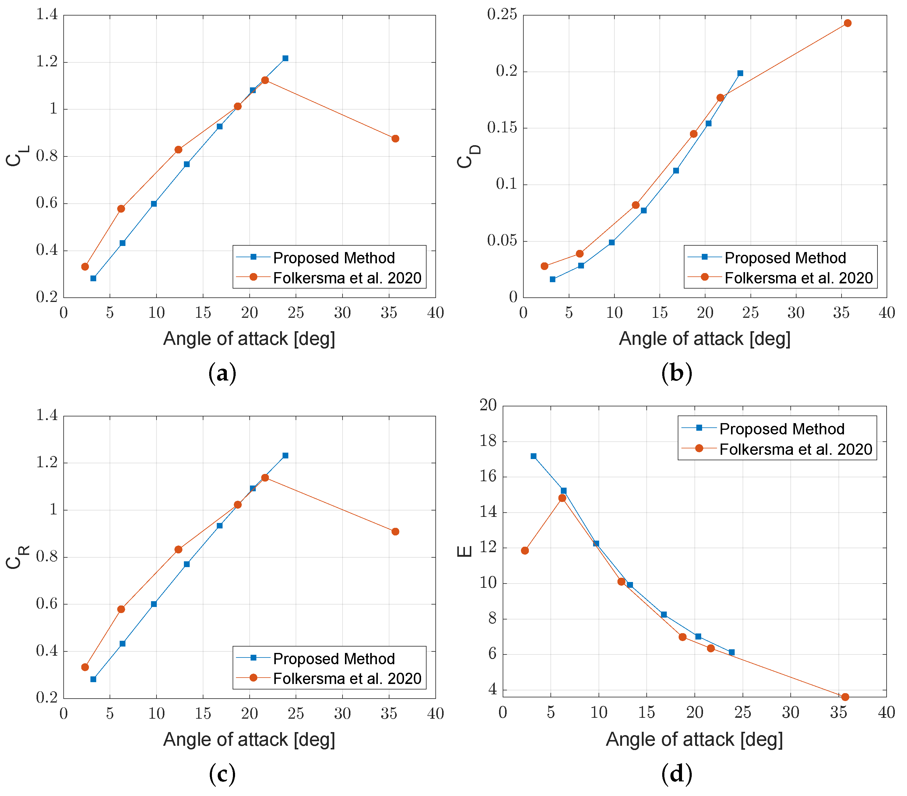
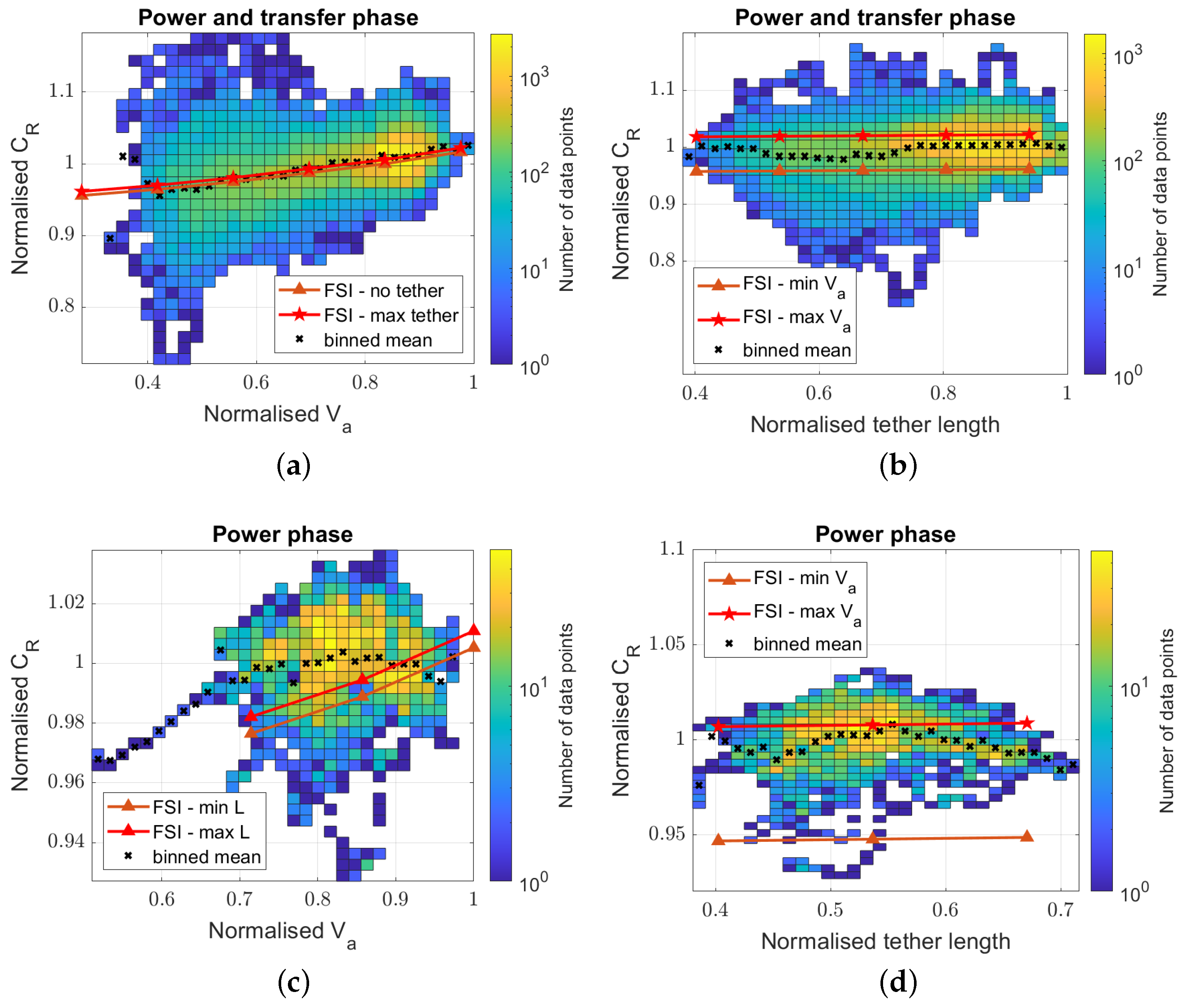
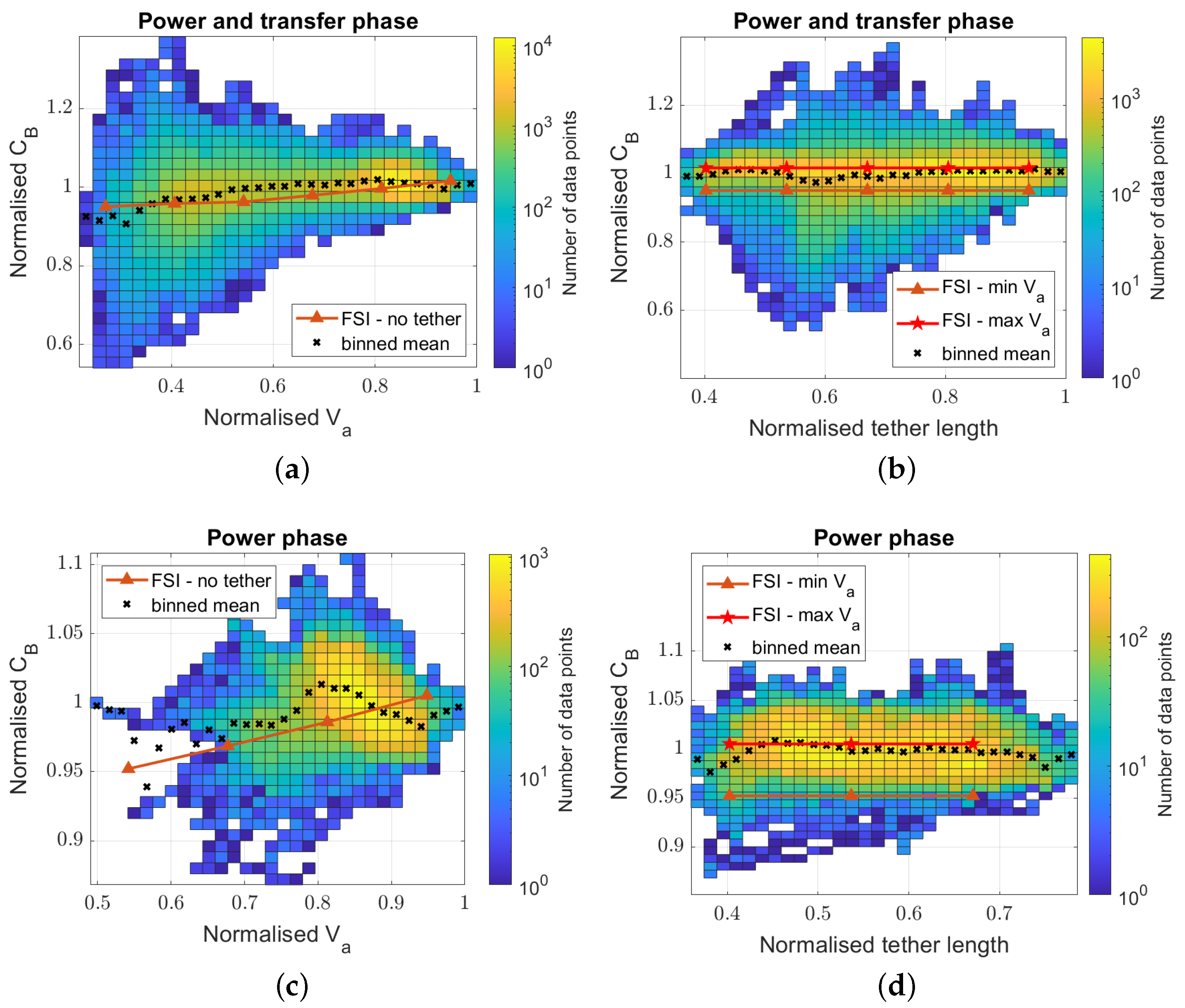
3.2. Tether and Belt Force Coefficients

Next, the computed tether and belt force coefficients were compared to the measurement data. The diagrams in this section depict the measured force coefficients as histograms, with each tile being colored according to the number of data points recorded for that specific range of the coefficient for a given range of apparent wind speed or tether length. Additionally, the binned mean of all tiles in a column is plotted as a black cross. The simulations were performed for a minimum tether length $L_{\mathrm{t}}$, with the tether completely reeled in, and a maximum length, where it was completely reeled out.

Figure 10a,b show the tether force coefficient $C_{\mathrm{R}}$ during the power and transfer phases.

It can be seen that the deviation from the mean is larger for the lower apparent wind speeds when the tether force is also lower and that the kite is more susceptible to gusts and other unsteady external factors. For larger values of $V_{\mathrm{a}}$, the data exhibit a maximum deviation of 15% from the mean and an overall positive slope of $C_{\mathrm{R}}$ with increasing $V_{\mathrm{a}}$. This positive slope highlights an interesting feature of the parafoil: an improved flight performance at higher aerodynamic loading. Possible reasons for this are an increase in the angle of attack due to deforming bridle lines, a change in rib profile, or a local change in the twist of the wing. The simulation results plotted in red approximately coincide with the mean of the data points and exhibit a positive slope. No significant deviation between the simulation results using no tether and the maximum tether length on $C_{\mathrm{R}}$ can be seen.

With this specific visualization technique, the data in Figure 10a show a good agreement between simulation and measurement, except for low values of $V_{\mathrm{a}}$. In Figure 10b, the resultant force coefficient is plotted against the tether length, and it can be seen that the binned mean values and the simulation results with maximum $V_{\mathrm{a}}$ fit well for tether lengths above 0.8. The force coefficient determined by the simulations appears to be slightly increased for longer tethers, following the binned mean values of the measurements, except for tether lengths below 0.6 where the measured coefficient is increases by almost 10%.

The resultant force coefficient was also compared to data recorded during the power phases only. Figure 10c depicts the resultant coefficient plotted against $V_{\mathrm{a}}$. and similar to the measurements including the transfer phases, the coefficient exhibits a positive slope for increasing $V_{\mathrm{a}}$. The simulation results underestimate the binned mean values by approximately 5%, where most data were recorded. Similarly, Figure 10d shows the coefficient plotted against the tether length, and the binned mean values display a slightly decreasing slope which is the opposite trend compared to the data including the transfer phases. The simulation results based on the maximum apparent wind speed slightly underestimate the binned mean values of the measurements.

Next, the belt force coefficient $C_{\mathrm{B}}$ was compared to the experimental data. Figure 11a,b displays the coefficient during power and transfer phases plotted against $V_{\mathrm{a}}$ and tether length, respectively.

The binned mean values of the measurements and the simulation results both exhibit a positive slope with increasing $V_{\mathrm{a}}$ and tether length. The simulation results lie within 5% of the binned mean, and the increasing trend for the force coefficient as a function of $V_{\mathrm{a}}$ is similar to the behavior of the tether force coefficient.

Figure 11c,d show the power phase only, and it can be seen that the density of the data points is lower but more concentrated around higher velocities. Again, the measured force coefficient and the simulation results show a good resemblance. It can be concluded that the simulation results correctly reflect the increasing trend of the force coefficients with increasing velocity. Moreover, the data measurements do not show a clear trend in force coefficients with varying tether lengths. The discrepancy between measured and simulated force coefficients lies within 5%, which is a good result for an initial design tool with an aerodynamic flow field obtained with potential flow theory. It should be noted that the spread in data points for various velocities and tether lengths clearly show that the test setup and measurement procedure suffer substantially from the unsteady wind field and kite–tether dynamics, as well as possible changes in the angle of attack.

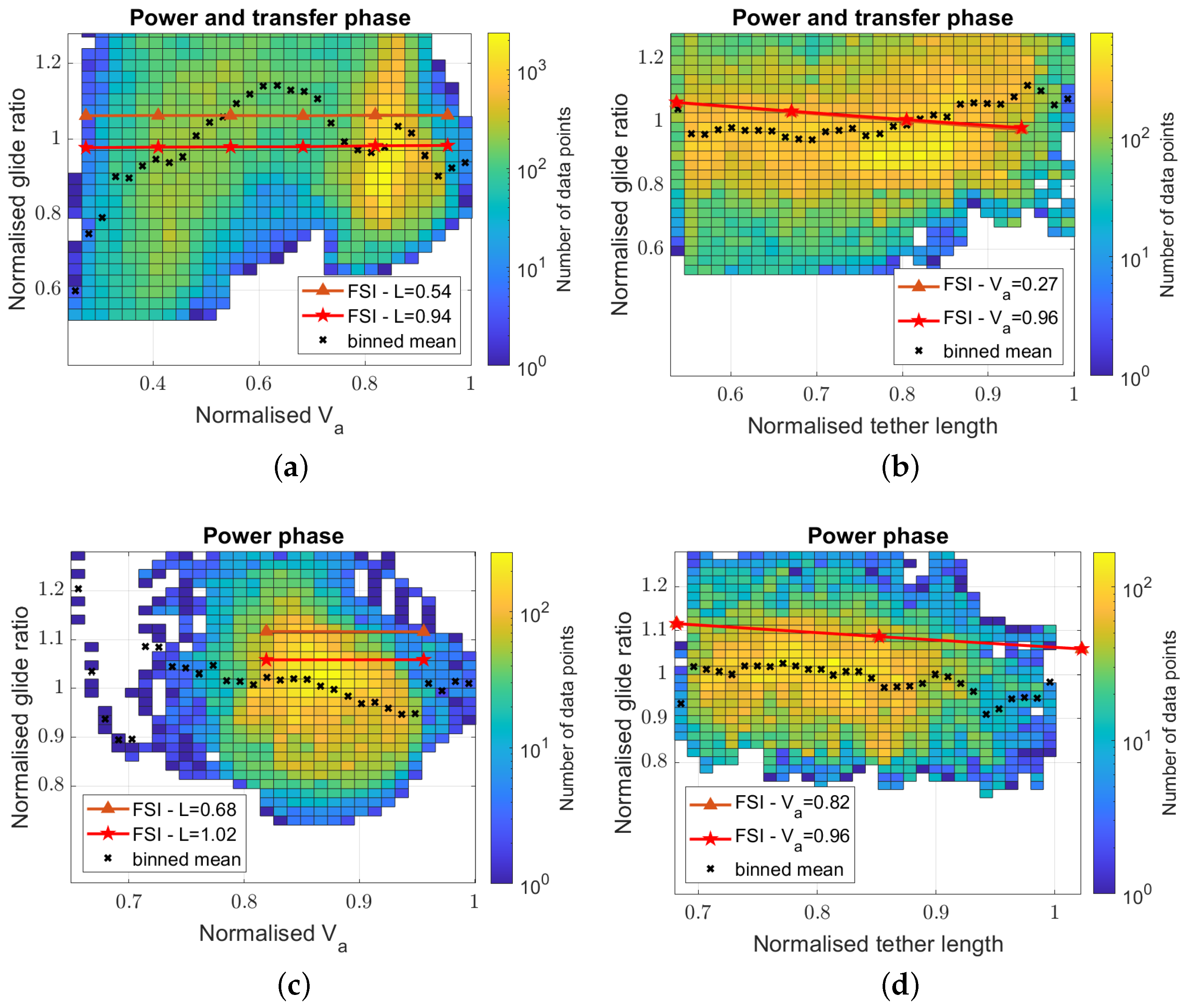
3.3. Glide Ratio

In this section, Equation (8) is used to determine the glide ratio of the airborne system from measurement data, which is then compared with simulation results. The same visualization technique as described in the previous section is used for the experimental data. Figure 12a,b depict histograms of measurement data recorded during both the power and transfer phases as a function of $V_{\mathrm{a}}$ and tether length, respectively.

The glide ratio given by the binned mean values fluctuates between 0.9 and 1.15 over the range of velocities, especially in the midrange, where the data are sparse, and the binned mean values should be interpreted with care. From this data, a clearly increasing or decreasing trend with $V_{\mathrm{a}}$ cannot be easily identified, mostly because of the large spread of the data. A similar picture can be seen in Figure 12b, where the binned glide ratio exhibits smaller fluctuations over the range of tether lengths, and a slight increase in glide ratio can be seen. This trend is opposite to the simulation results, which show a reduction in glide ratio for a longer tether, and considering the verification performed on the tether drag influence, this trend should be expected. For both graphs, the simulation results indicate an overestimation of the glide ratio by approximately 5–10%.

Figure 12c,d shows the glide ratio solely measured during the power phases, and a different behavior can be observed. In both figures, the glide ratio exhibits a negative trend for larger values. The difference between the binned mean and the simulation results varies between 5–12%. A general overestimation of the glide ratio is expected due to the potential flow assumption, which overestimates lift at higher angles of attack, as could be seen in the comparison study with CFD results [18]. Two factors possibly cause the large spread in glide ratio described in this section. The first source of error lies in Equation (8) from which the glide ratio is computed. The equations of motion in [30] assume a perfectly stretched tether without sag and dynamic interaction between wind, kite, and winch. Furthermore, the model is based on a force equilibrium assumption that is not satisfied in a nonuniform wind environment and with a winch accelerating the kite during flight. The second source of uncertainty includes the sensors used to determine the glide ratio. The LIDAR determines a wind speed average of over 1 min and acts as a low-pass filter. The tether angle at the ground station measures $\vartheta$ to a high degree of accuracy, but due to the long tether, a time lag between forces acting on the kite and the angle measured at the ground station can occur.

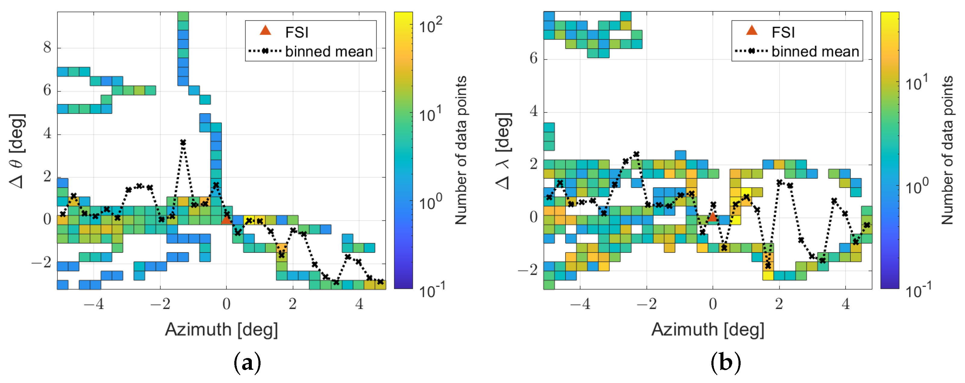
3.4. Neutral Flight

The final validation step was based on a neutral flight situation, during a time window of 5 min when the kite was positioned at a fixed downwind position at approximately a zero azimuth angle. The kite was controlled with small steering input to counteract wind gusts and turbulence to hold it in the same position. The simulation setup was similar to that described above: the symmetry boundary condition was kept at the center of the kite, and thus only half of the parafoil was modeled. Since the forces acting during a neutral flight are small compared to the power phases of the energy harvesting cycles, gravitational effects had to be taken into account in the simulation. Each component of the kite, such as the fabric, bridle lines, control pod, and the tether, were known masses, and the FE solver used these to include the distributed gravitational loading. For a kite in the neutral position, the apparent velocity is equivalent to the wind speed at flight altitude. Therefore, the measured LIDAR and ground wind speeds were taken as $V_{\mathrm{a}}$ at ground and flight altitudes, while the values in between were linearly interpolated. The converged result was then used to determine the elevation angle $\theta$ at the ground and $\lambda$ at the control pod, as depicted in Figure 13.

The most relevant measurements during the 5-min flight window are shown in Figure 14.

Both angular rates of the tether angles and the g-forces experienced by the control pod served as a selection procedure for the data to ensure a static flight. All data points with an angular rate deviation of 0.03 deg/s from zero and a g-force deviation larger than 0.01 were excluded. It can be seen in the tether angle $\varphi$ that the kite was drifting during the 5 min of flight, and for the validation, only data points between −5 and 5 degrees were considered. The tether angles $\vartheta$ and $\varphi$, as defined in Figure 2a, were measured with two rotary encoders, while the elevation angle at the control pod was derived from IMU data. The operator $\Delta$ quantified the difference between the simulation results and measured data.

Figure 15a,b depict this difference in the elevation angle at the ground and the control pod. It can be seen that the data are sparse due to the short flight window and data selection criterion. For the elevation angle at the ground, the difference between the simulation and measurement stays within ±1 degree, while for the control pod elevation angle, it is approximately within ±2 degrees. The simulation results of the kite-tether system show that the developed method can approximate both elevation angles to a satisfying degree of accuracy. The measured data also show how complex the interpretation of the kite system in a real wind environment is. In addition to fluctuations in the wind field, dynamic interactions between kite and tether create a time delay between measured accelerations at the kite and the ground station. Furthermore, despite the pilot’s effort to keep the kite aligned with the wind vector, the kite tended to drift slightly off, possibly due to changing wind direction at flight altitude.

4. Conclusions

A numerical method has been developed to determine the quasi-steady equilibrium shape and flight state of a ram-air kite during flight. The fluid–structure interaction problem was solved by computing the aerodynamic surface pressure distribution with the potential flow solver APAME and the shape deformation with the FEM solver mem4py, which were coupled via the library preCICE. The in-house-developed FEM solver is based on the kinetic dynamic relaxation method combined with a wrinkling model. The method was numerically stable and accurately found the equilibrium state of an inflated ram-air kite in a relatively short time. This is of particular importance at an early design stage when many different configurations have to be iterated and their aerodynamic performance and steering behavior assessed. Compared to analytical and numerical methods described in the literature, the developed FSI solver performed well even for large deformations of the membrane wing. The FSI solver was validated using measurement data from flight tests. The computed tether and steering belt force coefficients agreed well with the measured data for various flight speeds. The glide ratio was derived from the flight data and compared with the simulation results. It was found that the simulation overestimates the glide ratio by approximately 5–15%, depending on the flight speed. Moreover, the data showed a considerable spread of the glide ratio, which can be explained by the various assumptions required to derive the glide ratio from the measurements. A neutral flight situation was simulated accounting for both tether and gravitational effects. The computed elevation angles at the ground station and the control pod showed a satisfying accuracy within 1–2 degrees.

References

- International Renewable Energy Agency (IRENA). Renewable Power Remains Cost-Competitive amid Fossil Fuel Crisis. Available online: https://www.irena.org/News/pressreleases/2022/Jul/Renewable-Power-Remains-Cost-Competitive-amid-Fossil-Fuel-Crisis (accessed on 13 January 2023).
- Weber, J.; Marquis, M.; Cooperman, A.; Draxl, C.; Hammond, R.; Jonkman, J.; Lemke, A.; Lopez, A.; Mudafort, R.; Optis, M.; et al. Airborne Wind Energy. Technical Report NREL/TP-5000-79992, National Renewable Energy Laboratory (NREL). 2021. Available online: https://www.nrel.gov/docs/fy21osti/79992.pdf (accessed on 1 February 2022).
- Argatov, I.; Rautakorpi, P.; Silvennoinen, R. Estimation of the mechanical energy output of the kite wind generator. Renew. Energy 2009, 34, 1525–1532. [Google Scholar] [CrossRef]
- Luchsinger, R.H. Pumping Cycle Kite Power. In Airborne Wind Energy; Ahrens, U., Diehl, M., Schmehl, R., Eds.; Green Energy and Technology; Springer: Berlin/Heidelberg, Germany, 2013; Chapter 3; pp. 47–64. [Google Scholar] [CrossRef]
- Erhard, M.; Strauch, H. A Simple Comprehensible Model of Tethered Kite Dynamics. In Airborne Wind Energy; Ahrens, U., Diehl, M., Schmehl, R., Eds.; Green Energy and Technology; Springer: Berlin/Heidelberg, Germany, 2013; Chapter 8; pp. 141–165. [Google Scholar] [CrossRef]
- van der Vlugt, R.; Bley, A.; Schmehl, R.; Noom, M. Quasi-Steady Model of a Pumping Kite Power System. Renew. Energy 2019, 131, 83–99. [Google Scholar] [CrossRef]
- Cherubini, A.; Papini, A.; Vertechy, R.; Fontana, M. Airborne Wind Energy Systems: A review of the technologies. Renew. Sustain. Energy Rev. 2015, 51, 1461–1476. [Google Scholar] [CrossRef]
- Vermillion, C.; Cobb, M.; Fagiano, L.; Leuthold, R.; Diehl, M.; Smith, R.S.; Wood, T.A.; Rapp, S.; Schmehl, R.; Olinger, D.; et al. Electricity in the air: Insights from two decades of advanced control research and experimental flight testing of airborne wind energy systems. Annu. Rev. Control 2021, 52, 330–357. [Google Scholar] [CrossRef]
- Paulig, X.; Bungart, M.; Specht, B. Conceptual Design of Textile Kites Considering Overall System Performance. In Airborne Wind Energy; Ahrens, U., Diehl, M., Schmehl, R., Eds.; Springer: Berlin/Heidelberg, Germany, 2013; pp. 547–562. [Google Scholar] [CrossRef]
- Dunker, S. Ram-Air Wing Design Considerations for Airborne Wind Energy. In Airborne Wind Energy; Ahrens, U., Diehl, M., Schmehl, R., Eds.; Green Energy and Technology; Springer: Berlin/Heidelberg, Germany, 2013; pp. 517–546. [Google Scholar] [CrossRef]
- Desabrais, K.J.; Bergeron, K.; Nyren, D.; Johari, H. Aerodynamic investigations of a ram-air parachute canopy and an airdrop system. In Proceedings of the 23rd AIAA Aerodynamic Decelerator Systems Technology Conference, Daytona Beach, FL, USA, 30 March–2 April 2015; pp. 1–17. [Google Scholar] [CrossRef]
- Benedetti, D.M.; Veras, C.A.G. Wind-Tunnel Measurement of Differential Pressure on the Surface of a Dynamically Inflatable Wing Cell. Aerospace 2020, 8, 34. [Google Scholar] [CrossRef]
- Thedens, P.; Oliveira, G.; Schmehl, R. Ram-Air Kite Airfoil and Reinforcements Optimization for Airborne Wind Energy Applications. Wind Energy 2019, 22, 653–665. [Google Scholar] [CrossRef]
- Ortega, E.; Flores, R.; Pons-Prats, J. Ram-air parachute simulation with panel methods and staggered coupling. J. Aircr. 2017, 54, 807–814. [Google Scholar] [CrossRef]
- Fogell, N.A.T. Fluid-Structure Interaction Simulation of the Inflated Shape of Ram-Air Parachutes. Ph.D. Thesis, Imperial College London, London, UK, 2014. [Google Scholar] [CrossRef]
- Fogell, N.A.; Iannucci, L.; Bergeron, K. Fluid-structure interaction simulation study of a semi-rigid ram-air parachute model. In Proceedings of the 24th AIAA Aerodynamic Decelerator Systems Technology Conference, Denver, CO, USA, 5–9 June 2017; p. 3547. [Google Scholar] [CrossRef]
- Lolies, T.; Gourdain, N.; Charlotte, M.; Belloc, H.; Goldsmith, B. Numerical Methods for Efficient Fluid–Structure Interaction Simulations of Paragliders. Aerotec. Missili Spaz. 2019, 98, 221–229. [Google Scholar] [CrossRef]
- Folkersma, M.; Schmehl, R.; Viré, A. Steady-state aeroelasticity of a ram-air wing for airborne wind energy applications. J. Phys. Conf. Ser. 2020, 1618, 032018. [Google Scholar] [CrossRef]
- Thedens, P. mem4py Repository. Available online: https://github.com/pthedens/mem4py (accessed on 1 February 2023).
- Thedens, P. An Integrated Aero-Structural Model for Ram-Air Kite Simulations with Application to Airborne Wind Energy. Ph.D. Thesis, Delft University of Technology, Delft, The Netherlands, 2022. [Google Scholar] [CrossRef]
- Fagiano, L.; Quack, M.; Bauer, F.; Carnel, L.; Oland, E. Autonomous Airborne Wind Energy Systems: Accomplishments and Challenges. Annu. Rev. Control Robot. Auton. Syst. 2022, 5, 603–631. [Google Scholar] [CrossRef]
- Schmehl, R.; Noom, M.; van der Vlugt, R. Traction Power Generation with Tethered Wings. In Airborne Wind Energy; Ahrens, U., Diehl, M., Schmehl, R., Eds.; Green Energy and Technology; Springer: Berlin/Heidelberg, Germany, 2013; Chapter 2; pp. 23–45. [Google Scholar] [CrossRef]
- Dunker, S. Tether and Bridle Line Drag in Airborne Wind Energy Applications. In Airborne Wind Energy; Schmehl, R., Ed.; Green Energy and Technology; Springer: Singapore, 2018; pp. 29–56. [Google Scholar] [CrossRef]
- Filković, D. Apame—Aircraft 3D Panel Method. Available online: https://www.3dpanelmethod.com (accessed on 1 June 2022).
- Barnes, M.R. Form-finding and analysis of prestressed nets and membranes. Comput. Struct. 1988, 30, 685–695. [Google Scholar] [CrossRef]
- Barnes, M.R. Form finding and analysis of tension structures by dynamic relaxation. Int. J. Space Struct. 1999, 14, 89–104. [Google Scholar] [CrossRef]
- Jarasjarungkiat, A.; Wüchner, R.; Bletzinger, K.U. A wrinkling model based on material modification for isotropic and orthotropic membranes. Comput. Methods Appl. Mech. Eng. 2008, 197, 773–788. [Google Scholar] [CrossRef]
- Bungartz, H.J.; Lindner, F.; Gatzhammer, B.; Mehl, M.; Scheufele, K.; Shukaev, A.; Uekermann, B. preCICE—A fully parallel library for multi-physics surface coupling. Comput. Fluids 2016, 141, 250–258. [Google Scholar] [CrossRef]
- Oehler, J.; Schmehl, R. Aerodynamic Characterization of a Soft Kite by in Situ Flow Measurement. Wind. Energy Sci. 2019, 4, 1–21. [Google Scholar] [CrossRef]
- Erhard, M.; Strauch, H. Automatic Control of Pumping Cycles for the SkySails Prototype in Airborne Wind Energy. In Airborne Wind Energy: Advances in Technology Development and Research; Schmehl, R., Ed.; Springer: Singapore, 2018; pp. 189–213. [Google Scholar] [CrossRef]
Disclaimer/Publisher’s Note: The statements, opinions and data contained in all publications are solely those of the individual author(s) and contributor(s) and not of MDPI and/or the editor(s). MDPI and/or the editor(s) disclaim responsibility for any injury to people or property resulting from any ideas, methods, instructions or products referred to in the content. |
© 2023 by the authors. Licensee MDPI, Basel, Switzerland. This article is an open access article distributed under the terms and conditions of the Creative Commons Attribution (CC BY) license (https://creativecommons.org/licenses/by/4.0/).
Share and Cite
Thedens, P.; Schmehl, R. An Aero-Structural Model for Ram-Air Kite Simulations. Energies 2023, 16, 2603. https://doi.org/10.3390/en16062603
Thedens P, Schmehl R. An Aero-Structural Model for Ram-Air Kite Simulations. Energies. 2023; 16(6):2603. https://doi.org/10.3390/en16062603
Chicago/Turabian StyleThedens, Paul, and Roland Schmehl. 2023. "An Aero-Structural Model for Ram-Air Kite Simulations" Energies 16, no. 6: 2603. https://doi.org/10.3390/en16062603
APA StyleThedens, P., & Schmehl, R. (2023). An Aero-Structural Model for Ram-Air Kite Simulations. Energies, 16(6), 2603. https://doi.org/10.3390/en16062603