Article

Wind Power Forecasts and Network Learning Process Optimization through Input Data Set Selection

Faculty of Electrical Engineering, Automatics, Computer Science and Biomedical Engineering, AGH University of Science and Technology, 30-059 Krakow, Poland
*
Author to whom correspondence should be addressed.
Energies 2023, 16(6), 2562; https://doi.org/10.3390/en16062562
Submission received: 23 January 2023 / Revised: 18 February 2023 / Accepted: 21 February 2023 / Published: 8 March 2023

Abstract

:
Energy policies of the European Union, the United States, China, and many other countries are focused on the growth in the number of and output from renewable energy sources (RES). That is because RES has become increasingly more competitive when compared to conventional sources, such as coal, nuclear energy, oil, or gas. In addition, there is still a lot of untapped wind energy potential in Europe and worldwide. That is bound to result in continuous growth in the share of sources that demonstrate significant production variability in the overall energy mix, as they depend on the weather. To ensure efficient energy management, both its production and grid flow, it is necessary to employ forecasting models for renewable energy source-based power plants. That will allow us to estimate the production volume well in advance and take the necessary remedial actions. The article discusses in detail the development of forecasting models for RES, dedicated, among others, to wind power plants. Describes also the forecasting accuracy improvement process through the selection of the network structure and input data set, as well as presents the impact of weather factors and how much they affect the energy generated by the wind power plant. As a result of the research, the best structures of neural networks and data for individual objects were selected. Their diversity is due to the differences between the power plants in terms of location, installed capacity, energy conversion technology, land orography, the distance between turbines, and the available data set. The method proposed in the article, using data from several points and from different meteorological forecast providers, allowed us to reduce the forecast error of the NMAPE generation to 3.3%.

1. Introduction

The share of renewable energy sources in the energy mix in most European countries is rising steadily. The process is irreversible. That happens also because the cost of energy generated by RES is becoming more and more competitive against the prices of energy from conventional fuels, such as fossil fuels, gas, or nuclear energy [1]. Photovoltaic and wind sources take a special place among renewable energy sources on account of their potential and availability. For example, the energy potential of wind is estimated at 52 TW [2], and solar energy at over 1.94 TW [3]. Primary energy resources from those sources strongly depend on the existing weather conditions. That, combined with a growing share of renewable energy sources in the overall energy balance of countries/regions, forces energy producers and electric power system managers to collect increasingly more data, including, in particular, data on the current and predicted energy production from those sources.
There are two main factors that necessitate energy generation forecasting:
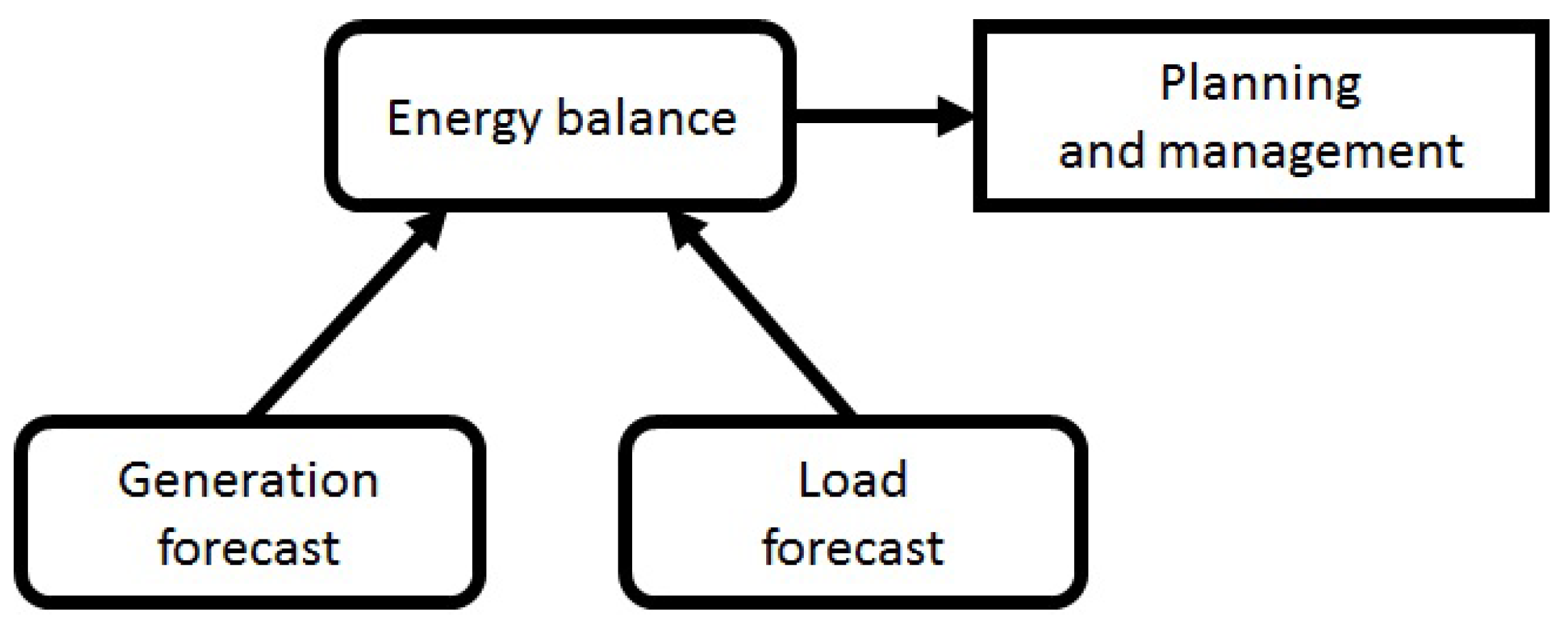
  • Energy balancing in the entire system, its selected area, region, energy community, etc., resulting from technical needs, e.g., to maintain system stability, to prevent overloading, to maintain the high quality of energy supply, to efficiently use energy and manage its flows in the supply networks, as well as from network development planning (Figure 1);
  • Electricity market, which has become a real-time market to an increasingly higher degree.
The proposed models for forecasting the electricity production of wind farms are the answer to problems in balancing the energy market from the day-ahead and intra-day perspectives. They make it possible to forecast energy production based on meteorological conditions, and thus allow the accuracy of the forecasting models of energy prices described in [4,5,6,7] to increase. The authors [4] emphasize the stochastic nature of wind farm production and their negative impact on the predictability of energy prices on the market. In an article [6] on the management of the multi-energy microgrids market, they consider five cases where the variability of wind farm production is predicted based on wind speed recording. Similarly, in [7], it is the only factor determining the amount of energy produced from wind farms. The analysis of the impact of weather factors carried out in this article, and the proposed method may have a positive impact on improving the credibility of microgrid and energy price management models. Quickly developing IT technologies allow the implementation of forecasting models that are complex in computational terms. They help to minimize forecasting errors to an increasing extent, thus enabling effective optimization of the load distribution and energy outflows, increasing energy supply security, and reducing the cost of its production and transmission. In addition, the adverse impact of the energy sector on the natural environment is reduced. A quick development of energy production volume forecasting can also be observed for wind power plants, which are the focus of the discussion in this paper. This area is being actively developed by research units from across the world. That is demonstrated by numerous papers devoted to this topic published by first-rate publishing houses [8,9,10,11,12,13,14,15,16]. The forecasting models they describe can be broken down into [16]:
  • Physical models (e.g., [17,18]).
  • Statistical models.
    -
    Based on data sets:
    *
    Naive models (persistence method) (e.g., [19]);
    *
    Grey forecasting models (e.g., [20]);
    *
    Models based on Kalman filters (e.g., [21]);
    *
    ARMA (Autoregressive moving average model) (e.g., [22]);
    *
    ARIMA (Autoregressive moving average model) (e.g., [19,23,24]).
    -
    Based on “artificial intelligence”:
    *
    Artificial neural networks (e.g., [25,26,27]);
    *
    Vector machines (e.g., [28]);
    *
    Wavelet analysis (e.g., [29,30]).
  • Hybrid models (being a combination of the above) (e.g., [26,29,31]).
Below in this paper, a review of the energy production forecasting methods is provided, with a particular focus on those that represent an alternative to the neural networks proposed in this article or methods employing neural networks in hybrid configurations. Those solutions have many proponents, but also opponents, who argue that the method uses fuzzy definitions, and hence its results are ambiguous and imprecise. It was long believed that they were not suitable for multi-stage computations (i.e., when the results of the first stage are inputs in the next one) [32]; however, deep learning networks come in handy here. Many years ago already, George Box, a British statistician dealing with quality control, analysis of time series, and Bayesian inference, noticed and accordingly titled one of the chapters in their paper [33], namely, “All models are wrong, but some are useful”. It is emphasized in the article that it is a very difficult task to map reality with a simple model. Linear models are well known and described by mathematicians, but they disappointingly rarely accurately reflect reality. Non-linear problems that are closer to reality are more difficult to define and solve. In those cases, artificial intelligence-based models come in handy, and even though they are unable to provide accurate solutions, owing to the proper definition of the attributes of the identified facilities, they can find relations that a given phenomenon shares and provide a solution to the problem with satisfactory accuracy.
Many statistical models can be distinguished, e.g., WPPT, FUGS, and other models described below. They were selected on account of a different approach to the data processing and forecasting process. Authors of the papers referred to above proposed their own forecasting methods based on individual input and verification data sets. The WPPT (Wind Power Prediction Tool) model [34] allows the forecasting of energy for a time horizon of up to 48 h, and a resolution of 30 min. Numerical weather forecasts are used for the forecasting, as well as wind farm measurement data updated on an ongoing basis, which can update the non-linear model on a continuous basis. The model combines two approaches by forecasting the output of the individual turbines within the farm and the output of the entire wind farm.
The FUGS (Forecasting Using Gaussian Processes) model [14] is dedicated to short-term (h-24 h) forecasting of wind energy production. It comprises two models: GP-CSpeed and GP-Direct. GP-Direct is built on data coming directly from numerical weather forecasts (without their additional adjustment). The second model, named GP-CSpeed, first adjusts the input data, and then the model itself is built on the basis of already adjusted values. Wind velocity adjustment involves filtering out the set of data that goes beyond the permitted limits. The same forecasting model is used in both cases.
The SVM (Support Vector Machine) [15] is an effective statistical tool that can solve multi-parameter non-linear problems. SVMs are learning machines based on support vectors. An important advantage of the SVM network in comparison to MLP (Multilayer Perceptron) neural networks is turning the problem into a task that typically has a single minimum of the purpose function. A disadvantage of such solutions is the dependence of the results on the adopted values of constant parameters, such as the width of Gaussian function σ , factor γ for a multinominal core, the constant regularization value C (reducing network complexity), or tolerance ε [35].
The topics of network load and generation forecasting are very similar and do not differ in terms of the structure of the applied model. Paper [36] describes topics relating to the load forecasting of a specific part of the power supply system, being the effect of energy consumption and generation, paying particular attention to the challenge of RES generation forecasting. Paper [37] presents the options for load forecasting using the hybrid method based on artificial neural networks and using Mixed Integer Linear Programming techniques. In the latter method, the models that use historical and current electrical and forecasting data, combined with weather forecasts, are capable of effectively forecasting the system load. As noted by the authors, hybrid models that employ artificial neural networks and linear algorithms are mutually complementary, ensuring redundancy. The forecasts are generated by linear algorithms, whereas the neural network “fine-tune” the forecasts. That enables the incorporation of non-linearity of the predicted load and allows the achievement of significant accuracies.
To improve the forecasting accuracy, hybrid models are used that combine the advantages of both model types. A practical example of a hybrid forecasting model is described in paper [8]. A model presented there is dedicated to the energy production prediction for fourteen wind farms. The proposed hybrid model, combining neural networks and vector machines, was compared with other models based on either neural networks or vector machines only. Paper [8] describes ANN (Artificial Neural Networks) learning on the basis of historical data covering one year. The model considers wind velocity and direction as parameters underpinning the volume of energy production. A simple neural network was proposed, consisting of a single hidden layer, because adding new layers did not improve the results. There were from 15 to 25 neurons in the hidden layer, depending on the wind farm for which the forecasts are made. It follows from the observation of the authors of [8] that the qualitatively worst forecasts covered the power plants located in rough terrain.
In the hybrid model [29], the data were divided into four intervals on the basis of IEWT (improved empirical wavelet transform), and then processed by a network of carrier vectors using the LS-SVM (least-squares support vector machines) method to find its parameters. The least-squares method (LS) is a tool that enables the minimization of the average-square error in the course of the determination of linear regression or estimation of non-linear model parameters [35]. At the same time, the BSA (Bird Swarm Algorithm) was used to achieve more precise forecasts [38]. As noted by the authors, that algorithm ensures better forecast accuracy relative to other models based on biological systems, such as differential evolution (DE), Genetic Algorithm (GA), and Particle Swarm Optimization (PSO). The application of BSA was used to select LS-SVM network parameters, which, as reported by the authors, markedly reduced the complexity of computations and improved forecasting accuracy.
An example of a neural network-based hybrid model with regressive error propagation is described in paper [39]. The authors of the paper effectively used that type of network in combination with NARX (Non-linear Autoregressive with External Input). NARX network models perform better with short-term forecasts, whereas network-based models with regressive error propagation ensure better results for longer forecasting horizons. The following was used for the forecasting: real-time production, structural information, NWP (Numerical Weather Prediction), and power forecast from various providers.
Many articles have been published referring to the prediction of energy production from wind farms using NWP data for forecasting. Unfortunately, these models are also burdened with an error, which can be minimized with the knowledge of the specificity of the operation of the wind farm. The authors [40] propose the use of additional data streams for forecasting. In addition to the classic Deterministic weather research and forecasting (WRFD), they also use Radar weather research and forecasting (RWRF) to reduce the horizontal resolution grid to 2 km. Increasing the amount of data allowed them to obtain better predictions; in most cases the MAPE error was below 8%. Promising results were obtained for the XGBoost (Extreme gradient boosting) and ANN models. In this case, only the wind speed was used for the forecasts, which seems to be a weakness of the models. In paper [41], long-term data from 2009 to 2011 were used to train the model. Wind direction was taken into account as an additional factor. Data from 12 points of the NWP forecasting grid were used to improve forecasts. Model verification was performed only for data from two months. For forecasting, support vector regression (SVR) was used, extended with stacked-denoising-autoencoder (SDAE) and bat algorithm (BA) optimization. The reduction in the NRMSE error to 11.6% is visible for the three hidden layers of the SDAE model. Larger errors were obtained for a smaller and larger number of layers (with one, two, four, or five hidden layers), which may indicate the need to select the appropriate number of layers. The combination of the SDAE-SVR-BA model allowed for a 1–2% increase in accuracy. The authors of [42] proposed alternative models being combining wave division (WD), improved gray wolf optimizer based on fuzzy C-means clusters (IGFCM), and Seq2Seq model with an attention mechanism based on the long short-term memory model (LSTMS). The advantage of LSTMS models is that they have feedback in their structure. As a result of the analysis, two models were selected for which the NMAE and NRMSE errors were the smallest in a one-day perspective. The first is the IGFCM-LSTMS model (Seq2Seq model with IGFCM) and the second is its modification WD-IGFCM-LSTMS that takes into account the wave division. The models generated forecasts with an NMAE error of 10.28–10.32% for Wind Farm A and 9.53–10.18% for Wind Farm B. Additional input data streams to the model are included in the paper [43]. Data from three NWP suppliers and many points located in the vicinity of the power plant were used. The power plant consisted of 68 wind turbines. As a result of combining data streams in the MIX model, it was possible to reduce the NMAE error of the wind speed forecast from 6.7 to 8% to 6.1% and the wind power forecast to 6.91%. The authors of the article confirm the benefit of using data from different providers of NWP models. In [44], the LSTM model with the modification of wind power ramp events (WPREs) was proposed. The method was tested for three wind farms. As a result of the prediction, the NMAPE error was obtained in the range of 9.4–15% (depending on the tested object). As the authors emphasize, better results were obtained using the WPRE functionality. The model better identifies changes in the type of ramp events, which has increased its accuracy. The authors of [45] used alternative machine learning methods such as support vector regression (SVR), random forests, and artificial neural networks to forecast farm power. Data with hourly resolution were used, such as wind speed at 10 and 80 m above sea level. As the authors emphasize, in most cases, the highest accuracy was obtained for classic artificial neural networks. Only for one power plant was the SVR method better.
Artificial neural networks were selected for this study because this method
  • is easy to implement, verify and improve;
  • enables the development of models for various objects, as presented in this article;
  • allows the use of data of various natures (meteorological, electrical);
  • makes it relatively easy to take into account additional factors affecting the amount of energy produced;
  • enables the continuous learning of the neural network. As a result, the quality of the forecast improves over time.
The purpose of this paper is to present new short-term (24 h) models for wind power plant generation forecasting. Forecast sensitivity to the specific weather factors (Section 2.2 and Section 2.3) was tested on the basis of actual measurements performed at four wind farms (Section 2.1). The analysis allowed us to select the most advantageous input data set structures and improve forecasting accuracy. The forecasting models proposed in this paper (Section 2.4) are a combination of the statistical model using artificial neural networks based on numerical weather forecasts. To improve the forecasting effectiveness, a few versions of the model were proposed and subsequently tested.

2. Data Set and Methods

The basic object for which energy production forecasts are performed is a single wind turbine. Forecasting for the entire farm, comprising many turbines, is more complex. In that case, additional factors should be considered, such as the number of currently working turbines, or terrain shape around each turbine comprising the wind farm. A change in wind velocity close to the turbine activation threshold may result in deactivation of some. Start-up is time-consuming, which affects the volume of the actual production and forecasting error.
On the basis of data from 4 wind farms, factors that impact the energy production value were analyzed, and sensitivity analysis was performed. Only such data were selected for the analysis that can be monitored for a given object, and which can be potentially significant for the forecasting. The descriptions of the respective facilities are heterogeneous due to a different set of recorded values and available information. The collected database and analysis performed on its basis seeks to simplify, in the future, the process of developing forecasting models for new facilities.
In the case of the proposed forecasting methods that are based on artificial intelligence, data from the power plant provide information about key factors influencing its operation.

2.1. Analyzed Wind Power Plants

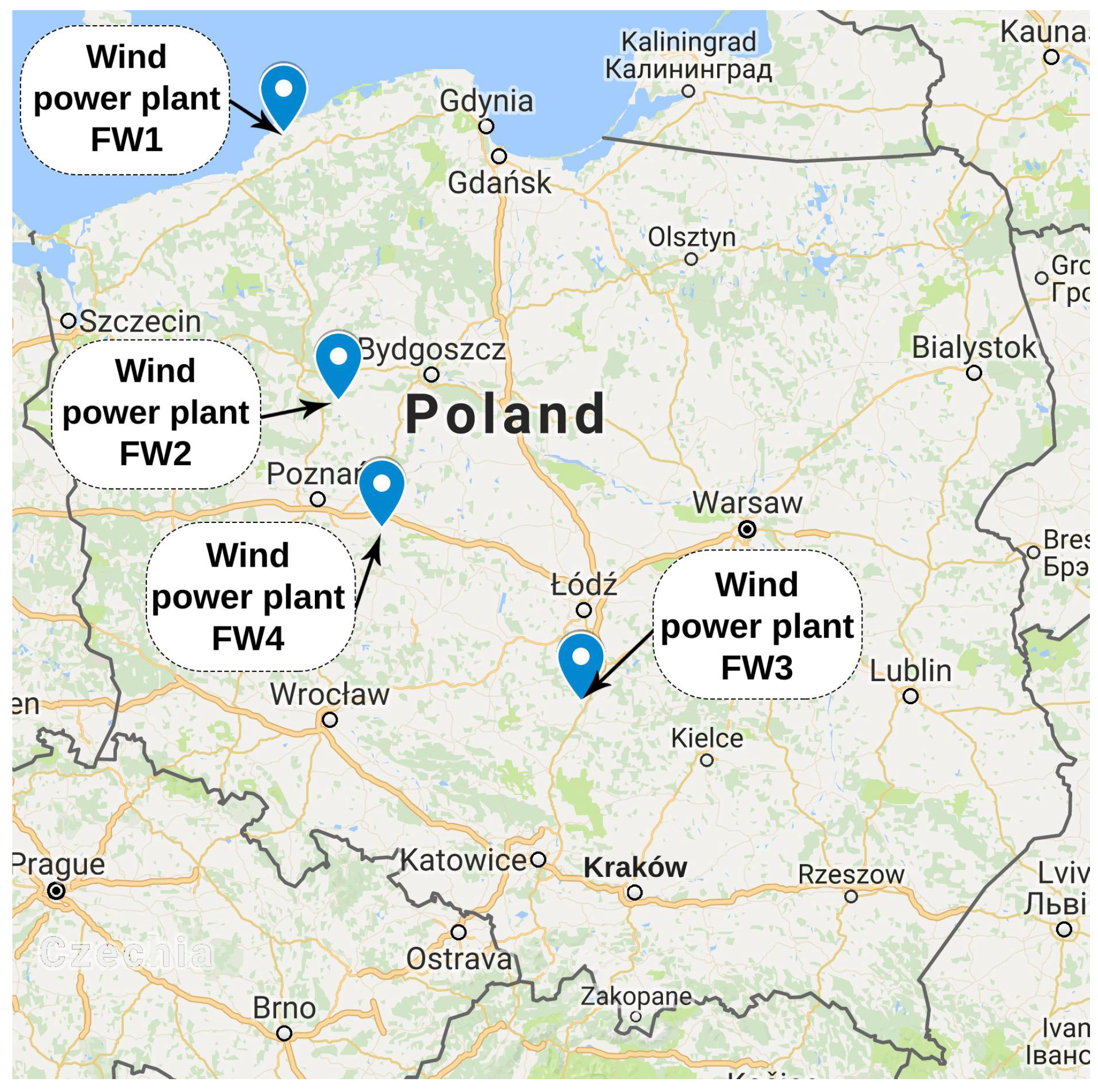
Figure 2 shows the location of the contemplated power plants on the map of Poland.
Data come from the following facilities:
  • Wind power plant No. 1 (FW1), located in the central area of the Baltic Sea coast, whose total installed capacity of wind turbine units equals 8 × 2.5 [MW];
  • Wind power plant No. 2 (FW2), located in northwestern part of the country, whose total installed capacity of wind turbine units equals 60 × 2.0 [MW];
  • Wind power plant No. 3 (FW3), located in south-central part of the country, whose total installed capacity of wind turbine units equals 15 × 2.0 [MW];
  • Wind power plant No. 4 (FW4), located in central-western part of the country, whose total installed capacity equals 1.0 [MW], comprises a single turbine, and therefore, local wind variability directly affects changes in the generating unit’s output. That hinders the forecasting process, and therefore, it was decided to include it in the analysis.
Facilities were selected so that conclusions and results of the analysis could enable a proposal for a universal model that is scalable for other wind power plants located in the country.
The facilities identified above were selected on account of their variability in terms of the following:
  • Number and unit output of the turbines;
  • Location;
  • Type of generators/gears;
  • Elevation of the hub’s axis;
  • Rotor’s revolving surface area.

2.2. Dependence of Output on Wind Velocity

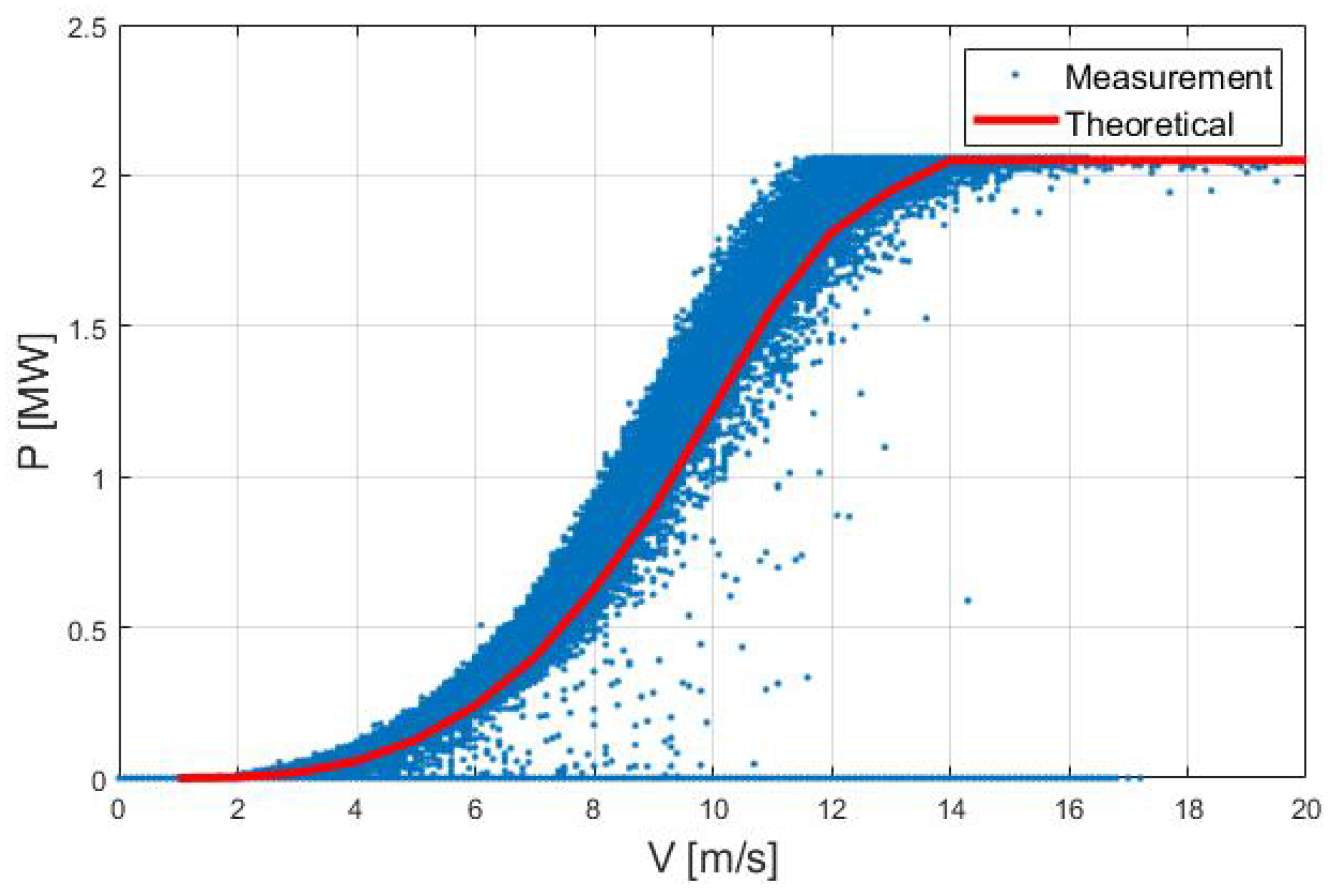
Figure 3 presents the declared power characteristics of an example wind turbine of power plant FW3 prepared on the basis of the manufacturer’s documentation [46] and as-measured historical data.
When analyzing Figure 3, the following can be identified:
  • The theoretical power characteristics are within the area demarcated by the measurements. That is because the wind turbine operates under variable weather conditions, different than those adopted when the theoretical power characteristics were developed;
  • There is a set of points on the actual power characteristic for the wind velocity from 4 [m/s] to 17 [m/s] for which power P = 0. This may be caused by an emergency or operating shutdown of the turbine, for example, if the wind velocity is too high, or due to icing or maintenance.
The wind velocity distribution within the wind farm, even though it is located in a relatively small area (270 ha), is not even. This is shown by Figure 4, presenting the annual deviation from the average electricity production for the respective turbines E1–E15 comprising wind power plant FW3.
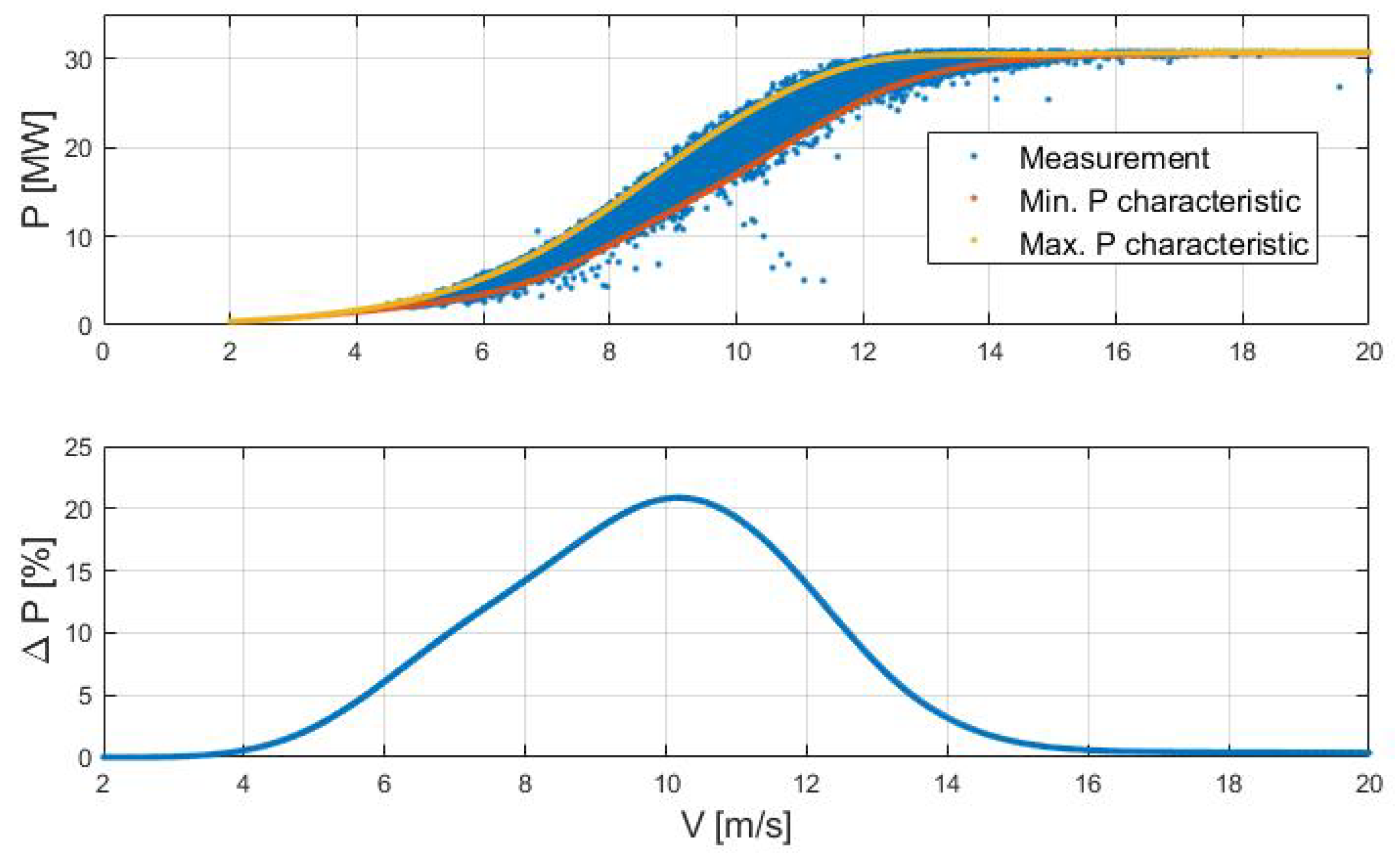
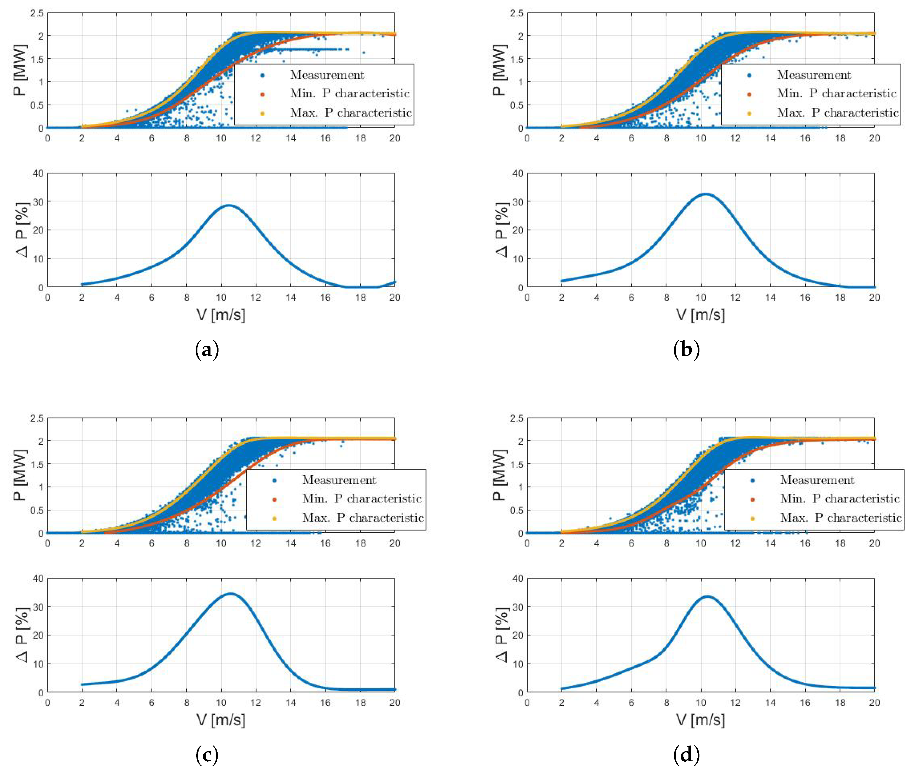
Figure 5 presents wind power plant output variability as a function of wind velocity value. The subsequent figures present similar characteristics for the selected turbines within power plant FW3 (Figure 6).
The volume of electricity production from wind power plants depends on many factors relating to both the construction and the type of generation, as well as the interconnected power equipment. Of significance are also weather factors, marked by strong variability and largely independent of humans. As time passes, power plant parameters are also subject to change as a result of the equipment aging process and reduced efficiency, which impacts the volume of energy production by the power plant.

2.3. Impact of Weather Factors on the Wind Power Plant Operation

The volume of electricity generated by the wind power plant strongly depends on weather factors, or the locations of the respective turbines within the farm. In the first case, it follows from the laws of physics governing the turbine’s operation, and in the second, from the shape of the terrain and mutual impact of the turbines, the so-called “overshadowing”. Wind power plants are typically located over a large area, and in effect, wind velocity distribution is uneven.
Wind velocity clearly has the largest impact on the volume of energy generation, but other impact factors were also analyzed, such as temperature, pressure, and wind direction.

2.3.1. Impact of Ambient Temperature on the Wind Power Plant Operation

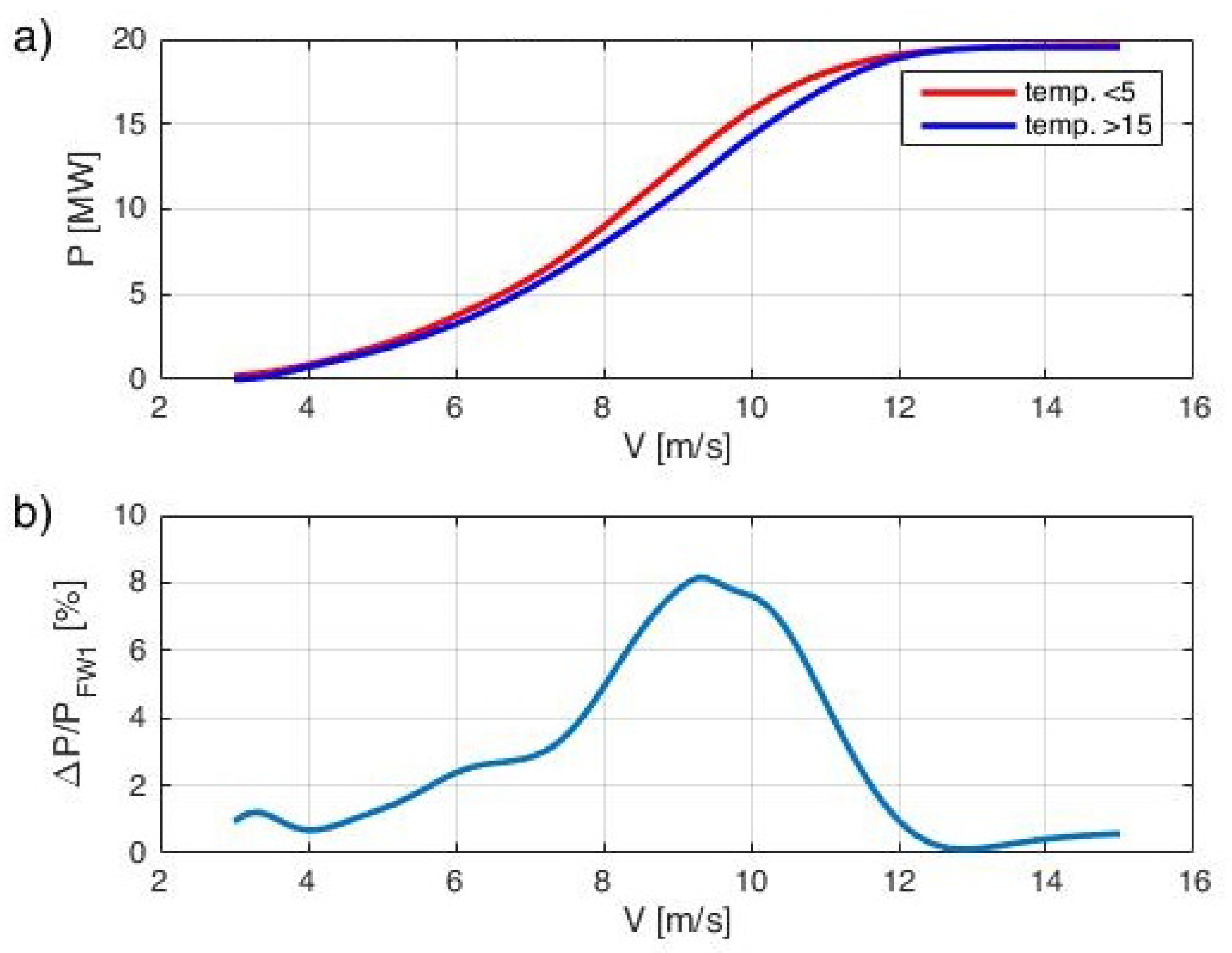
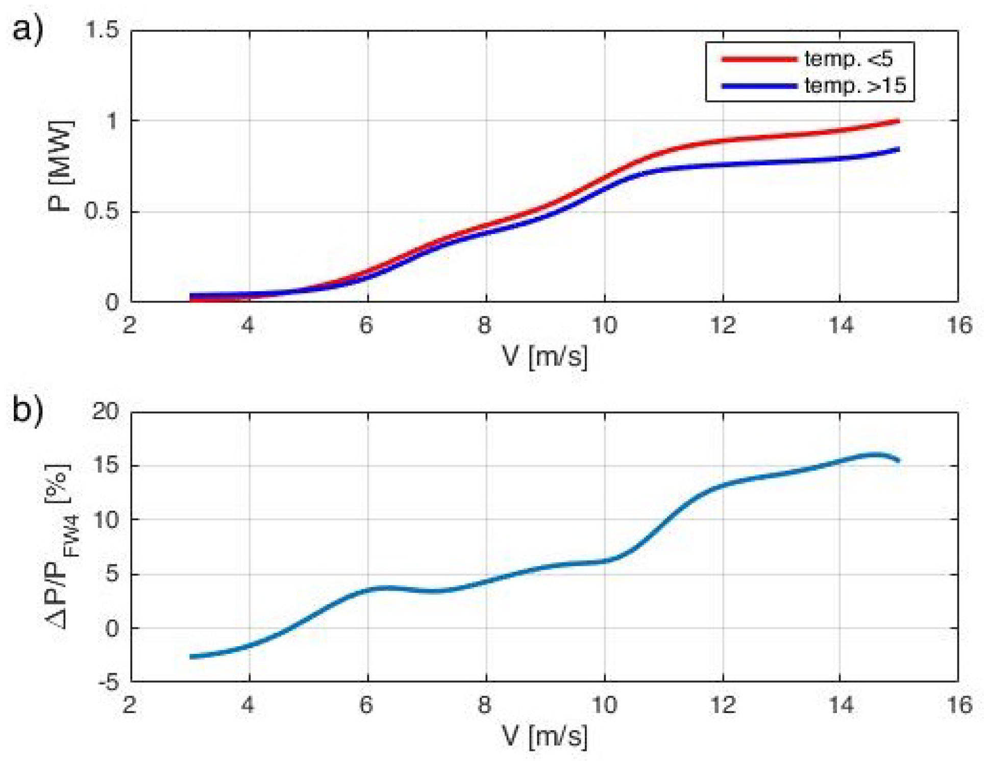
The analysis of the temperature impact, on account of the collected data set, was performed for wind power plants FW1, FW3, and FW4. The source data set is, in each case, divided into two subsets. One comprises data related to ambient temperature T < 5 C, and the other for temperature T > 15 C. The selection of the ranges was arbitrary, so that the adopted temperature limit values enabled reconstruction of the wind power plant power characteristics, meaning that sufficient quantity of data was present in the respective subsets. Temperature in the set was changing in the range from −17 C to 39 C. The selection of limit temperatures allowed us to obtain sets in a duplicated number (relative to the temperatures). Neural network models were developed for the two data sets received (for each power plant) (Figure 7).
Two prepared data sets (set A—T < 5 C, set B—T > 15 C) were used in the process of organizing the learning set and in the process of network learning. Wind velocity V and power P were provided for the neural network input and output.
After the end of the optimization process within the meaning of the medium-square error minimization, networks were obtained that allowed us to reconstruct the wind power plant characteristic P = f(V) for the highlighted subsets.
In both cases, the learning covered the neural network of identical typology. In the first two layers, the network comprised five neurons in each layer with a logistics activation function, and a single linear neuron in the output layer. The results of the wind power plant power curve reconstruction by the network are shown in Figure 8, Figure 9 and Figure 10.
Figure 8 shows two power characteristics, which are the neural network’s response to low (T < 5 C) and high temperatures (T > 15 C).
Figure 9 and Figure 10 include, as in the previous case, two power characteristics for power plants FW3 and FW4, respectively,
It follows from Figure 8 to Figure 10 that temperature affects the shape of the wind power plant power characteristic. In the case of wind power plant FW3, the largest difference is for the wind velocity of 9.4 m/s and is equal to 1.63 MW. That represents over 8% of the wind power plant’s rated output. The differences for wind power plants FW1 and FW4 grow bigger as the wind velocity increases, reaching as much as 10–15% of the power plant’s rated output.

2.3.2. Impact of Atmospheric Pressure on the Power Plant Operation

The impact of atmospheric pressure was analyzed in the same way as for the temperature. On account of the data in stock, the analysis was performed for one wind farm, FW1. Two data sets were separated. One included data for pressure lower than 997 hPa, and the other data for pressure that is greater than 1018 hPa. The selection of limit pressures was organized so that to obtain sets with a similar size, enabling reconstruction of the power characteristic. Neural network models were developed for the two data sets received (Figure 7). Neural models were proposed having the same structure as for the analysis of the impact of the ambient temperature on wind power plant operation, reconstructing the wind power plant’s power characteristic. Results of network learning are shown in Figure 11.
Pressure and power correlation coefficient for the wind power plant equals −0.24, which may testify to this factor having two times the impact of temperature. In reality, the impact may not be that significant due to proportionately small pressure changes over the year (pressure varied from 982 to 1035 hPa). Average pressure in the analyzed period of nearly two years was 1012 hPa, which, considering the difference between the highest and lower pressure being 53 hPa, gives the value changes equal to only 5% of the average. The results shown do not confirm significant impact of atmospheric pressure on the power characteristic curve of wind farm FW1.

2.3.3. Impact of Wind Direction on the Wind Farm Operation

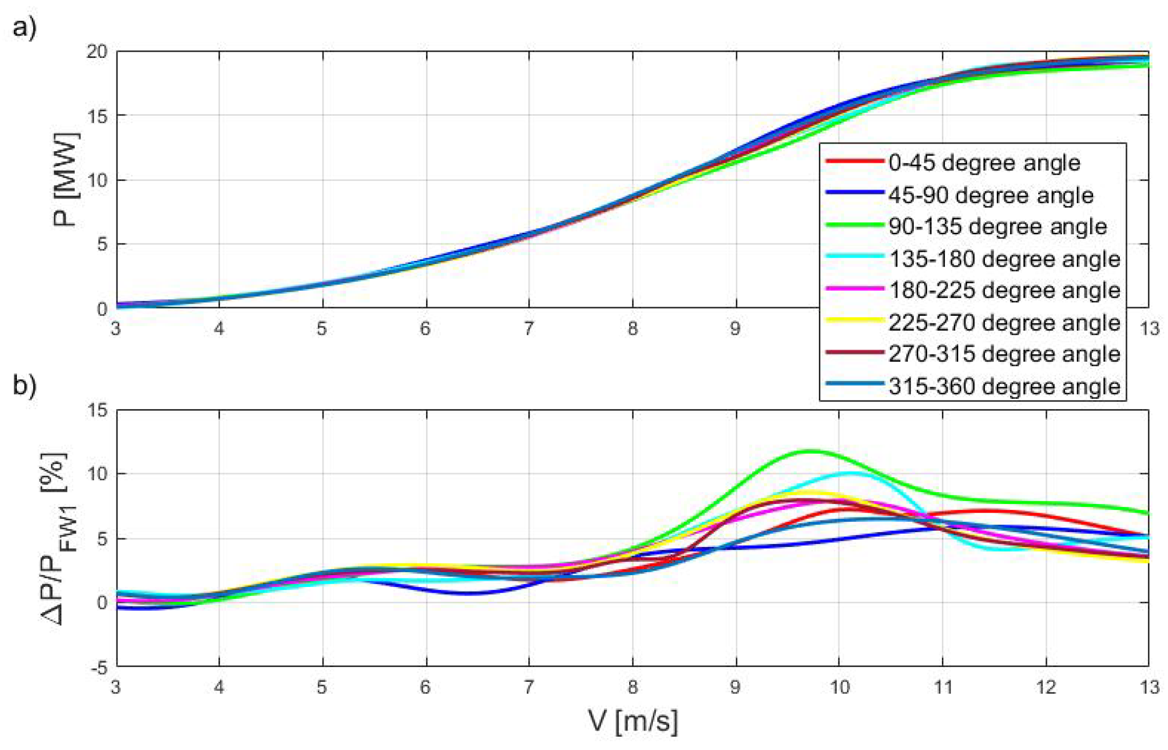
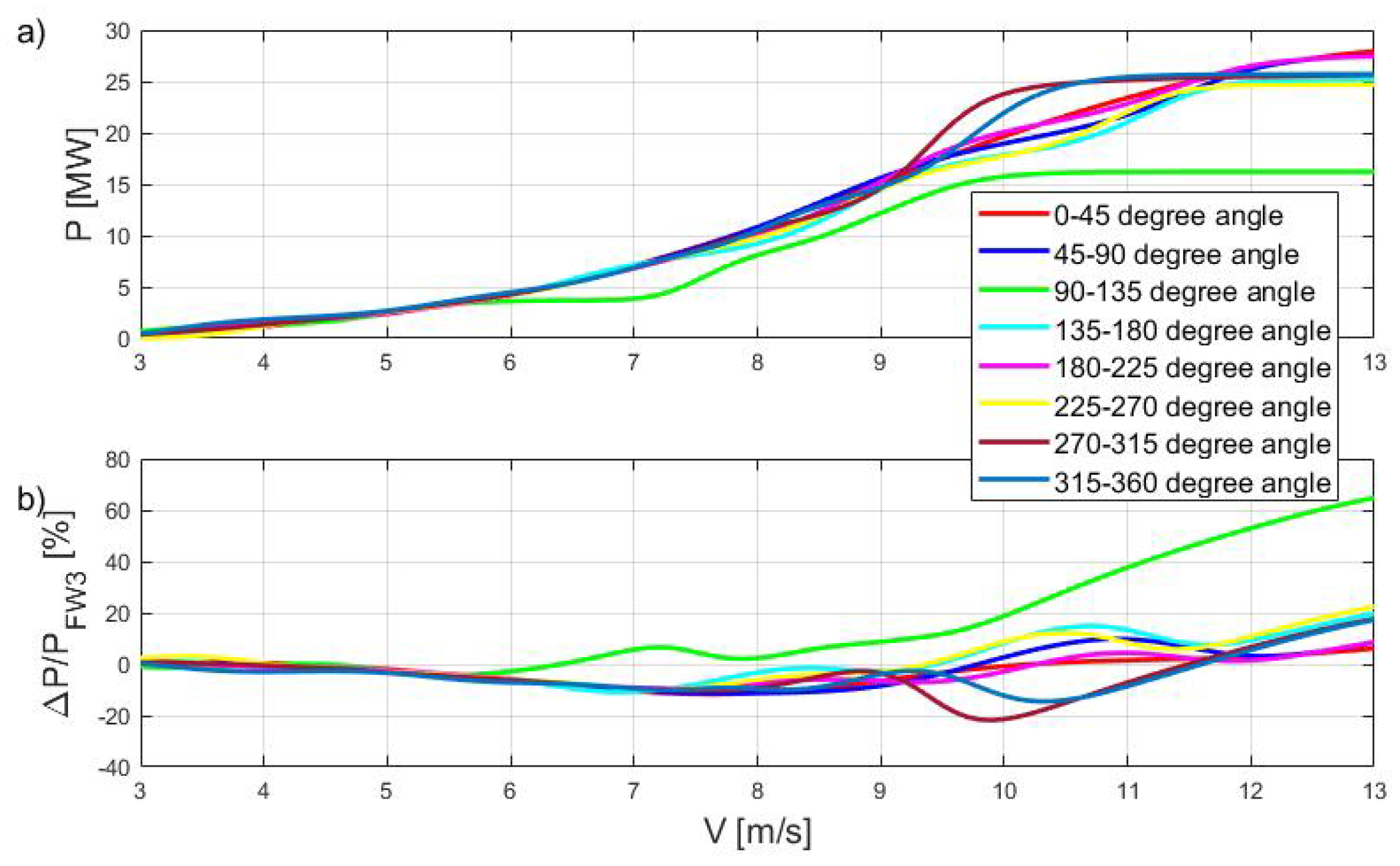
Eight data sets were selected, where the wind direction changed every 45 . The analysis was performed for the cases discussed above. Network learning results for wind farms FW1 and FW3 are shown in Figure 12 and Figure 13.
In analyzing the charts from Figure 12, one can notice that the differences in the velocity range from 3 to 8 m/s are insignificant, not exceeding 0.5 MW. At higher velocities, they grow to over 1 MW. There are slightly greater differences for wind power plant FW3 (Figure 13). However, this may be caused by the learning set being too small for the selected directions, which prevented the achievement of the full range of wind velocity and power variability (for power characteristic-building purposes).
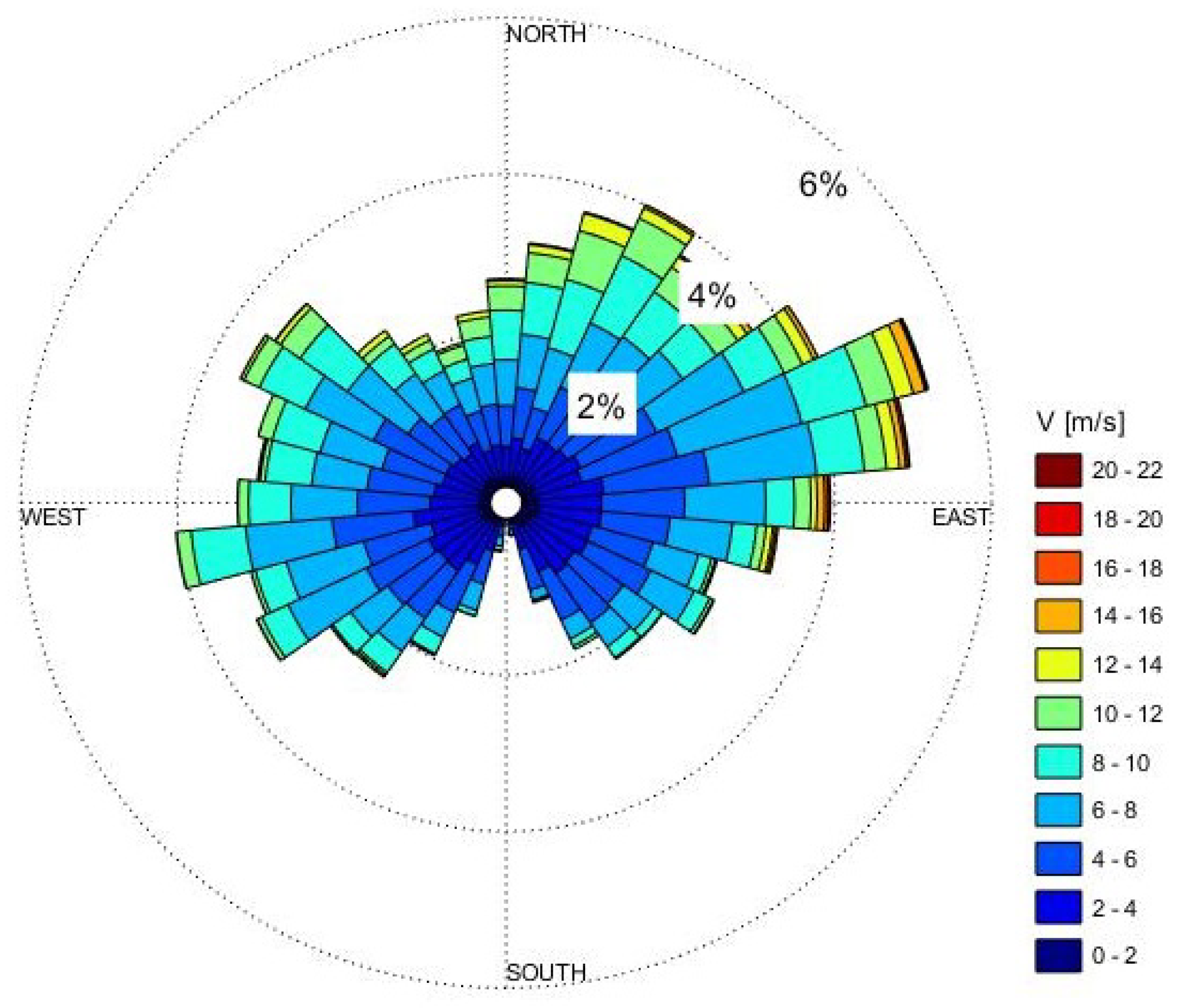
Figure 14 shows that the dominant directions are northern and northwestern, and the wind velocity variability for the remaining directions is small.
It is difficult to differentiate a trend in the analyzed data set that would indicate that wind direction impacts the power characteristic curves. The curves intertwine in the entire selected range, and no single or outlier curve can be singled out.
Similar information is supplied by the correlation table, where the factors for wind direction are 0.05–0.14. Table 1 shows the factors broken down into the respective wind directions. The correlation coefficient for wind direction and velocity broken down into 8 angular ranges varies from −0.19 to 0.1, which may show that there is no correlation between those parameters.
The volume of wind farm energy production strongly depends on whether factors variable over time that exist in the power plant’s immediate vicinity. The more precise the estimation of the value, the less expensive its balancing in the power system. However, these are not the only factors that affect energy production by those plants.

2.3.4. Summary of the Impact of Weather Factors

Table 2 presents the Pearson correlation coefficient among the analyzed factors in relation to the power plant’s output.
The strongest correlation is for the wind velocity, which appears obvious for wind farms. There is a slightly smaller correlation with the number of turbines working. This may be due to production variability over time and scheduled maintenance. The number of turbines working provides information about a potential maximum output from the power plant, while the variability itself depends on weather factors. In the case of wind direction for one FW1 power plant only, there is a noticeable positive correlation. Pressure and temperature are also interesting factors, showing negative correlation coefficients.
Other factors that impact instantaneous active power generated by the power plant include, for example:
  • Roll [47] direction;
  • Instantaneous power factor;
  • Auxiliary energy consumption;
  • Wear of elements over time;
  • Scheduled maintenance and overhauls.
In the case of wind power plants, only some of that information is recorded and entered into the installed SCADA system. Forecasting models currently in development, in most cases, leave out the impact of those factors on production volume. Such data are available only to turbine manufacturers/maintenance contractors and are not made available to the user.

2.4. Forecasting Models Dedicated to Wind Power Plants

Various neural network structures were proposed and tested to arrive at the most advantageous option independently for each analyzed object. The proposed forecasting models are simple in design, and demonstrate quick learning process and network adaptation for power plants differing from each other in terms of the number of turbines (installed capacity), their location, and in technical terms. The selected models were tested on data recorded by the analyzed facilities. Long-term measurement data were used for a period of over 1 year, as a result of which it was possible to consider the variability of weather factors characteristic of the respective seasons of the year. Automation of the process enabled the models to learn multiple times, with the weights of the neural networks set so as to minimize the average absolute forecasting error.
The quality of energy generation forecasts strongly depends on the accuracy of numerical weather forecasts and the capacity, for example, of neural networks, to adjust them. The development of technologies allows the fitting of wind turbines with measurement and control devices that are more functional. In effect, ever more precise data are obtained. Bigger disk arrays of servers that support SCADA systems enable an increase in the data sampling frequency. All those factors make it possible to obtain more accurate forecasts in the future. The introduction of signals from those devices to the neural network models does not require a significant workload. In effect, it is possible to improve the model in the short term and with low financial expenditures through the interpretation of phenomena that could not be identified earlier.
The capacity to generate forecasts for a selected time horizon strongly depends on the available input data used to develop them. Considering the collected data set, the analysis presented here proposes models dedicated to short-term forecasts with a horizon of few to several hours.

Neural Network Models

Modeled on biological systems, artificial neural networks (ANN) are used to process information. The authors of papers such as [8,48,49] and books such as [50,51,52] show that they are effective tools for solving forecasting problems. That happens mainly because the models have the capacity to approximate any multi-dimensional, non-linear function (Figure 15). The approximated function is obtained in the network learning process. This sets the model apart from the other models. The learning process consists of the creation of the so-called learning set, i.e., a set of input and output parameter values of an object. In the learning process, the neural network modifies its parameters to find their relations. In the learning process, the model is optimized on the basis of historical information from the object.
Artificial neural networks are information processing systems based on the concurrent work of many neurons. A neuron (similar to its biological counterpart) is an element with many inputs and one output. There is a weight associated with each input, which is modified in the learning process. The model of a single artificial neuron, the method of learning and calculating responses is shown on Figure 16.
Neuron weights (input signals) are modified in the learning process, so that to minimize the quality factor, the following is used (1):
Q = 1 2 k ( z k φ ( i = 0 R w i x i ) ) 2
where w i —weight of i-th, x i —value of i-th input, z k —actual/measured output value, φ —learning result.
The learning process is to minimize function (1) by iterative methods using the steepest descent algorithm. The process for a simple linear neuron boils down to adding (or deducting if the error is negative) to/from the vector weights of the parts of the input signals vector (2):
w i ( n e w ) = w i ( o l d ) ± η k e ( k ) x i ( k )
where w i ( n e w ) —new, adjusted value of the i-th input, w i ( o l d ) —value of i-th input for iteration t−1, η —network learning speed factor, e ( k ) —learning error, x r ( k ) —value of i-th input.
Regular structure of neural networks can generalize the learning algorithm used for the learning of a single neuron and apply it to the entire neural network. The network learning method that is most often used is the error backpropagation method (BP) [54]. The Levenberg–Marquardt algorithm is also referred to as the non-linear optimization algorithm. It combines the steepest descent method and Gauss–Newton method, and it is an iterative algorithm. Compared with the BP method, it shows a greater operating speed, but at the expense of higher cache memory requirement for the computations [55]. It is based on the non-linear least-square problem-solving algorithm written by Marquardt in paper [56]. The Levenberg–Marquardt regularization method boils down to replacing the Hessian matrix (during Newtonian optimization), its approximation based on gradient calculations, along with a suitable regularization factor [55].

3. Results

An increase in the accuracy of forecasting models for energy generation from wind power plants requires not only the selection of the right input data and network structure, e.g., the number of neurons in the respective layers, but primarily precise input data for the model.

3.1. Selection of the Data and Neural Network Structure

Neural networks enable the generation of forecasts that take into account various weather factors. Forecasting quality is affected both by the data set used and the network structure (number of neurons, number of hidden layers).
On the basis of the experience of this paper’s authors, the following neural network structures were proposed (resulting from many simulations), summarized in Table 3.
In order to achieve the correct distribution of weights of neural connections, each network was subject to learning five times—they were optimized in terms of the Mean Absolute Error (MAE) (3).
MAE = 1 T t = 1 T | y t y t * |
where y t —the actual value of the variable predicted for period t, y t * —forecast of the variable for period t, T—number of data records.
An additional indicator of forecasting quality is the Root Mean Squared Error RMSE (4) and the Median Absolute Deviation MAD (5).
RMSE = 1 T t = 1 T ( y t y t * ) 2
MAD = m e d i a n ( ( y t y t * ) m e d i a n ( Y ) )
An alternative error indicator that allows the assessment of the model in terms of forecast overestimation or underestimation relative to the actual values is the Mean Absolute Percentage Error (MAPE) (6). That error carries the information about the median value of forecasting errors for n periods, expressed as percent of the actual values of the predicted variable. In effect, MAPE enables the comparison of the accuracy of forecasts obtained by different models.
MAPE = 1 T t = 1 T | y t y t * y t | · 100
An important factor that affects the accuracy of the generated forecasts is the selection of the right input data set. Considering the data in stock, 16 different data input configurations were proposed (Table 4), and their impact on the forecasts was tested.
Various data streams (weather factors) were collected for the analyzed facilities, and therefore it was not possible to test all configurations for all the facilities. Table 5 shows tested configurations for the selected object.
A total of 4230 neural networks were tested, and one neural network connection structure was selected for each configuration. Mean Absolute Error (MAE) was used as the criterion. In effect, 864 neural networks were obtained and compared.

3.1.1. Wind Power Plant FW1

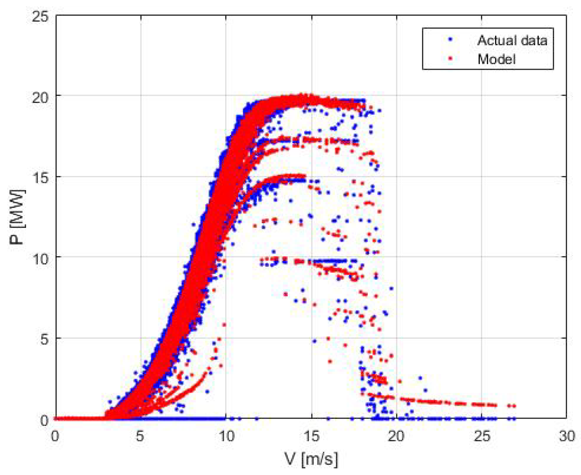
A total of 1440 various neural networks were tested to forecast electricity production from wind power plant FW1. Figure 17 includes the measured and predicted power characteristic depending on wind velocity for which the MAE (3)/MAPE (6) error was the smallest.
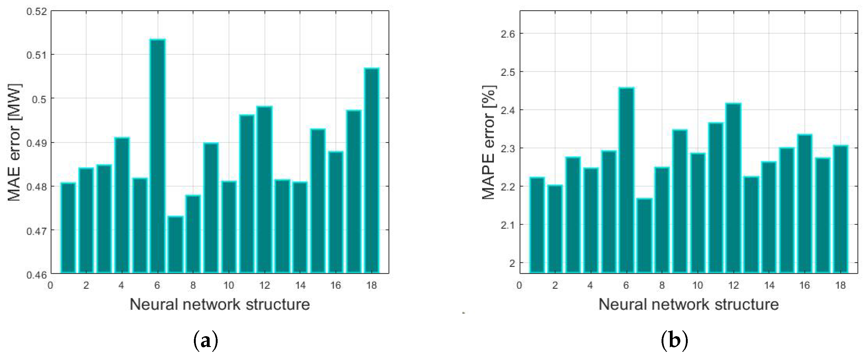
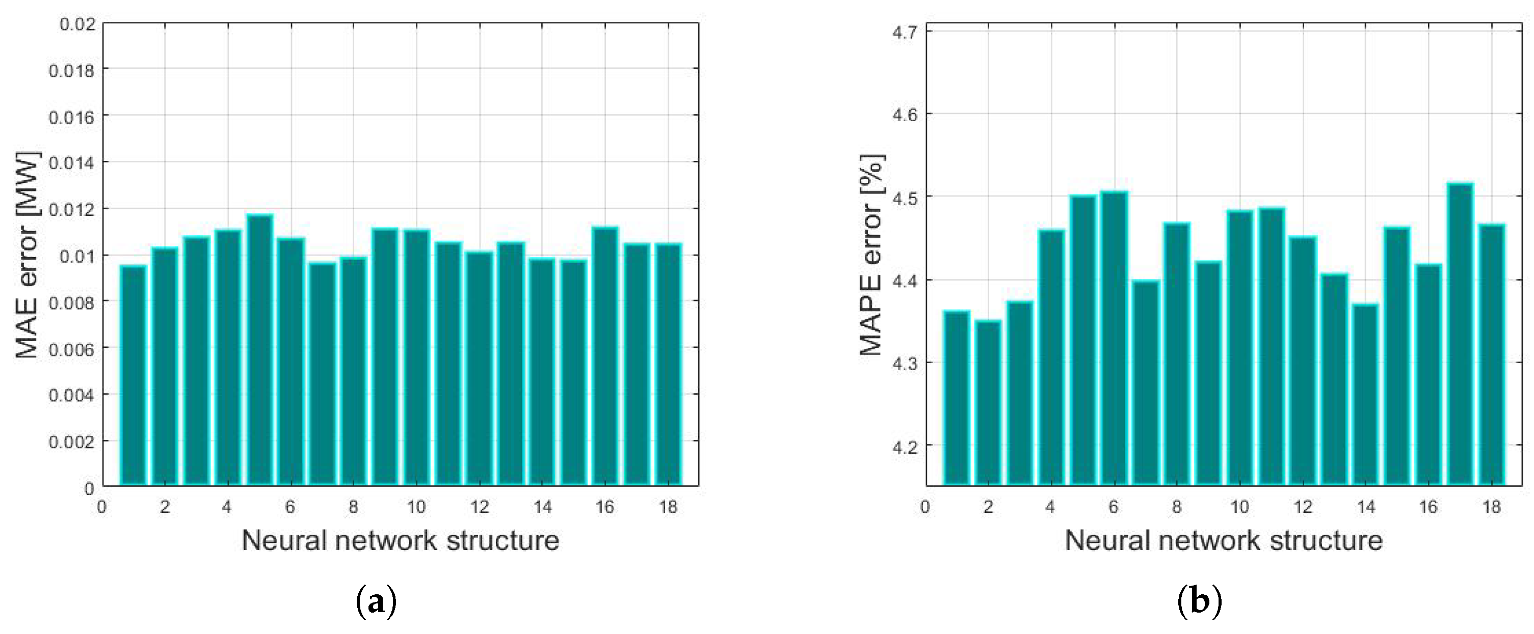
The forecasts were generated for the input data set and network structure in accordance with Table 4 and Table 5 for wind power plant FW1. The comparison of the forecasting accuracy in terms of the mean absolute error (MAE) depending on the neural network structure is shown in Figure 18.
Figure 18a,b show the comparison of the forecasting accuracy in terms of the MAE and MAPE error, depending on the neural network structure.
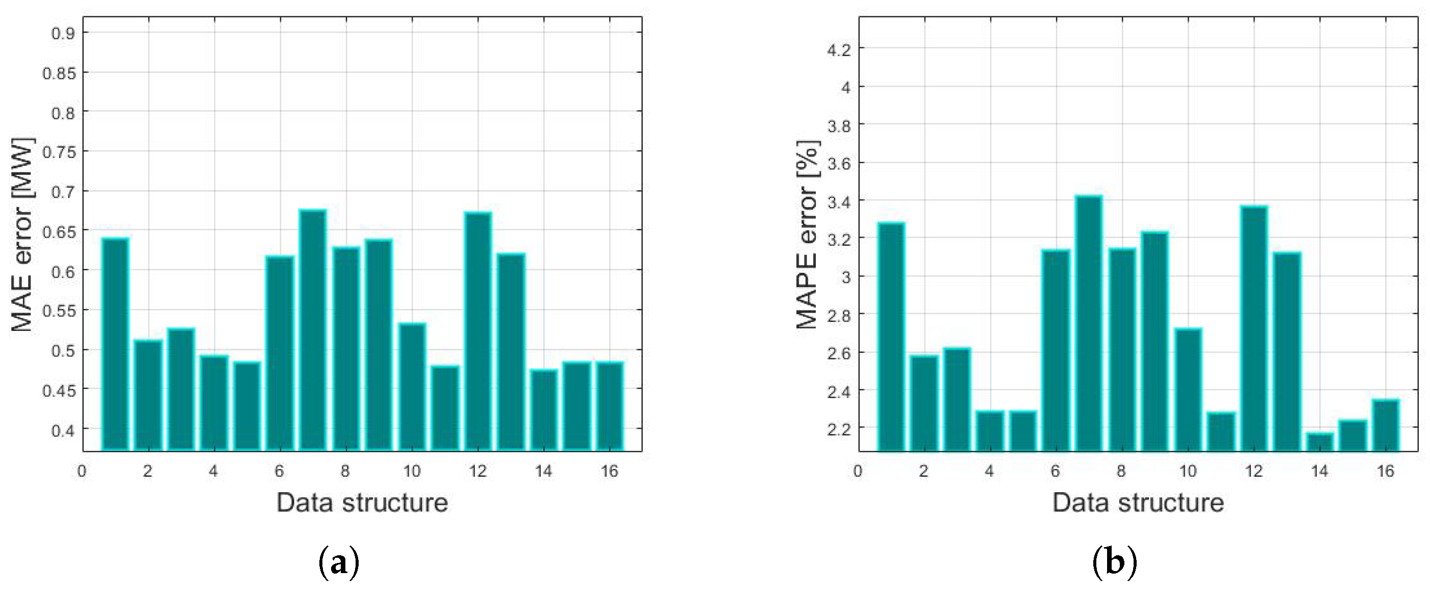
Figure 19a,b show the comparison of the forecasting accuracy in terms of the MAE and MAPE error, depending on the selected data structure.
It follows from Figure 18 and Figure 19 that the forecasts for wind power plant FW1 show the greatest accuracy for data structure No. 14 and network structure No. 7, depending on the selected MAE/MAPE forecast error.

3.1.2. Wind Power Plant FW2

The forecasts were generated for the input data set and network structure in accordance with Table 4 and Table 5. A total of 270 different neural networks were tested for that purpose. The comparison of wind power plant FW2 production forecasts with the as-measured value is shown in Figure 20.
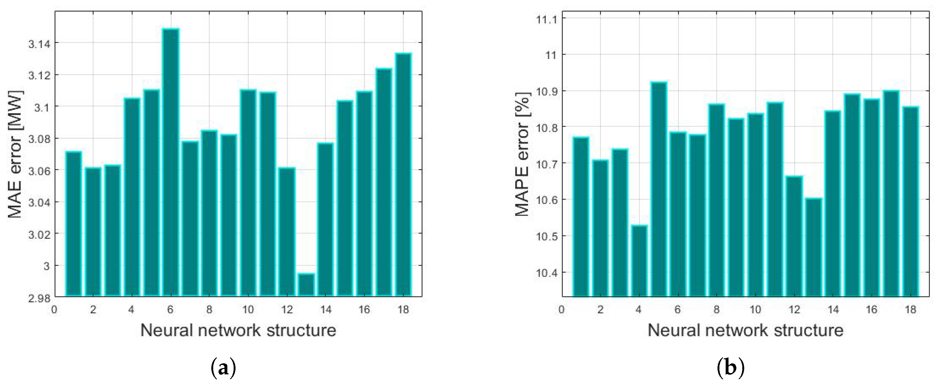
The comparison of the forecasting accuracy in terms of MAE and MAPE depending on the neural network structure is shown in Figure 21.
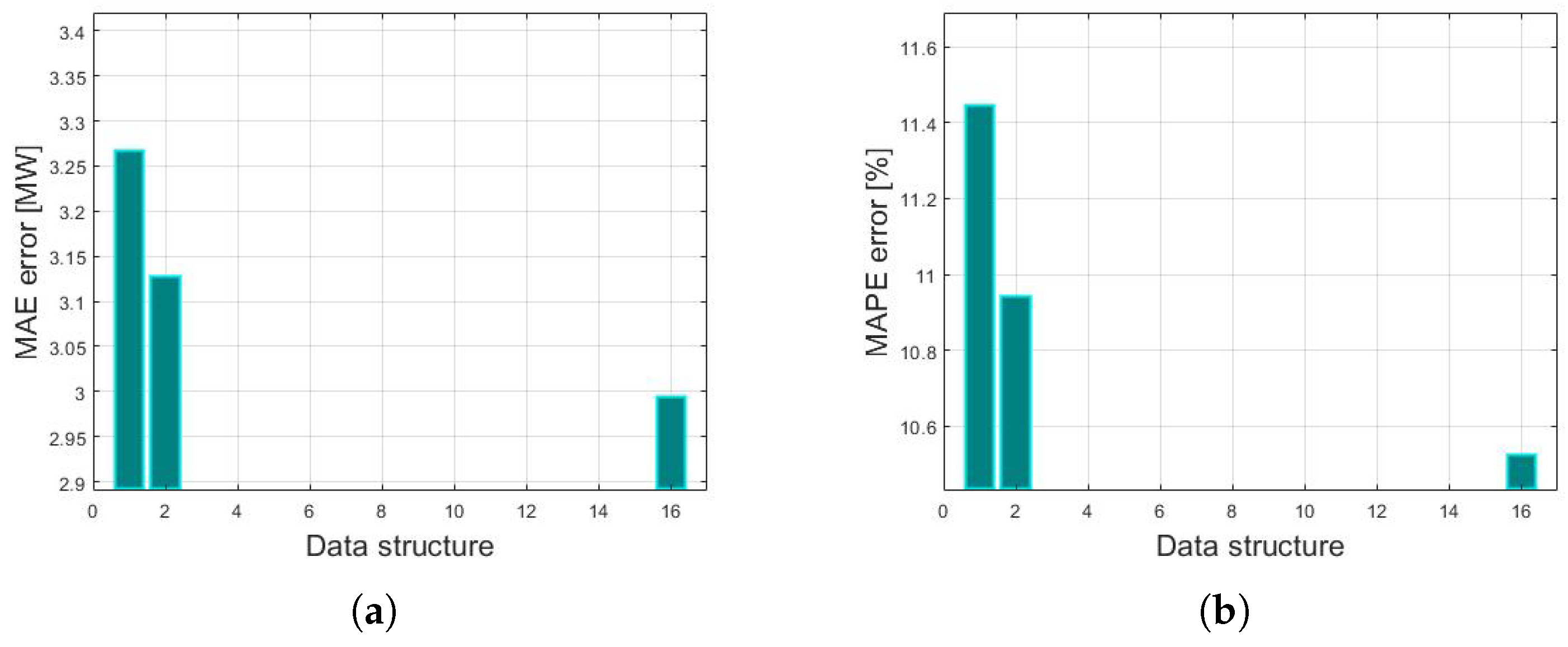
Figure 22a,b show the comparison of the forecasting accuracy in terms of the MAE and MAPE error, depending on the input data structure.
It follows from Figure 21 and Figure 22 that the forecasts for wind power plant FW2 show the greatest accuracy for data structure No. 16 and network structure No. 13/4, depending on the selected MAE/MAPE forecast error.

3.1.3. Wind Power Plant FW3

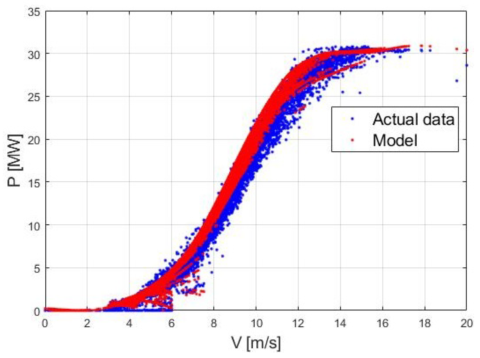
The input data set for wind power plant FW3 includes wind velocity and direction, number of turbines working, and month. The input data set in stock enabled analysis for the data structure is included in Table 5. A total of 450 various neural networks were tested to forecast electricity production from wind power plant FW3. The forecasts were generated for the input data set and network structure in accordance with Table 4 and Table 5 for wind power plant FW3. The summary of forecasts and recorded power–wind velocity relation is shown in Figure 23.
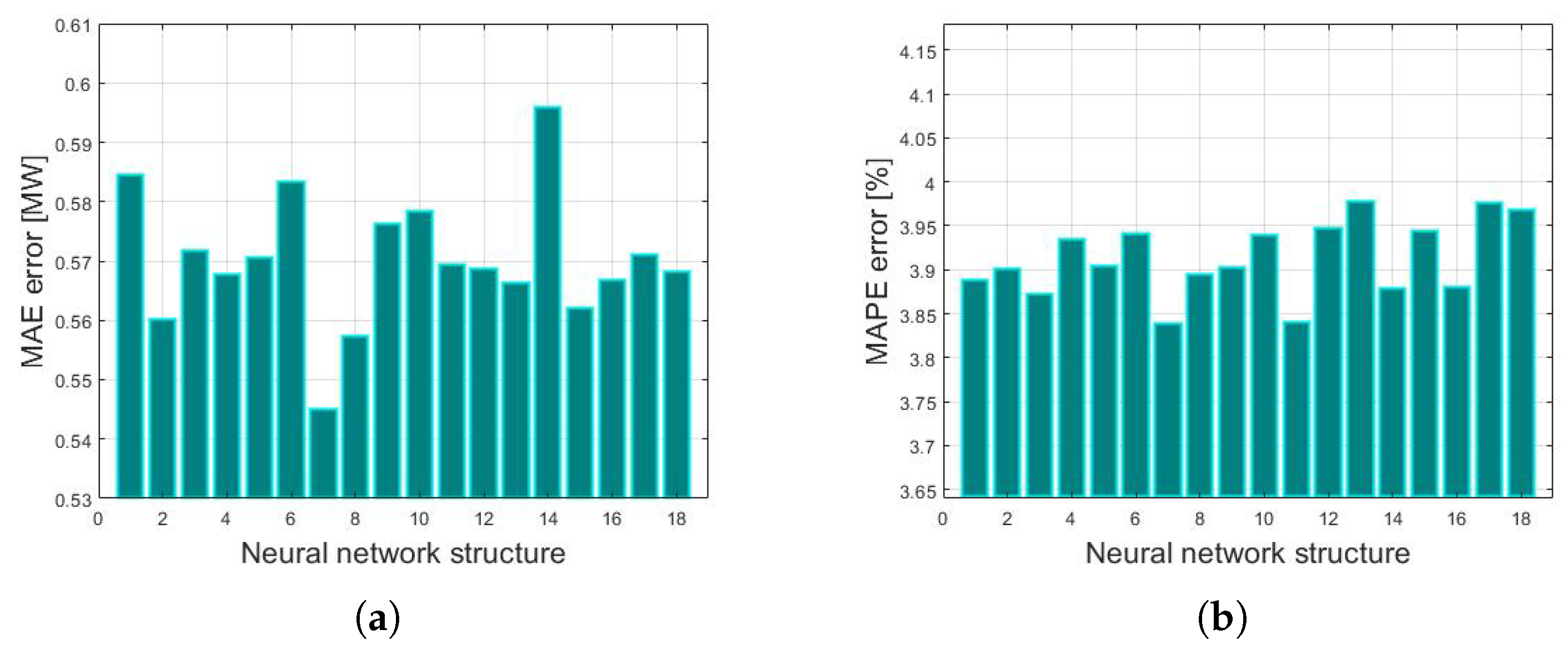
Figure 24 shows the comparison of the forecasting accuracy in terms of MAE and MAPE depending on the tested neural network structure.
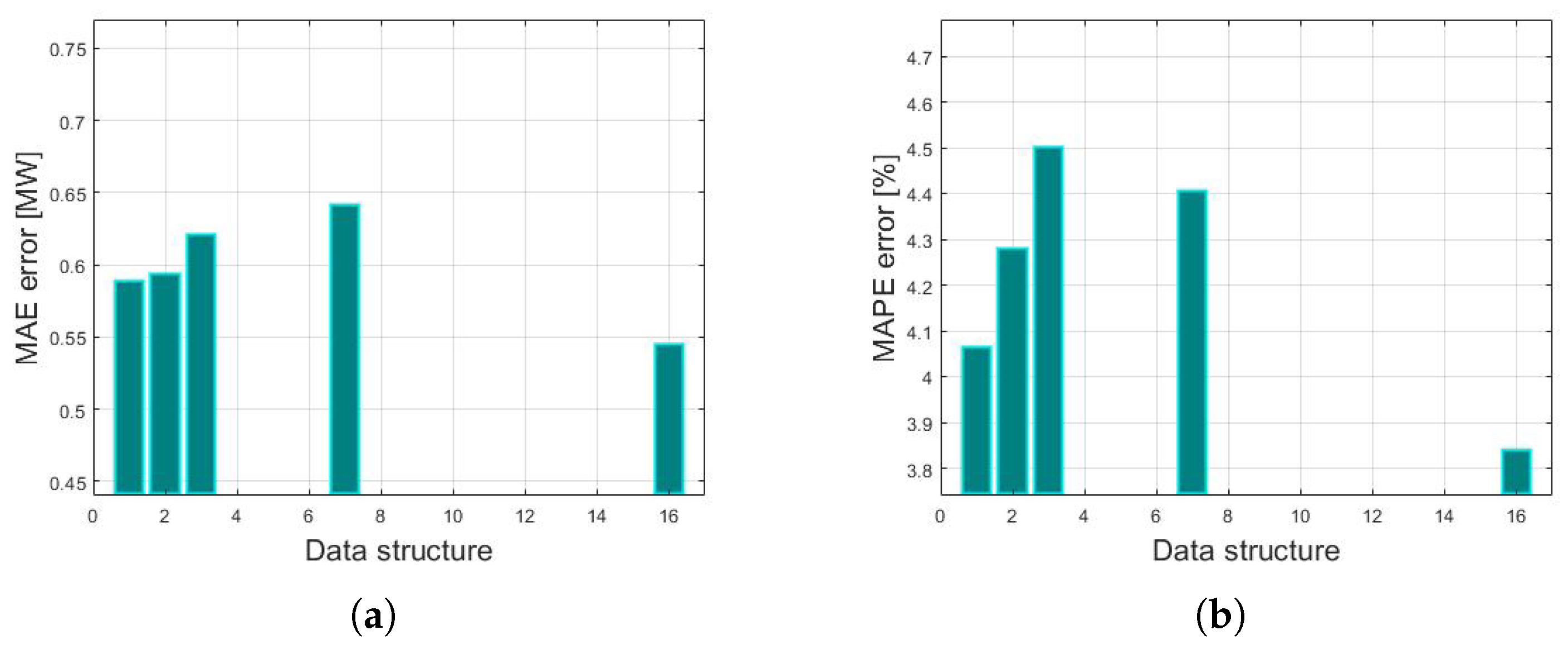
Figure 25a,b show the comparison of the forecasting accuracy in terms of MAE and MAPE depending on the input data structure.
It follows from Figure 24 and Figure 25 that the forecasts for wind power plant FW3 show the greatest accuracy for data structure No. 16 and network structure No. 7, regardless of the selected MAE/MAPE forecast error.

3.1.4. Wind Power Plant FW4

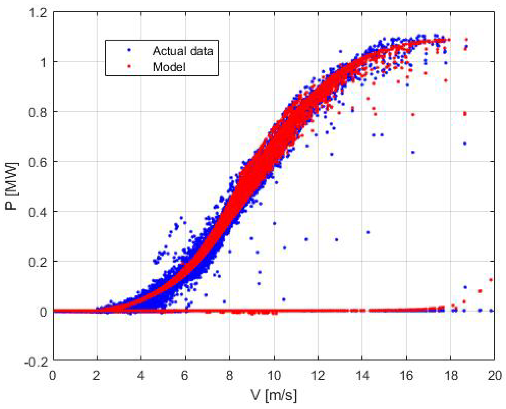
The forecasts were generated for the input data set and network structure in accordance with Table 4 and Table 5 for wind power plant FW4. The input data set for wind power plant FW4 includes wind velocity and direction, number of turbines working, and month. The input data set in stock enabled analysis for the data structure is included in Table 5. A total of 630 various neural networks were tested to forecast electricity production from wind power plant FW4. The comparison with the actual data in Figure 26 shows the accuracy of the proposed model. Figure 27 shows the comparison of the forecasting accuracy in terms of MAE and MAPE depending on the neural network structure tested.
Figure 17, Figure 20, Figure 23, and Figure 26 show a set of points above the power characteristic curve, which may result from the uneven distribution of wind velocity within the power plant, or significant wind velocity variability.
Figure 28a,b show the comparison of the forecasting accuracy in terms of the MAE and MAPE error, depending on the input data structure.
It follows from Figure 27 and Figure 28 that the forecasts for wind power plant FW4 show the greatest accuracy for data structure No. 4 and network structure No. 1 and 2, depending on the selected MAE/MAPE forecast error.
It follows from the analysis that the smallest forecast errors were present for the average-size FW1/FW3 with an output of 20 MW/30 MW, and were below 2.35% (MAPE). Forecast errors for FW4 are greater, but do not exceed 4.4% (MAPE). Increasing the error may result from greater sensitivity of changes in the summary power plant output resulting from variable wind velocity. The effect of averaging out production from the respective turbines is not there as in the case of power plants FW1/FW3, which comprise more than one turbine. If the number of turbines is too big, and input data sets are insufficient, the forecast error increases, as in the case of FW2. The forecast for that object has the largest error in the region of 10.6% (MAPE). In summary, forecast errors for the tested power plants may result from three main factors: the surface area of the power plant, the number of turbines working, and the availability of input data streams for the model.

3.2. Multipoint Adjustment of Wind Power Plant Energy Production Forecast

Data coming from numerical weather forecasts constituting the primary source of information for the RES electricity generation forecast models typically carry errors and inaccuracies resulting from the limited resolution of the forecasting net for weather factors. A method for increasing that accuracy was proposed, so that it comes as close as possible to the actual conditions present in the direct vicinity of the power plant. To that end, NWPs from two different web portals and six points located at a certain distance from the power plant were collected and verified. The proposed multipoint numerical weather forecast adjustment method can increase the wind power plant prediction accuracy.

3.2.1. Multipoint Adjustment of Weather Forecasts

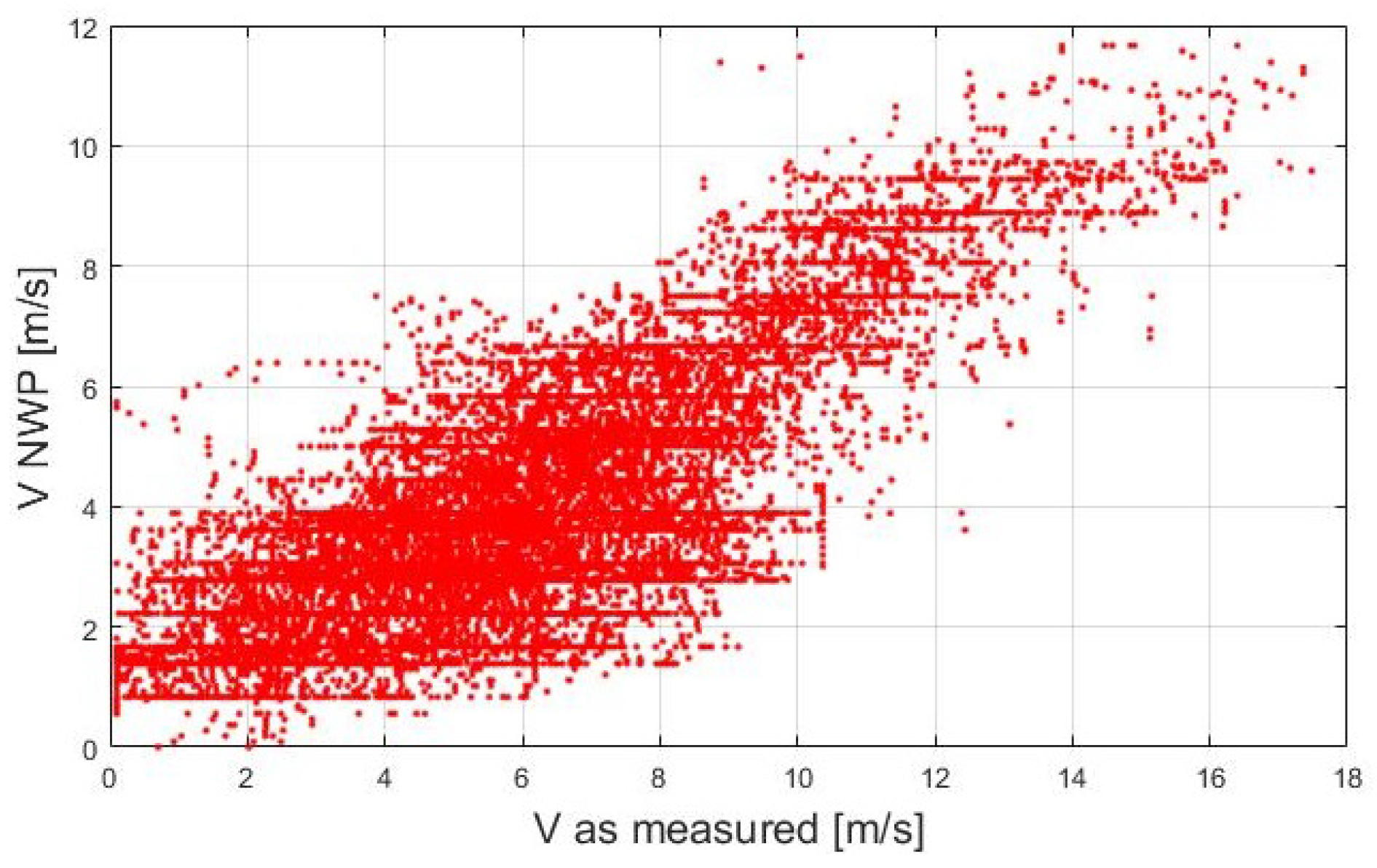
Figure 29 shows the correlation of the wind velocity values as measured and as predicted by NWP for a point located closest to the power plant. It shows significant discrepancies in the wind velocities as predicted and as measured. Non-linear points are distributed over the surface area of the drawing. The greatest discrepancies are for the as-measured wind velocities of 4–10 m/s. In this range, NWPs show the greatest distribution of points on the vertical axis relative to the as-measured values. In this range, the power plant’s power characteristic is strongly non-linear, which is an additional hindrance to prediction, increasing its errors.
To increase the forecast accuracy, the development of a dedicated neural network was proposed, intended to adjust numerical weather forecasts. The neural network is based on data coming from multiple points located in the vicinity of the power plant. In addition, data from two weather portals that make available NWP data, such as wind velocity and direction, ambient temperature and dew point, and pressure and humidity, were used for the forecast. The input data structure was compared independently, with MAE and MAPE prediction error as the criterion.
A total of 1800 neural networks were tested for the FW4 power plant wind direction forecast adjustment. A total of 30 neural network structures were proposed for the forecasting, from two to four layers, and with 5–45 neurons in the layer (Table 6).
Networks containing a greater number of neurons and layers require a specially developed computational unit for the computations. The server was fitted with two four-core 3.00 Ghz chips and 32 GB of operating memory. Despite those parameters, the time to find the network weights matrix was, on many occasions, longer than 1 h.

Selection of the Neural Network Structure

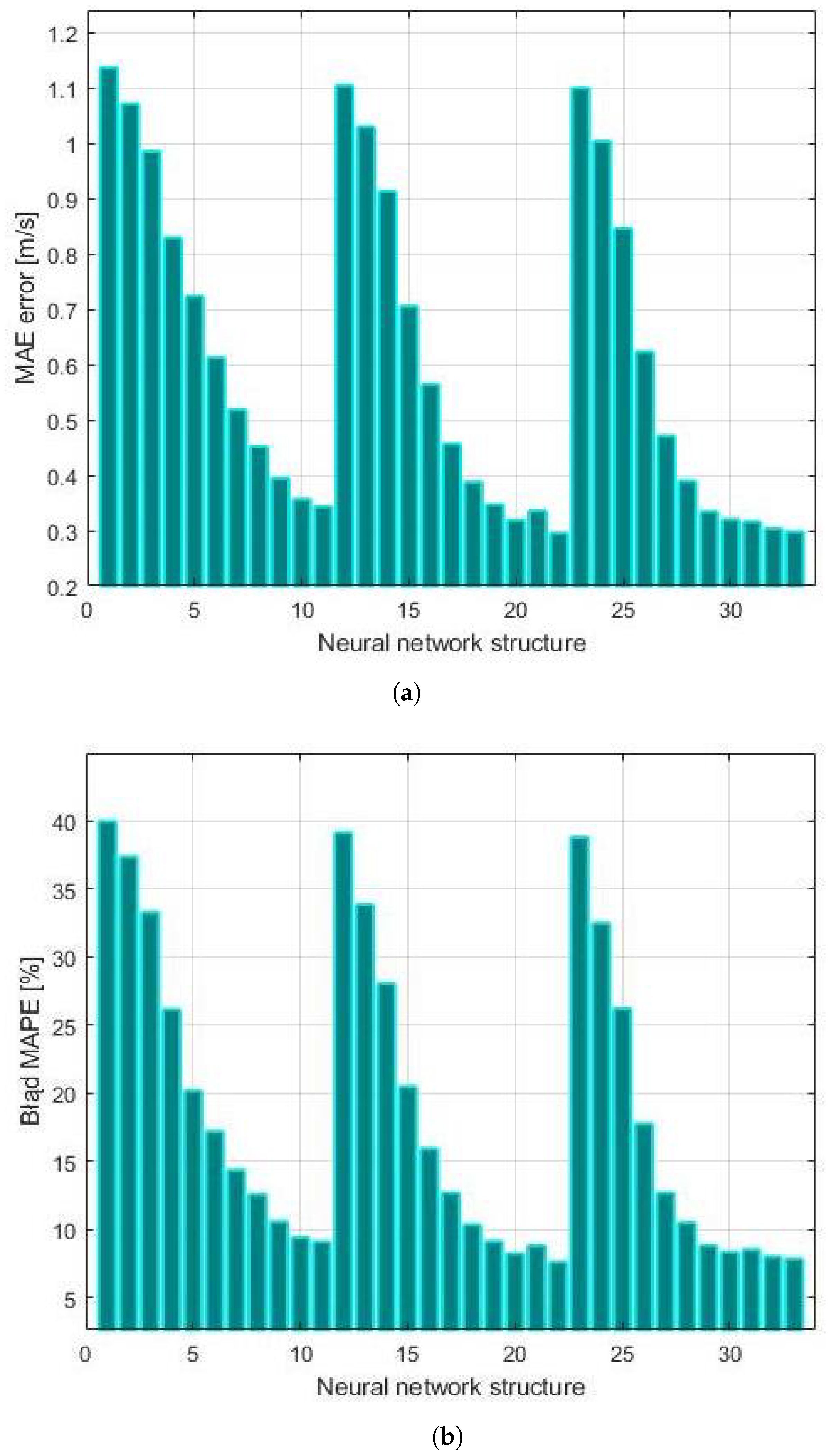
The comparison of the forecasting accuracy (wind velocity and temperature) in terms of MAE and MAPE error depending on the neural network structure is shown in Figure 30a,b, respectively. The figures show the impact of the number of neurons on the forecasting error. The more neurons, the closer the adjusted wind velocity value was to the as-measured value.
A further increase in the number of neurons for structures 19 and 20 did not improve forecasting accuracy. A change in the number of hidden layers involves longer network learning processes, and translates into prediction quality to a limited extent only.
Table 7 shows the numerical summary of the absolute prediction error for wind velocity relative to as-measured values.

Input Data Structure Selection

A total of 12 data structures containing information from six points located in the vicinity of the power plant were proposed for the forecast, coming from two different numerical weather forecast models. In the following data structures from 1 to 6, the input information for the neural network was amplified by the predicted wind velocity for the subsequent forecasting point. Data for structures 1–3 come from one weather portal, and for structures 4–6, from another weather portal (Table 8).
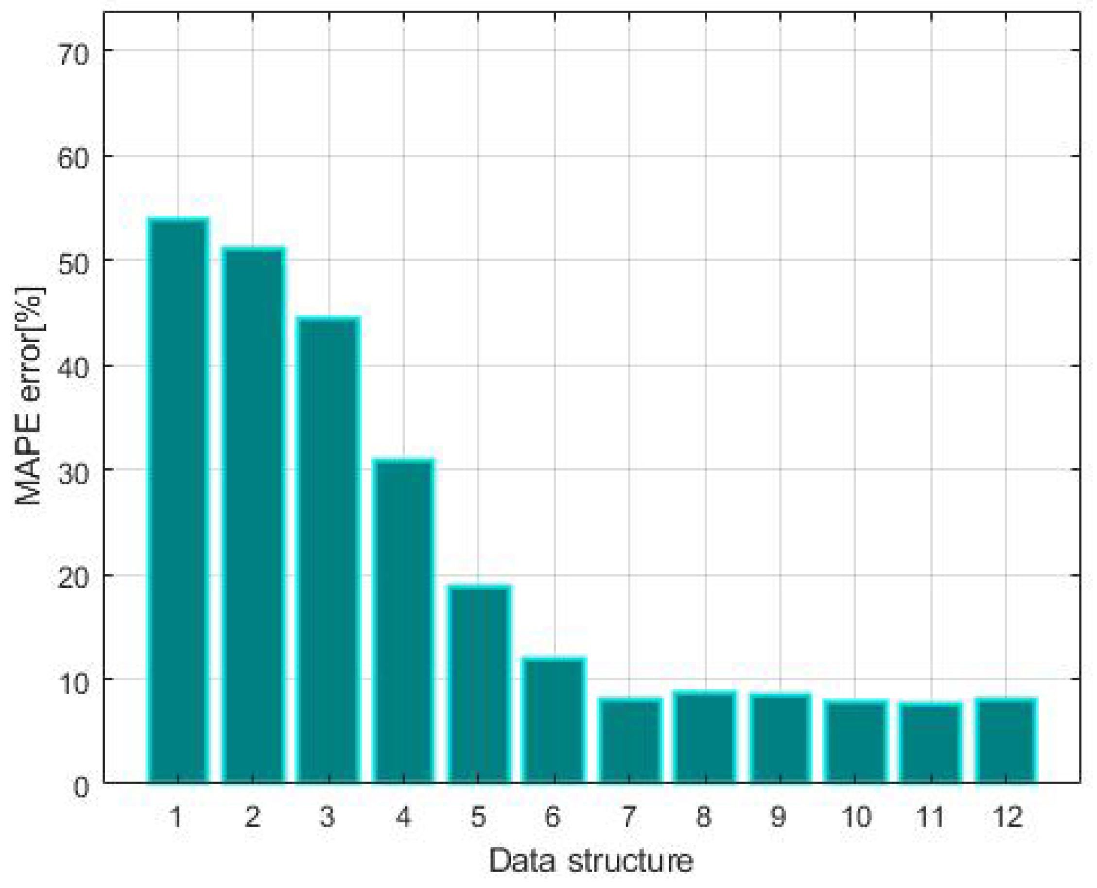
Figure 31 shows the impact of the input data structure change on the quality of the wind velocity adjustment expressed as MAE error. Figure 32 shows the impact of the input data structure change on the quality of the wind velocity adjustment expressed as MAPE error.
It follows from Figure 31 and Figure 32 that adding information from another weather portal (structure 4–6) can reduce the MAE error by more than 60%, and MAPE error by more than 70%. Adding an additional piece of information about the temperature at the respective points can reduce the forecasting error by another 5–8%.
A useful summary is the matrix of the mutual correlations of input data, provided in Table 9. A strong relation between the predicted wind velocities (generated using NWP–V p1–p6) and the as-measured values V p0 can be seen. The correlation of the predicted temperatures T p1–p6 with V p0 is clearly weaker. That confirms a smaller impact of temperatures on the forecasting accuracy is also shown in Figure 31 and Figure 32.

3.2.2. Energy Production Forecasting Using Multipoint Weather Forecast Adjustment

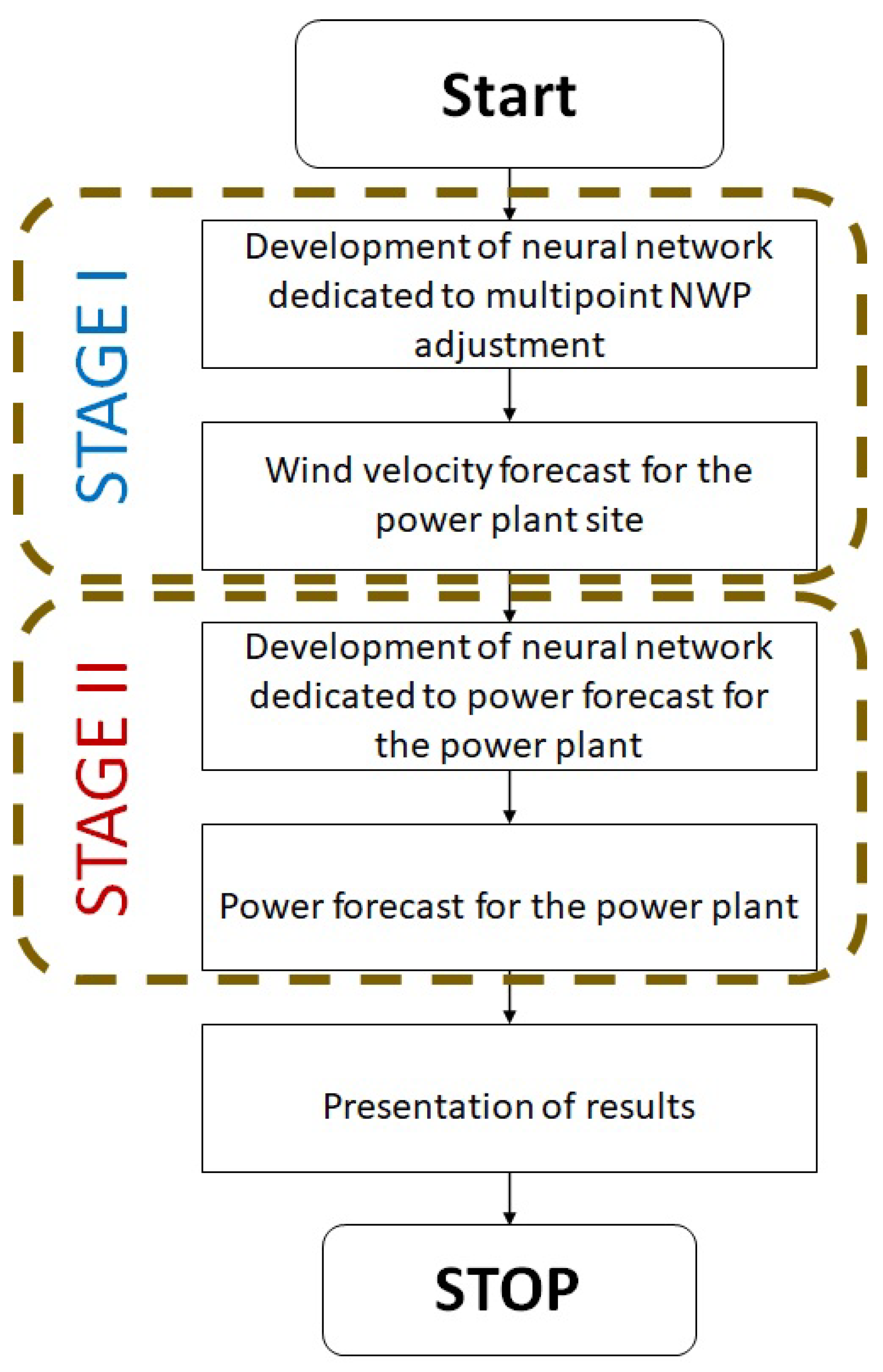
Energy production forecasting using multipoint weather forecast adjustment comprises two steps. The first is the adjustment of the predicted wind velocity values using NWP models. In this step, forecast data are correlated with as-measured values, coming from the weather station installed in the turbine nacelle. The second stage is the power plant output forecasting, described in detail in Section 3.1. The block diagram showing the operating principle of the forecasting system is shown in Figure 33.
On the basis of simulations presented in the section of the paper that covers the selection of the neural network, it can be concluded that the best tool for the pre-processing of data is model No. 19 (3 hidden layers and 45 neurons in the layer) and No. 30 (4 hidden layers and 40 neurons in the layer). A simpler model was chosen as an alternative (three layers with five neurons each), characterized by a greater error, in order to determine the significance of the neural network selection as an impact factor.
For the above models, adjusted wind velocity forecasts for the power plant site were prepared. One-half of the set was used as a learning set to prepare the power forecast model. The proposed neural network comprised three hidden layers, with 15 neurons each. The other half of the prepared data set was used to verify the operation of the models.
Four power forecast models were prepared:
  • Network I—it is a neural network model prepared to verify the operation of the network, using multipoint data adjustment for forecasting. Wind velocity for a point located closest to the power plant was provided as input using NWP.
  • Network II—it is a simple neural network model, comprising three hidden layers, with five neurons in each. Adjusted wind velocity forecasts from six points for the power plant site were provided as the input.
  • Network III—it was selected on the basis of comparisons between the models presented in Figure 30a,b in the section of the paper that covers the selection of the neural network, as a structure showing a small MAE and MAPE error.
  • Network IV—similarly to network III, it was selected as an alternative on the basis of comparisons between the models presented in Figure 30a,b in the section of the paper that covers the selection of the neural network, as a structure showing a small MAE and MAPE error.
Power forecasts were prepared and compared to the as-measured values, and prediction errors for the respective networks (I–IV) are summarized in Table 10.
Figure 34 presents the results of the operation of neural networks I–IV as described above.
Figure 34a shows the relation between the as-measured value and the wind velocity forecast using NWP. The relation is strongly non-linear, which means that a single forecast developed on the basis of the numerical weather forecast may not be sufficient to predict the power plant output. That is confirmed by Figure 34b, presenting the as-measured power characteristic of the power plant, and values predicted by Network I. The forecast results do not overlap with the as-measured values for a significant part of the area. The MAE error for that network is the greatest, at 101.3 [kW], which corresponds to ca. 10% of the wind power plant’s installed capacity. Figure 34c shows the effects of the network’s work when it uses the multipoint weather forecasts on the adjustment of wind velocity forecast at the elevation of the wind turbine nacelle. In this case, similarly to Network I, the correlation between the adjusted wind velocity value and the as-measured values is low. Figure 30a,b show that the number of neurons in the respective layers has a significant impact on the model accuracy. The quality of the adjustment translates directly into the quality of power forecasts developed by the network at the second stage of the system’s operation. The forecast result is slightly better in visual (Figure 34d) and computational (Table 10) terms. The MAE error for that network is 79.9 [kW], which corresponds to ca. 8% of the wind power plant’s installed capacity. Networks III and IV show markedly better forecast results. Even though their structure is different (three and four hidden layers), they allow the generation of forecasts of similar accuracy. A smaller number of layers primarily limits the neural network learning time. In Figure 34e,g, the relation of the adjusted wind velocity and the as-measured value is more linear than for Networks I–II. This confirms that the multipoint adjustment is suitable for the generation of adjusted values, such as wind velocity. Power forecasts (Figure 34f,h) overlap much better with the as-measured power characteristic of the power plant. In comparison to the previous networks, MAE decreased to 34.8/33.4 [kW], which represents around 3% of the power plant’s installed capacity.

4. Discussion

The properties of neural networks used for the forecasting of energy production by their plant enable them to incorporate, in a natural manner, external factors and, where necessary, the related dependencies. In the case of power plants spread over a large area, weather conditions at various points may be different, for example, local overshadowing by clouds, wind deflection caused by terrain shape, etc. It should be remembered that weather forecasts prepared using numerical models are averaged data generated for a given point of the forecasting net. In effect, the information does not include local conditions. Neural network learning using historical data allows the production of a model that takes into account local factors. A summary of the simulation results was prepared on the basis of the analysis, presented in Table 11.
It follows from Table 11 that even though the same set of neural network structures was used and tested each time, the most advantageous configurations of the number of neurons and layers were different. The facilities were selected so that they showed individual properties, such as the installed capacity, the size of the power plant, and its location.
The analysis covered the selection of the input data structure used for the forecast. Furthermore, in this case, different structures could be observed depending on data availability. It could also be observed in the course of the analysis that adding ambient temperature improves forecasting accuracy. In turn, adding pressure as a parameter results in greater noise and the likelihood of erroneous forecasts. Big errors are more frequent.
An important factor that affects forecasting accuracy is the availability of accurate and complete data. Their synchronization over time is also an important factor. The data used in the learning process often come from different measuring devices without a time synchronization system. Artificial neural networks dedicated to energy production forecasting are intended to find a function that approximates the power plant’s power characteristics. It follows from the analysis that the networks allow the approximation of any multi-dimensional, non-linear function. It is both a relatively easy and time-consuming process. The proposed neural networks are able to capture the relations in the power plants.
The result of the work was a forecasting application dedicated to wind farms. More information about the application has been added in the Appendix A.

5. Conclusions

The analysis of the impact of weather factors on the output of the RES power plant allowed us to select the input data set structures and improve forecasting accuracy. The best data structures and networks for various power plants were selected. An individual forecasting model should be built for each power plant. As shown in Figure 18, Figure 21, Figure 24, and Figure 27, larger forecast errors occur for large power plants and those consisting of one turbine. The error increases as the plant/capacity area increases. The largest MAPE error was obtained for a 120 MW wind farm and amounted to less than 11%. On the other hand, for 20 MW/30 MW medium power plants, the MAPE error was below 3%. For a single turbine, a slightly larger MAPE error of less than 5% can be seen compared to medium-sized power plants. Therefore, in the case of larger power plants, in order to increase the accuracy of the model, it may be necessary to divide the power plant into smaller, more homogeneous areas, e.g., in terms of land orography. The method of multipoint weather forecast correction proposed in the article allowed the reduction in NMAPE errors from 10% (network I) to 3.3% (network IV). Similarly, the MAE error decreased almost three times from 101.3 [kW] to 33.4 [kW] (Table 10), which confirms the effectiveness of the method. The limitations of the proposed method include the following:
  • Selection of the appropriate data aggregation period, e.g., 10 min/15 min. The increase in data resolution increases the resolution of forecasts;
  • Guaranteeing a sufficiently large set of training data. It is also necessary to take into account the fact that an excessively large training set may also reduce the quality of the forecast;
  • Preparation of an individual model for each power plant;
  • Division of a large power plant into smaller areas, which will be the subject of further research by the authors;
  • Selection—based on our experience—of an appropriate training and verification data set;
  • Arbitrary selection—in the multipoint method—of NWP forecasting grid points located at a certain distance from the power plant.
The neural network models proposed in the paper enable forecasts that are comparable, and often better than the models developed by other centers, which confirms that they are effective.
Future actions will focus on two aspects that will improve forecasting accuracy:
  • Data pre-processing: proper data preparation impacts both the network learning process itself, and the accuracy of the models. Useful data are collected in different databases, as demonstrated by the analysis described in this paper. It does happen that some data are missing regardless of continuous recording of the power plant’s operating parameters using SCADA systems. It is necessary to find the records and amplify them as necessary. An important aspect is also the filtering of the recorded data coming from the power plant. Preparation of the learning and verification data set is also important;
  • Finding a method to improve the accuracy of NWP forecasts and adapt them to the working characteristics and size of the power plant. Numerical weather forecasts are typically generated with limited resolution of the forecasting net, and for elevations of 10 m over the ground level. Power plants are typically located over large areas. In the case of wind power plants, an additional factor to consider is, for example, the elevation of the hub’s axis and wing length.

Author Contributions

Conceptualization, M.D. and Z.H.; Methodology, M.D. and B.Ś.; Formal analysis, M.D.; Investigation, M.D.; Data curation, B.Ś.; Writing—original draft, M.D.; Writing—review & editing, B.Ś.; Visualization, M.D.; Supervision, Z.H.; Project administration, Z.H.; Funding acquisition, Z.H. All authors have read and agreed to the published version of the manuscript.

Funding

The project is co-financed by the National Center for Research and Development as part of research and development work within the Social and economic development of Poland under conditions of globalizing markets GOSPOSTRATEG/ agreement No. Gospostrateg1/385085/21/NCBR/19.

Data Availability Statement

Not Applicable.

Conflicts of Interest

The authors declare no conflict of interest.

Abbreviations

The following abbreviations are used in this manuscript:
AEAbsolute error
ANNArtificial neural networks
ARIMAAutoregressive integrated moving average
ARMAAutoregressive moving average
BABat algorithm
BSABird swarm algorithm
IGFCMImproved gray wolf optimizer based on fuzzy C-means clusters
LSLeast-squares
LS-SVMLeast-squares support vector machines
LSTMLong short-term memory neural network
MAEMean absolute error
MAPEMean absolute percentage error
MLPMultilayer perceptron
MSEMean squared error
NMAPENormalized mean absolute error
NWPNumerical weather prediction
RESRenewable energy sources
RMSERoot mean squared error
RWRFRadar weather research and forecasting
SCADASupervisory control and data acquisition
SDAEStacked denoising autoencoder
SVMSupport vector machine
SVRSupport vector regression
WDWave division
WPPTWind power prediction tool
WPREWind power ramp event
WRFDDeterministic weather research and forecasting
WUWeather underground
XGBoostExtreme gradient boosting

Appendix A

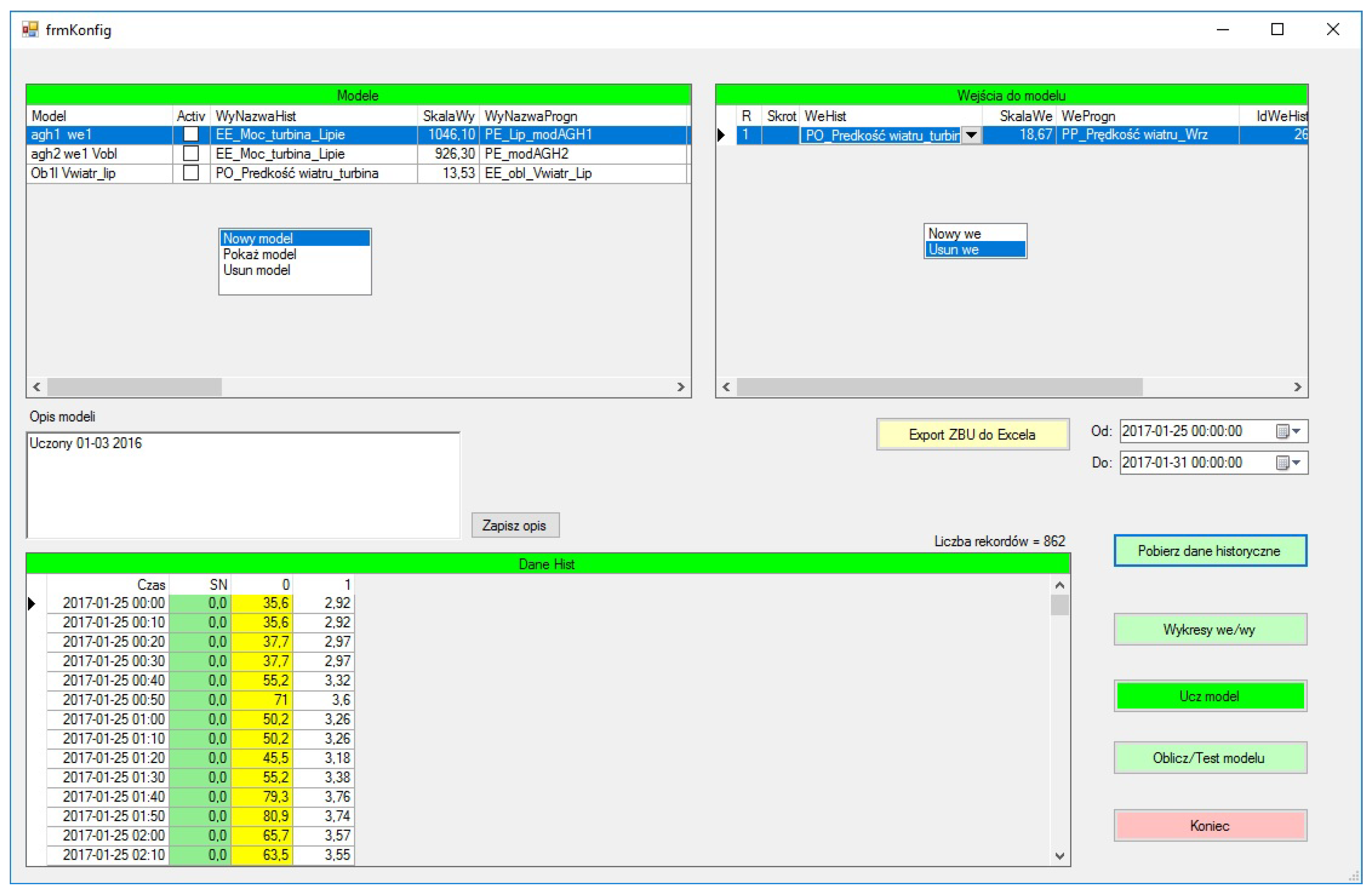
In reliance on their work described here, the authors developed a forecasting application dedicated to energy market companies. The software is dedicated to the forecasting of energy generation in the respective hours for a 24 h horizon on the basis of a defined set of electrical and weather data from the past (for the contemplated renewable source location). Details of the work performed so far are discussed in [53]. Figure A1 shows the main window of the model preparation module.
The tool is used for the forecasting of energy production by wind and solar sources. The system, using artificial intelligence methods, is based on the data collected in an MS SQL database, performing data archiving independently of the SCADA system.
The software is dedicated to the forecasting of energy generation by power plants in the respective hours for a 24 h period on the basis of a defined set of electrical and weather data from the past (for the contemplated renewable source location). The forecasting system using artificial intelligence methods is based on the data collected in an MS SQL database, performing data archiving independently of the SCADA system.
Figure A1. Main window of the model preparation module.
Energies 16 02562 g0a1
The application is intended for the development of power generation forecasts for wind power plants or PV systems. Artificial neural networks are used for forecasting. The learning takes place on the basis of data collected from the local SCADA system and weather data collected from a public-access weather portal. Custom software is prepared for both cases. The input data for the forecasting model is developed on the basis of multiple public-access weather forecasts.

References

  1. IRENA. Renewable Power Generation Costs in 2020; International Renewable Energy Agency: Abu Dhabi, United Arab Emirates, 2021. [Google Scholar]
  2. Enevoldsen, P.; Permien, F.H.; Bakhtaoui, I.; von Krauland, A.K.; Jacobson, M.Z.; Xydis, G.; Sovacool, B.K.; Valentine, S.V.; Luecht, D.; Oxley, G. How much wind power potential does Europe have? Examining European wind power potential with an enhanced socio-technical atlas. Energy Policy 2019, 132, 1092–1100. [Google Scholar] [CrossRef]
  3. Jäger-Waldau, A. PV Status Report 2019; European Commission, JRC Science for Policy Report; Publications Office of the European Union: Luxembourg, 2019. [Google Scholar]
  4. Acaroğlu, H.; García Márquez, F.P. Comprehensive Review on Electricity Market Price and Load Forecasting Based on Wind Energy. Energies 2021, 14, 7473. [Google Scholar] [CrossRef]
  5. Nasir, M.; Jordehi, A.R.; Tostado-Véliz, M.; Tabar, V.S.; Amir Mansouri, S.; Jurado, F. Operation of energy hubs with storage systems, solar, wind and biomass units connected to demand response aggregators. Sustain. Cities Soc. 2022, 83, 103974. [Google Scholar] [CrossRef]
  6. Mansouri, S.A.; Rezaee Jordehi, A.; Marzband, M.; Tostado-Véliz, M.; Jurado, F.; Aguado, J.A. An IoT-enabled hierarchical decentralized framework for multi-energy microgrids market management in the presence of smart prosumers using a deep learning-based forecaster. Appl. Energy 2023, 333, 120560. [Google Scholar] [CrossRef]
  7. Mansouri, S.A.; Nematbakhsh, E.; Jordehi, A.R.; Tostado-Véliz, M.; Jurado, F.; Leonowicz, Z. A Risk-Based Bi-Level Bidding System to Manage Day-Ahead Electricity Market and Scheduling of Interconnected Microgrids in the presence of Smart Homes. In Proceedings of the 2022 IEEE International Conference on Environment and Electrical Engineering and 2022 IEEE Industrial and Commercial Power Systems Europe (EEEIC/I&CPS Europe), Salamanca, Spain, 5–7 September 2022; pp. 1–6. [Google Scholar] [CrossRef]
  8. Ozkan, M.B.; Karagoz, P. A Novel Wind Power Forecast Model: Statistical Hybrid Wind Power Forecast Technique (SHWIP). IEEE Trans. Ind. Inform. 2015, 11, 375–386. [Google Scholar] [CrossRef]
  9. He, M.; Yang, L.; Zhang, J.; Vittal, V. A Spatio-Temporal Analysis Approach for Short-Term Forecast of Wind Farm Generation. IEEE Trans. Power Syst. 2014, 29, 1611–1622. [Google Scholar] [CrossRef]
  10. Pinson, P.; Tastu, J. Discussion of “Prediction Intervals for Short-Term Wind Farm Generation Forecasts” and “Combined Nonparametric Prediction Intervals for Wind Power Generation”. IEEE Trans. Sustain. Energy 2014, 5, 1019–1020. [Google Scholar] [CrossRef] [Green Version]
  11. Xie, L.; Gu, Y.; Zhu, X.; Genton, M.G. Short-Term Spatio-Temporal Wind Power Forecast in Robust Look-ahead Power System Dispatch. IEEE Trans. Smart Grid 2014, 5, 511–520. [Google Scholar] [CrossRef]
  12. Yang, L.; He, M.; Zhang, J.; Vittal, V. Support-Vector–Machine-Enhanced Markov Model for Short-Term Wind Power Forecast. IEEE Trans. Sustain. Energy 2015, 6, 791–799. [Google Scholar] [CrossRef]
  13. Yang, M.; Zhu, S.; Liu, M.; Lee, W.J. One Parametric Approach for Short-Term JPDF Forecast of Wind Generation. IEEE Trans. Ind. Appl. 2014, 50, 2837–2843. [Google Scholar] [CrossRef]
  14. Chen, N.; Qian, Z.; Meng, X.; Nabney, I.T. Short-Term Wind Power Forecasting Using Gaussian Processes. In Proceedings of the Twenty-Third International Joint Conference on Artificial Intelligence (IJCAI’13), Beijing, China, 3–9 August 2013; AAAI Press: Beijing, China, 2013; pp. 2790–2796. [Google Scholar]
  15. Yang, M.; Lin, Y.; Zhu, S.; Han, X.; Wang, H. Multi-dimensional scenario forecast for generation of multiple wind farms. J. Mod. Power Syst. Clean Energy 2015, 3, 361–370. [Google Scholar] [CrossRef] [Green Version]
  16. Mao, Y.; Shaoshuai, W. A review of wind power forecasting prediction. In Proceedings of the International Conference on Probabilistic Methods Applied to Power Systems (PMAPS), Beijing, China, 16–20 October 2016; pp. 1–7. [Google Scholar]
  17. Asmine, M.; Brochu, J.; Fortmann, J.; Gagnon, R.; Kazachkov, Y.; Langlois, C.E.; Larose, C.; Muljadi, E.; MacDowell, J.; Pourbeik, P.; et al. Model Validation for Wind Turbine Generator Models. IEEE Trans. Power Syst. 2011, 26, 1769–1782. [Google Scholar] [CrossRef]
  18. Xu, M.; Gu, T.; Xu, J.; Wang, K.; Li, G.; Guo, F. Electromechanical Modeling of the Direct-Driven Wind Turbine Generator Considering the Stochastic Component of Wind Speed. In Proceedings of the 2nd IEEE Conference on Energy Internet and Energy System Integration (EI2), Beijing, China, 20–22 October 2018; pp. 1–4. [Google Scholar]
  19. Carvalho, L.M.; Teixeira, J.; Matos, M. Modeling Wind Power Uncertainty in the Long-Term Operational Reserve Adequacy Assessment: A Comparative Analysis between the Naive and the ARIMA Forecasting Models. In Proceedings of the International Conference on Probabilistic Methods Applied to Power Systems (PMAPS), Beijing, China, 16–20 October 2016. [Google Scholar]
  20. Jun-fang, L.; Bu-han, Z.; Guang-long, X.; Yan, L.; Cheng-xiong, M. Grey Predictor Models for Wind Speed-Wind Power Prediction. Power Sysem Prot. Control 2010, 38, 152–159. [Google Scholar]
  21. Hua, S.; Wang, S.; Jin, S.; Feng, S.; Wang, B. Wind speed optimisation method of numerical prediction for wind farm based on Kalman filter method. J. Eng. 2017, 2017, 1146–1149. [Google Scholar] [CrossRef]
  22. Gao, S.; He, Y.; Chen, H. Wind speed forecast for wind farms based on ARMA-ARCH model. In Proceedings of the 2009 International Conference on Sustainable Power Generation and Supply, Nanjing, China, 6–7 April 2009. [Google Scholar]
  23. Nair, K.R.; Vanitha, V.; Jisma, M. Forecasting of wind speed using ANN, ARIMA and Hybrid Models. In Proceedings of the International Conference on Intelligent Computing, Instrumentation and Control Technologies (ICICICT), Kannur, India, 6–7 July 2017; pp. 170–175. [Google Scholar]
  24. Tian, S.; Fu, Y.; Ling, P.; Wei, S.; Liu, S.; Li, K. Wind Power Forecasting Based on ARIMA-LGARCH Model. In Proceedings of the 2018 International Conference on Power System Technology (POWERCON), Guangzhou, China, 6–9 November 2018. [Google Scholar]
  25. Bhushan Sahay, K.; Srivastava, S. Short-Term Wind Speed Forecasting of Lelystad Wind Farm by Using ANN Algorithms. In Proceedings of the 2018 International Electrical Engineering Congress (iEECON), Krabi, Thailand, 7–9 March 2018. [Google Scholar]
  26. Khodayar, M.; Wang, J. Spatio-Temporal Graph Deep Neural Network for Short-Term Wind Speed Forecasting. IEEE Trans. Sustain. Energy 2019, 10, 670–681. [Google Scholar] [CrossRef]
  27. Xu, A.; Yang, T.; Ji, J.; Gao, Y.; Gu, C. Application of cluster analysis in short-term wind power forecasting model. J. Eng. 2019, 2019, 5423–5426. [Google Scholar] [CrossRef]
  28. Liu, Y.; Sun, Y.; Infield, D.; Zhao, Y.; Han, S.; Yan, J. A Hybrid Forecasting Method for Wind Power Ramp Based on Orthogonal Test and Support Vector Machine (OT-SVM). IEEE Trans. Sustain. Energy 2017, 8, 451–457. [Google Scholar] [CrossRef] [Green Version]
  29. Xu, A.; Yang, T.; Ji, J.; Gao, Y.; Gu, C. Forecasting Short-Term Wind Speed Based on IEWT-LSSVM Model Optimized by Bird Swarm Algorithm. IEEE Access 2019, 7, 59333–59345. [Google Scholar]
  30. Jafarzadeh Ghoushchi, S.; Manjili, S.; Mardani, A.; Saraji, M.K. An extended new approach for forecasting short-term wind power using modified fuzzy wavelet neural network: A case study in wind power plant. Energy 2021, 223, 120052. [Google Scholar] [CrossRef]
  31. Perveen, G.; Rizwan, M.; Goel, N. Comparison of intelligent modelling techniques for forecasting solar energy and its application in solar PV based energy system. IET Energy Syst. Integr. 2019, 1, 34–51. [Google Scholar] [CrossRef]
  32. Bartman, J. Artificial Neural Networks. Available online: http://www.neurosoft.edu.pl/media/pdf/jbartman/sztuczna_inteligencja/NTI1.pdf (accessed on 27 March 2019). (In Polish).
  33. George Edward Pelham Box. Robustness in the Strategy of Scientific Model Building; Academic Press: Cambridge, MA, USA, 1979; pp. 201–236. [Google Scholar]
  34. Madsen, H.; Nielsen, H.A.; Nielsen, T.S. A tool for predicting the wind power production of off-shore wind plants. In Proceedings of the Copenhagen Offshore Wind Conference & Exhibition, Copenhagen, Denmark, 26–28 October 2005. [Google Scholar]
  35. Osowski, S. Data Mining Methods and Tools; BTC: Legionowo, Poland, 2013. (In Polish) [Google Scholar]
  36. Mondello, M.; Liethen, M.M. Load Validation and Forecasting on Systems with DER. In Proceedings of the 48th CIGRE SESSION, Paris, France, 24 August–3 September 2020. [Google Scholar]
  37. Michi, L.; Carlini, E.; Giannuzzi, G.M.; Ortolano, L.; Martarelli, C. Advance Dispatching and real time electric load forecasting featuring data mining techniques. In Proceedings of the 48th CIGRE SESSION, Paris, France, 24 August–3 September 2020. [Google Scholar]
  38. Meng, X.B.; Gao, X.Z.; Lu, L.; Liu, Y.; Zhang, H. A new bio-inspired optimisation algorithm: Bird swarm algorithm. J. Exp. Theor. Artif. 2015, 28, 673–687. [Google Scholar] [CrossRef]
  39. Abellán-Pérez, J.J.; García-Casado, M.; Rodríguez-Aparicio, A. Evolution and improvements in REE renewable energy forecasting systems. In Proceedings of the 48th CIGRE SESSION, Paris, France, 24 August–3 September 2020. [Google Scholar]
  40. Wu, Y.K.; Huang, C.L.; Wu, S.H.; Hong, J.S.; Chang, H.L. Deterministic and Probabilistic Wind Power Forecasts by Considering Various Atmospheric Models and Feature Engineering Approaches. IEEE Trans. Ind. Appl. 2023, 59, 192–206. [Google Scholar] [CrossRef]
  41. Duan, R.; Peng, X.; Li, C.; Yang, Z.; Jiang, Y.; Li, X.; Liu, S. A Hybrid Three-Staged, Short-Term Wind-Power Prediction Method Based on SDAE-SVR Deep Learning and BA Optimization. IEEE Access 2022, 10, 123595–123604. [Google Scholar] [CrossRef]
  42. Ye, L.; Dai, B.; Pei, M.; Lu, P.; Zhao, J.; Chen, M.; Wang, B. Combined Approach for Short-Term Wind Power Forecasting Based on Wave Division and Seq2Seq Model Using Deep Learning. IEEE Trans. Ind. Appl. 2022, 58, 2586–2596. [Google Scholar] [CrossRef]
  43. Yakoub, G.; Mathew, S.; Leal, J. Intelligent estimation of wind farm performance with direct and indirect ‘point’ forecasting approaches integrating several NWP models. Energy 2023, 263, 125893. [Google Scholar] [CrossRef]
  44. Cui, Y.; Chen, Z.; He, Y.; Xiong, X.; Li, F. An algorithm for forecasting day-ahead wind power via novel long short-term memory and wind power ramp events. Energy 2023, 263, 125888. [Google Scholar] [CrossRef]
  45. Jeonghyeon, K.; Asif, A.; Hyun-Goo, K.; Truong, D.C.; Goon, P.S. Wind power forecasting based on hourly wind speed data in South Korea using machine learning algorithms. J. Mech. Sci. Technol. 2022, 36, 6107–6113. [Google Scholar] [CrossRef]
  46. GmbH, E. ENERCON Wind Energy Converters. 2010. Available online: https://www.enercon.de/en/products/ep-2/e-70/ (accessed on 15 February 2010).
  47. Apata, O.; Oyedokun, D. An overview of control techniques for wind turbine systems. Sci. Afr. 2020, 10, e00566. [Google Scholar] [CrossRef]
  48. Yona, A.; Senjyu, T.; Saber, A.Y.; Funabashi, T.; Sekine, H.; Kim, C.H. Application of Neural Network to One-Day-Ahead 24 h Generating Power Forecasting for Photovoltaic System. In Proceedings of the Intelligent Systems Applications to Power Systems, Kaohsiung, Taiwan, 5–8 November 2007; pp. 1–6. [Google Scholar]
  49. Katsigiannis, Y.; Tsikalakis, A.; Georgilakis, P.; Hatziargyriou, N. Improved Wind Power Forecasting Using a Combined Neuro-Fuzzy and Artificial Neural Network Model; Springer: Berlin/Heidelberg, Germany, 2006; Volume 3955, pp. 105–115. [Google Scholar]
  50. Hertz, J.; Krogh, A.; Palmer, R. Introduction to Neural Computations, 2nd ed.; WNT: Warszawa, Poland, 1993. (In Polish) [Google Scholar]
  51. Tadeusiewicz, R.; Gąciarz, T.; Borowik, B.; Leper, B. Discovering Properties of Neural Networks Using C# Programs; Polska Akademia Umiejętności: Kraków, Poland, 2007. (In Polish) [Google Scholar]
  52. Rymarczyk, R. Neural Network Simulation Decisions; Wydawnictwo Wyższej Szkoły Bankowej: Poznań, Poland, 1997. (In Polish) [Google Scholar]
  53. Hanzelka, Z.; Firlit, A. Power Plants with Renewable Sources—Selected Issues; AGH: Kraków, Poland, 2015. (In Polish) [Google Scholar]
  54. Li, J.; Cheng, J.H.; Shi, J.Y.; Huang, F. Brief Introduction of Back Propagation (BP) Neural Network Algorithm and Its Improvement. Adv. Comput. Sci. Inf. Eng. 2012, 2, 553–558. [Google Scholar]
  55. Rusiecki, A. Neural Network Learning Algorithms Resistant to Errors in Data (Algorytmy Uczenia Sieci Neuronowych Odporne na błęDy w Danych). Ph.D. Thesis, Politechnika Wrocławska, Wrocław, Poland, 2007. [Google Scholar]
  56. Marquardt, D. An algorithm for least squares estimation of non-linear parameters. J. Soc. Ind. Appl. Math. 1963, 11, 431–441. [Google Scholar] [CrossRef]
Figure 1. Balancing of the electric power system or local energy communities.
Energies 16 02562 g001
Figure 2. Location of the analyzed facilities on the map of Poland.
Energies 16 02562 g002
Figure 3. The actual as-measured data (in blue) and theoretical data (in red) of wind turbine E70 power characteristics, wind power plant FW3 [46].
Energies 16 02562 g003
Figure 4. The annual deviation from the average electricity production for the respective turbines E1–E15, wind power plant FW3.
Energies 16 02562 g004
Figure 5. As-measured data (in blue) and approximate minimum/maximum power characteristic envelope (red/yellow), wind power plant FW3.
Energies 16 02562 g005
Figure 6. As-measured data (in blue) and approximate minimum/maximum power characteristic envelope (red/yellow), for selected E1, E2, E5, and E15 turbines of wind power plant FW3. (a) Turbine E1. (b) Turbine E2. (c) Turbine E5. (d) Turbine E15.
Energies 16 02562 g006
Figure 7. The neural network structure for the analysis of the impact of external factors on the wind power plant operation.
Energies 16 02562 g007
Figure 8. Wind power plant FW1: (a) power characteristics for T < 5 C i T > 15 C determined using neural networks, (b) power plant power difference for both cases as percentage of the farm’s rated output.
Energies 16 02562 g008
Figure 9. Wind power plant FW3: (a) power characteristics for T < 5 C i T > 15 C determined using neural networks, (b) power plant power difference for both cases as percentage of the farm’s rated output.
Energies 16 02562 g009
Figure 10. Wind power plant FW4: (a) power characteristics for T < 5 C i T > 15 C determined using neural networks, (b) power plant power difference for both cases as percentage of the farm’s rated output.
Energies 16 02562 g010
Figure 11. Wind power plant FW1: (a) power characteristics for p < 997 hPa and p > 1018 hPa, determined using neural networks, (b) power plant power difference for both cases as percentage of the farm’s rated output.
Energies 16 02562 g011
Figure 12. Wind power plant FW1: (a) FW1 power characteristic for wind directions in ranges of 45 degrees, (b) generated power difference for selected wind directions as percent of the farm’s rated power.
Energies 16 02562 g012
Figure 13. Wind power plant FW3: (a) FW3 power characteristic for wind directions in ranges of 45 degrees, (b) generated power difference for selected wind directions as percent of the farm’s rated power.
Energies 16 02562 g013
Figure 14. Wind power plant FW3 wind rose.
Energies 16 02562 g014
Figure 15. Primary structure of the object model.
Energies 16 02562 g015
Figure 16. Neuron model [53].
Energies 16 02562 g016
Figure 17. Data as measured and forecast of energy production from wind power plant FW1.
Energies 16 02562 g017
Figure 18. Summary of forecast accuracies by the selected neural network structure for wind power plant FW1. (a) MAE. (b) MAPE.
Energies 16 02562 g018
Figure 19. Summary of forecast accuracies by the selected data structure for wind power plant FW1. (a) MAE. (b) MAPE.
Energies 16 02562 g019
Figure 20. Data as measured and forecast of energy production from wind power plant FW2.
Energies 16 02562 g020
Figure 21. Summary of forecast accuracies by the selected neural network structure for wind power plant FW2. (a) MAE. (b) MAPE.
Energies 16 02562 g021
Figure 22. Summary of forecast accuracies by the selected data structure for wind power plant FW2. (a) MAE. (b) MAPE.
Energies 16 02562 g022
Figure 23. Data as measured and forecast of energy production from wind power plant FW3.
Energies 16 02562 g023
Figure 24. Summary of forecast accuracies by the selected neural network structure for wind power plant FW3. (a) MAE. (b) MAPE.
Energies 16 02562 g024
Figure 25. Summary of forecast accuracies by the selected data structure for wind power plant FW3. (a) MAE. (b) MAPE.
Energies 16 02562 g025
Figure 26. Energy production forecast for wind power plant FW4.
Energies 16 02562 g026
Figure 27. Summary of forecast accuracies by the selected neural network structure for wind power plant FW4. (a) MAE. (b) MAPE.
Energies 16 02562 g027
Figure 28. Summary of forecast accuracies by the selected data structure for wind power plant FW4. (a) MAE. (b) MAPE.
Energies 16 02562 g028
Figure 29. Correlation of the wind velocity values as measured and as predicted by NWP for wind power plant FW4.
Energies 16 02562 g029
Figure 30. Comparison of neural network structures for wind power plant FW4. (a) MAE. (b) MAPE.
Energies 16 02562 g030
Figure 31. Comparison of data structures for wind power plant FW4, MAE error.
Energies 16 02562 g031
Figure 32. Comparison of data structures for wind power plant FW4, MAPE error.
Energies 16 02562 g032
Figure 33. Block diagram of the adjustment and power forecast system for the power plant.
Energies 16 02562 g033
Figure 34. Measured and predicted output of the power plant. (a) Correlation characteristics of measured and predicted wind velocity—Network I. (b) Power characteristic of the power plant—Network I. (c) Correlation characteristics of measured and predicted wind velocity—Network II. (d) Power characteristic of the power plant—Network II. (e) Correlation characteristics of measured and predicted wind velocity—Network III. (f) Power characteristic of the power plant—Network III. (g) Correlation characteristics of measured and predicted wind velocity—Network IV. (h) Power characteristic of the power plant—Network IV.
Energies 16 02562 g034aEnergies 16 02562 g034b
Table 1. Pearson correlation coefficient, wind direction/FW3 power.
Wind Direction [ ]Correlation CoefficientSet Size
0–450.046167
45–900.1013,863
90–1350.1013,901
135–1800.0910,297
180–225−0.0316,317
225–270−0.0320,823
270–315−0.1913,018
315–360−0.035475
Table 2. Pearson correlation coefficient, additional factors/power plant output.
Correlation Coefficient
Impact FactorsFW1FW2FW3FW4
Ambient temperature [ C]−0.13- *−0.12−0.15
Atmospheric pressure [hPa]−0.24- *- *- *
Wind direction [ ]0.14- *0.050.05
Number of turbines working0.460.460.620.48
Wind velocity [m/s]0.900.920.890.83
* —the factor was not calculated due to data unavailability.
Table 3. Structures of analyzed neural networks.
Number of Neurons in LayersNumber of
No.InputHiddenOutputHidden Layers
1N *512
27
310
415
520
625
7N *513
87
910
1015
1120
1225
13N *514
147
1510
1615
1720
1825
* —number of input neurons N depending on the number of input data streams.
Table 4. Analyzed input data structures, wind power plant.
Data Structure
12345678910111213141516
Wind velocityxxxxxxxxxxxxxxxx
Wind direction xxx x x xxx
No. of turbines xxxx xx xxx
Temperature xxx x xxxxx
Pressure xx xxxxxxx
Month Number xxxx
Table 5. Analyzed data structure configurations (for the tested facilities).
Power PlantData Structure
12345678910111213141516
FW1xxxxxxxxxxxxxxxx
FW2xx x
FW3xxx x x
FW4xxxx xx xx
Table 6. Neural network structure, multipoint forecast.
Number of Neurons in LayersNumber of Hidden Layers
No.InputHiddenOutput
1N *512
27
310
415
520
625
730
835
940
1045
11N *513
127
1310
1415
1520
1625
1730
1835
1940
2045
21N *514
227
2310
2415
2520
2625
2730
2835
2940
3045
* —number of input neurons N depending on the number of input data streams.
Table 7. Comparison of neural network structures, MAE error [m/s].
Number of LayersNumber of Neurons
571015202530354045
21.141.070.990.830.720.610.520.450.390.36
31.101.030.910.710.560.460.390.350.320.34
41.101.000.850.620.470.390.330.320.320.30
Table 8. Analyzed input data structures, wind power plant FW4.
Data Structure
123456789101112
Wind velocityNWP1 *Point 1x
Point 2xx
Point 3xxx
NWP2 **Point 4xxxx
Point 5xxxxx
Point 6xxxxxx
TemperatureNWP1 *Point 1xxxxxxx
Point 2xxxxxxxx
Point 3xxxxxxxxx
NWP2 **Point 4xxxxxxxxxx
Point 5xxxxxxxxxxx
Point 6xxxxxxxxxxxx
* —numerical weather forecast coming from the model made available by the weather portal WU. ** —numerical weather forecast coming from the model made available by the weather portal Dark Sky.
Table 9. Mutual correlations matrix, input data.
Wind Velocity—VTemperature—T
p0p1p2p3p4p5p6p1p2p3p4p5p6
V p 0 1.00-
V p 1 0.781.00-
V p 2 0.760.991.00-
V p 3 0.780.990.981.00-
V p 4 0.790.960.960.951.00-
V p 5 0.640.800.810.820.811.00-
V p 6 0.680.860.880.840.870.751.00-
T p 1 −0.06−0.02−0.02−0.03−0.05−0.08−0.031.00-
T p 2 −0.06−0.02−0.03−0.04−0.05−0.08−0.031.001.00-
T p 3 −0.06−0.02−0.02−0.03−0.05−0.08−0.031.001.001.00-
T p 4 −0.06−0.04−0.04−0.05−0.06−0.09−0.040.990.990.991.00-
T p 5 −0.07−0.05−0.05−0.07−0.07−0.09−0.050.980.980.980.981.00-
T p 6 −0.06−0.04−0.04−0.05−0.06−0.08−0.040.990.990.980.990.981.00
Table 10. Summary of power forecast error for wind power plant FW4.
ErrorNetwork INetwork IINetwork IIINetwork IV
RMSE [kW]140.4117.769.068.3
MAE [kW]101.379.934.833.4
MAD [kW]101.880.935.834.7
MAPE [%]86.088.335.339.6
NMAPE [%]10.18.03.53.3
Table 11. Structures for the tested facilities.
MAE Error
FW1FW2FW3FW4
Network structure713181
Data structure141614
MAPE Error
FW1FW2FW3FW4
Network structure713182
Data structure141614
Disclaimer/Publisher’s Note: The statements, opinions and data contained in all publications are solely those of the individual author(s) and contributor(s) and not of MDPI and/or the editor(s). MDPI and/or the editor(s) disclaim responsibility for any injury to people or property resulting from any ideas, methods, instructions or products referred to in the content.