Abstract
Computer-vision-based separation methods for coal gangue face challenges due to the harsh environmental conditions in the mines, leading to the reduction of separation accuracy. So, rather than purely depending on the image features to distinguish the coal gangue, it is meaningful to utilize fixed coal characteristics like density. This study achieves the classification of coal and gangue based on their mass, volume, and weight. A dataset of volume, weight and 3_side images is collected. By using 3_side images of coal gangue, the visual perception value of the volume is extracted () to represent the volume of the object. A Support Vector Machine (SVM) classifier receives () and the weight to perform the coal gangue classification. The proposed system eliminates computer vision problems like light intensity, dust, and heterogeneous coal sources. The proposed model was tested with a collected dataset and achieved high recognition accuracy (KNN 100%, Linear SVM 100%, RBF SVM 100%, Gaussian Process 100%, Decision Tree 98%, Random Forest 100%, MLP 100%, AdaBosst 100%, Naive Bayes 98%, and QDA 99%). A cross-validation test has been done to verify the generalization ability. The results also demonstrate high classification accuracy (KNN 96%, Linear SVM 100%, RBF SVM 96%, Gaussian Process 96%, Decision Tree 99%, Random Forest 99%, MLP 100%, AdaBosst 99%, Naive Bayes 99%, and QDA 99%). The results show the high ability of the proposed technique -SVM in coal gangue classification tasks.
Keywords:
coal; coal gangue; SVM; object classification; volume visual perception; separation system 1. Introduction
Coal as a primary fossil energy source is still in high demand globally with around 38.5% of the global power sources and around 90% of China’s fossil energy source [1]. The coal mining process goes through different phases, one of which is to separate coal ore from coal gangue which not only increases production efficiency but also helps with environmental protection [2,3,4]. Therefore, it has been an open research topic since the early beginning of using coal in the industry which attracted researchers’ attention and led to many works and several separation techniques varying from manual to mechanical. Manual separation relies on the expertise of workers in distinguishing coal and gangue based on weight differences and visual appearance, but it faces main restrictions involving workers’ health hazards, low production rate, and high time consumption. Mechanical techniques on the other hand improved the efficiency of the separation process but led to environmental hazards [2,5,6]. Overall, traditional separation techniques share the same bases of identifying physical characteristics to carry out the recognition process in different procedures, such as visual characteristics (color, texture, shape, …) [7,8,9,10,11], structural characteristics (density, thermal, …) [12], and others.
Artificial intelligence provides useful solutions in most industrial fields. In the mining industry, plenty of new intelligent tools proved great benefits of using this technology [13] in coal gangue recognition and separation systems, artificial intelligence adds efficient tools that can merge the abilities of the expert workers (vision sense) using computer vision with mechanical abilities (Robotics) for fast separation resulting in production increment [10,11,14].
The analysis of coal and gangue characteristics throughout the development of separation systems leads to different work implementation directions, some separation systems perform image geometric texture features extraction to classify Coal/Gangue, and the geometric features are usually extracted from ordinary images, either by using image processing techniques [5,15,16,17,18] or by using neural network [7,19,20,21,22,23]. There are several works in this direction and promising results were achieved, M. Li and K. Sun [20], proposed the use of LS-SVM as the base and grayscale with texture as the features, the experiment used (500) images of four kinds of Coal/Gangue from two different mines and achieved around (98.7%, 96.6%, 98.6%, 96.6%) recognition accuracy. Dongyang Dou et al. [24], present a Relief-SVM method to perform the coal gangue classification, 12 color features, and 7 textural features were extracted and the Relief-SVM method was employed to find the optimal features and build the best classifier for coal and gangue recognition. The paper tests the coal gangue under several conditions including dry clean surface, wet clean surface, dry surface covered by slime, and wet surface covered by slime. The mean accuracy ranged from 95.5–97% and 94–98%. Qiang Liu et al. [25], proposed an improved YOLOv4 algorithm to perform coal gangue classification, the results of the experiment came out with an accuracy rate and recall rate around 94% and 96% respectively. Feng Hu et al. [26], present multispectral spectral characteristics combined with 1D-CNN to build the recognition method of coal and gangue, by collecting multispectral information of coal and gangue then with the average value of each wavelength position to obtain the spectral information of the whole band, then using SGD with 1D-CNN to build the model, the results came with 98.75% accuracy. However, there are influential severe factors such as visual appearance similarities of coal and gangue, source heterogeneity, dust, and light intensity [2,27,28,29], which affect the geometric features extraction process making it tricky. Therefore, researchers sought to find immune factors that do not affect by these influential factors such as X-ray imaging and thermal imaging.
Eshaq, R.M.A. et al. [27], studied the use of thermal images in classifying coal and gangue and how immune thermal images are against influential factors, image processing was applied for feature extraction with an SVM classifier giving a good classification result with 97.83% accuracy. M S Alfarzaeai et al. [2], also addressed the use of thermal images with convolutional neural network to perform coal gangue recognition, the results showed that using thermal images lead to immunity against coal gangue classification issues such as visual appearance similarities, dust, light intensity, and source heterogeneity, results came out with 97.75% accuracy. Feng Hu, and Kai Bian [30], developed a model using CNN with thermal images for coal gangue separation reaching 100% classification accuracy with 192 training samples and 48 testing samples of similar size and shape. Bohui Xu et al. [31], addressed the thermal behavior of two mineral-type coal gangues under different temperature conditions, and investigated by heating treatment of kaolinite-type coal gangue and illite-type coal gangue based on thermal analysis, X-ray diffraction (XRD), infrared spectroscopy (IR), and scanning electron microscopy (SEM). The experimental results showed good potential benefits of using thermal radiation for coal gangue separation purposes.
Using thermal images is subject to the surrounding environment’s temperature and needs a heating process to neutralize it, making thermal imagining solutions suitable in some parts of the industry such as power stations and big steel factories [2,27]. One factor that is immune to external influences and gives an excellent result at the same time is density. Substance density is the critical factor that distinguishes every substance from others. Coal and gangue, as different substances, certainly have different densities which is an excellent factor to distinguish between them [32,33]. Different approaches were approached to predict the density of samples, such as using X-ray imaging to visualize the density of the samples. Yi Ding Zhao, Xiaoming He [34], addressed the use of X-ray with the acquisition of ray signal and image processing analysis, the method was able to recognize coal from gangue with high accuracy; however, these techniques need a huge power supply and should be contained in special containers to prevent the bad influence of X-ray on the worker’s health [35]. X-rays however, come with some limitations regarding pseudo medium coal with light reflection which is falsely classified as gangue leading to waste of raw coal, Lei He et al. [36] addressed this problem and proposed a dual-view visible light image recognition method that traces the pseudo medium waste coal and identifies it with accuracy reached 95%.
Other approaches use computer vision with laser techniques to perform volume prediction and consequently calculate the density based on volume weight relationship [18,32,33]. However, the laser scanning speed is slow and difficult to utilize in the production line, therefore once again computer vision techniques and neural networks provide solutions for volume prediction. Previous works applied computer vision and neural networks to measure the volume of food or agricultural products such as fruit [37], apple [38], egg [39,40,41,42], beans [43], tomato [44], abalone [45], and ham [46,47]. Reviewing these works shows that they are not suitable for coal gangue situations, as these works depend on the regular geometric shape in calculating the volume, unlike the shape of coal ore; therefore, it was important to look for new technologies that serve the purpose of calculating the density of irregular shape objects. Chen Zhang et al. [32] presented a method to separate coal from gangue based on the density after measuring the volume and the weight using a device that uses a laser with CCD camera during the movement of the samples in the production line using Laser triangulation equations. The experiment has shown that this method is suitable for the recognition of coal and gangue with a size bigger than 10 cm, with a separation accuracy of up to 60%. W.Wang and C.Zhang [33] present a new method to separate gangue from coal based on density calculated from volume using three-dimensional (3D) laser scanning technology based on the laser triangulation method and weight using WOM technology. Xiaojie Sun et al. [48] present a side height calibrated shape from a shading algorithm for volume prediction; they work with samples with sizes of 50 mm to 300 mm, and the proposed algorithm focused on the volume prediction but was not tested with coal gangue separation, there are no results to show the accuracy of the proposed algorithm.
Based on the foregoing, this paper presents a method for coal gangue classification using computer vision algorithms with an SVM classifier. The contribution of this paper focuses on giving the machine the ability to use visual sensors to estimate the ore volume and apply it with weight to classify coal and gangue, the proposed method is robust against the aforementioned influential factors by estimating sample volume perception using three images taken with respect to three different positions. The proposed method takes into consideration the relation between object visual perception in the images and the object’s real volume value in the classification based on volume weight relationship. Weight On Motion (WOM) [33], is used to measure the coal gangue weight, then with the extracted volume perception value(), the SVM classifier performs the classification task which will be called ExM-SVM model.
The development in this work goes in the following steps:
- Collecting the dataset of coal gangue samples by measuring the real volume values using the water displacement method in the lab, and weight values with an electronic scale.
- Comparing several classifiers with the real values dataset to view the classification accuracy which will be the test reference for the efficiency of the predicted values.
- Building 3_Side images dataset of the coal gangue samples to extract the volume perception feature () as a replacement of the real volume values.
- Developing the feature extraction functions that will provide ExM-SVM with predicted values to do classification, and test it with the cross-validation dataset.
- Testing the () values dataset in two testing steps (full dataset testing, and cross-validation dataset testing) and observing the accuracy of coal gangue classification using the same classifier’s test that was used with the real volume values.
- Comparing the proposed work with related works and driving out the conclusion.
2. Materials and Methods
Density of an object is defined as the mass of the object divided by its volume, it is a measurement of the substantial amount that an object contains per unit volume through the Equation (1) [33], where P represents the density of the substance.
Density is beneficial for recognizing different materials, the coal gangue density is between 1.7–1.9 g/cm, whereas the main component of coal is an organic matter and the density of concentrate coal is 1.3–1.5 g/cm [33]. Density can be driven out by volume and weight. As the Weight On Motion (WOM) technology provides accurate weight [32,33]; Therefore, only volume needs to be predicted. Although it is difficult to obtain accurate volume measurements because of the irregularity of coal and gangue shapes; However, it’s not necessary to get accurate values of mass and volume as long as density measurement results’ error holds in a certain range that can still achieve separation between them. Although the predicted volume could suffer from prediction errors, it can reflect the difference in real density between coal and gangue. The efficiency of this principle appears in mines where experts manually separate coal from gangue, when it’s difficult to identify an ore type just by looking, the expert worker holds the ore in hand to tell whether it’s coal or gangue. the expert’s accumulated experience helps him to connect the estimated volume and weight of the ore.
Therefore, to simulate this ability in machines, two major sensors are essential, volume measurement, and weighing sensors. There are many studies and applied products that use mechanical weighing such as quantitative weighing systems applied to tobacco production lines and dynamic weighing technology of vehicles, therefore weighing won’t be an issue in coal mining production lines. The volume prediction technique in this paper is driven by the concept of volume visual perception, and the recognition system consists of two steps, first volume visual perception is represented by an existing value ExM, then classification based on the sample weight and ExM value using the suitable classifier. The first part of the system was done by estimating the volume perception in the 3 Side images of the sample and extracting a feature that describes it using image processing functions, the second part which is classification was done using the SVM model. The recognition system uses three cameras to take 3_Side Images of samples through the production line and uses weight on motion (WOM) [33] technology to measure the weight during sample movement on transmission lines, Figure 1 shows the scenario of the separation system working mechanism.
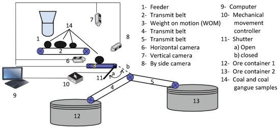
Figure 1.
Separation System parts and separation scenario.
2.1. Dataset Collecting
The dataset was built using 40 samples of coal and gangue (20 coal, 20 gangue), Coal/Gangue samples were collected from Bituminous coal, produced in Shanxi Province west China, and the experiments were conducted at CUMT labs. The real volume of the samples is measured using the water displacement technique by submerging them inside a measured container to measure water volume, then samples volume was determined using the Equation (2):
where is the sample’s real volume, is the water volume with the sample inside it, and is the water volume before submerging the sample inside it. Table 1 shows the real volume measurement of the 40 samples alongside with weight measurement of every sample which was measured using an electronic weight scale. In order to perform volume prediction, 3 Images of samples were captured in different positions (Top, Side, and front) to connect the volume value with the visual perception in the images this dataset called 3_Side images, leading to an increase in the dataset into 810 3_Side Images (451 coal, 358 gangue) in a total of 2430 images, Figure 2 shows the Image acquisition stand. Some samples had fewer 3_Side Images than others because of the irregular shape which had them unable to stand firmly on the capturing flat board such as sample C2 (9 of 3_Side Images) as described in Table 1.

Table 1.
Volume in cm and Weight in g real measurements for coal and gangue using physical methods with 3_side images.
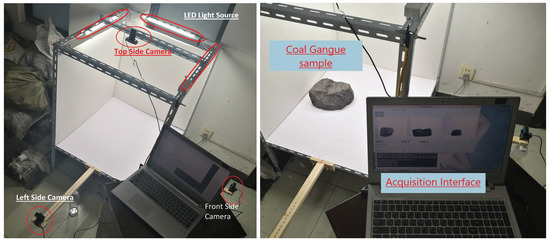
Figure 2.
Capturing Stand Prototype with three USB cameras positions in three sides Top_Side, Front_Side and Left_Side, coal gangue sample, and the Acquisition Interface.
The use of three images to estimate a good perception of the object volume came from the fact that irregular shapes can hide gaps in the shape that reduce the volume, in Figure 3, the Left Side position of the sample has a hidden cavity that is not noticed with the other two images, so the third image comes to show this hidden side of the sample and helps to evaluate the volume perception more accurately.
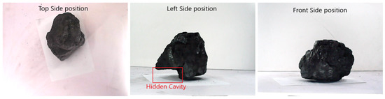
Figure 3.
Samples 3_Side images showing the cavity problem.
2.2. Classifier Selection
For classification tasks, there are several classifiers that vary in the classification methods such as support vector machine which proved solid abilities with small and medium datasets, here in the experiment classification model (ExM-SVM) is used to classify coal and gangue based on the measured weight and volume. For the purpose of finding the suitable classifier, several classifiers were tested (“Nearest Neighbors”, “Linear SVM”, “RBF SVM”, “Gaussian Process”, “Decision Tree”, “Random Forest”, “Neural Net”, “AdaBoost”, “Naive Bayes”, and “QDA”) from the scikit-learn 1.1.3 documentation [49], Table 2 shows the classifiers configuration based on the sklearn details, they have been tested with the collected real measurements of the 40 coal gangue samples volume and the weight to compare the efficiency of the classifiers based on the accuracy and consumed runtime [50], the dataset divided into training group with 70% and testing group with 30%.
Table 2.
Sklearn classifiers configuration details.
Figure 4 shows the results of the different classifier’s Decision Boundaries Display with the Accuracy and Time of training and testing the classifiers, it’s clear that linear_SVM, RBF_SVM, and Gaussian Process achieved 100% of classification accuracy with acceptable classification time, while the rest of the classifiers vary in the classification accuracy and timing. The classifiers show excellent classification results with the real measurements as a result of the linear nature of the data and the clear separatable hyperplane, although, these results lead us into using SVM classifiers, determining the suitable classifier will be based on the results using the extracted features from the 3_side images later, during the two phases of training with the whole dataset and with the cross-validation test.
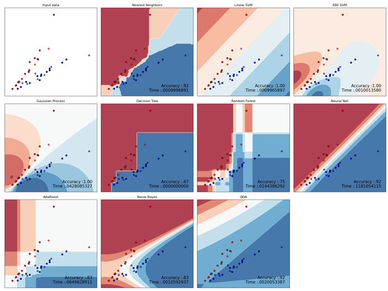
Figure 4.
Real Data of volume and weight values visualization of the two classes (Coal in blue and gangue in Red), trained and tested with “Nearest Neighbors”, “Linear SVM”, “RBF SVM", “Gaussian Process”, “Decision Tree”, “Random Forest”, “Neural Net”, “AdaBoost”, “Naive Bayes”, and “QDA” with the decision boundaries display, classification accuracy in a scale of (0–1) and time in seconds.
2.3. Volume Visual Perception (ExM)
Volume can be described as the amount of space occupied by the object in the image. Despite this, the image shooting angle cannot describe the volume with three dimension occupation as described in Figure 3 due to the hidden cavity problem which hides portions of space that are considered occupied while it is not. So in this study, three different images are used to describe the object volume by calculating the size of the object in every image with the mean of pixels number that the object occupies in the images. 3_side images pass through an image processing function that calculates the existence of the sample in the image , which will be used as a reflection of the volume in the classification step with the classifiers instead of the volume real values. To generate the value out of the images which are input as RGB images first it has been converted from RGB image into grayscale using the Equation (3):
The main principle in this work is object detection and background removal to isolate the object’s presence. This presence is then calculated by counting the pixels, and the obtained value replaces the real volume value in the separation model. Object detection and background removal here is done by detecting object edge lines using Canny Edge detector [51], the result is the image with only the edges of the object with some small objects which could occur during the edge detection process, the fill object function from scikit-image applied to fill the gaps, this gives us an image with two values, either zero for background or ones for the filled objects [52], late the small unwanted objects are detected by specific threshold size equal to 50 pixels, so under this threshold size objects will be removed, Figure 5 shows the steps of background removing for one 3_side image sample, as it mentioned the final output image is an array of ones and zeros values which help the work of estimating the volume perception by counting the ones in the array Equation (4).
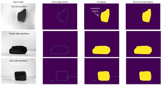
Figure 5.
Image background removing steps: input images (3-side images), Edge detection, gap filling, and unwanted objects removal.
Since the generated images are zero-one images this will reduce the calculation time by only counting the nonzero values in the image. The images are ready for calculating the () value of every image which will be the feature that replaced the volume values in the classification step, () value represents the volume perception in the images by calculating the nonzero pixels of the output image from the last step for the three images and producing the mean of the nonzero pixels of the three images compared to the total number of the pixels in the three images, Equations (4) and (5) explain the calculations of the ().
where represents the object occupation percentage compared to the total image size represented by (width, height), the pixel nonzero value, and is the index of the pixel in the image. later the mean value of the three images Top_side , Left_side , and Front_Side :
by now the volume perception in the three images is represented with () value, later to reduce the difference in the correlation between the extracted value and the sample weight value, the () value is multiplied by 100, this procedure increased the efficiency of the () value. Table 3 shows some of the () extracted values alongside the real volume(R_V) and weight(R_W) values.
Table 3.
Sample of the () values with respect to the real values.
2.4. Evaluation Metrics
The classifiers are evaluated using a classification report from sklearn-metrics library [49], where the report presents a set of calculations that show the accuracy of the classification, and the effectiveness of the classifier, Precision, recall, F1-score, accuracy, macro average, and weighted average are factors to measure the classifier performance, the cases that any class prediction can come with are either True Positive where the predicted class 1 and actual class is 1, True Negative where the predicted class is 1 but actual class is 0, False Positive where the predicted class is 0 where the actual class is 1, and Flase negative where the predicted class is 0 and the actual class is 0. The support value is the sample size of each class in the training dataset. In binary classifications such as coal and gangue, the accuracy is used to measure how well the classification test correctly predicts the classes among the total predictions so it is defined as the ratio between the number of correct predictions and the total number of predictions, Equation (6):
While accuracy measures the true predictions in total, precision, and recall are used to evaluate the class’s predictions, and precision measures the ratio of the true predictions of positive class to the total predictions in positive class which is and the prediction of each class is individually by measuring the ratio of the true positive predictions to the class support number which is the and the , Equation (7):
In the other hand, Recall measures the ratio of the True predictions of the positive class to the actual positive class which could be and , Equation (8):
F1-score is used to measure the harmonic mean of the precision and recall values and is driven by the Equation (9)
The macro average is the arithmetic average of classes evaluation method precision, recall, and F1-score, so in binary classification, F1-score has (F1_0 and F1_1) then the macro average of F1-score driven with Equation (10):
The weighted avg is the arithmetic average of the classes evaluation method with respect to the weight of each class support (WS), let’s take the F1-score weight average for example, first, calculate the WS of each class and then calculate the mean of the classes F1-scores multiplied by there WS, Equation (11):
3. ExM-SVM Model Training and Testing
After collecting and preparing the dataset of the 3_side images and driving out the () value, it is time to test the efficiency of the extracted value as a replacement of the real volume value in the classification task by conducting the previous classifier test but with the () value rather than the volume, and compare the results of the different classifiers classification accuracy alongside the time of the classifier training and testing.
3.1. Experiment Platform
The experiment was done with a hardware platform that comes with CPU A10 PRO-7800B R7, 12 Compute Cores 4C + 8G 3.50 GHz with 4.00 GB installed memory (RAM) and graphic card NVIDIA Quadro K2000 with 2 GB memory data rate (Total available graphics memory 4060 MB, Dedicated video memory 2048 MB GDDR5, Shared system memory 2012 MB), Windows 10 Enterprise 64-bit Operating System, x64-based processor, this platform demonstrates the ability of work with ordinary equipment, for capturing the 3_Side images, three USB cameras with 1920 ∗ 1080 resolution, 30 FPS and 70 viewing angle mounted in three positions (Top, Side, front) on a capturing stand prototype, Figure 2 shows the capturing stand with the cameras positions. The software platform used an anaconda environment to install python 3.7, and also for image processing scikit-image, PIL, MatplotLib, Sklearn, and OpenCV libraries were used.
3.2. Training and Testing Classifiers
Testing the efficiency of the proposed solution is done by repeating the test in Section 2.2 with different classifiers, similar test with a similar classifiers configuration is done again using the extracted () values instead of the volume real value, for training the classifiers the dataset divided into 70% for training and 30% for testing. The dataset here is no longer 40 sample values instead of that the generated () with a total of 810 values (451 for coal and 359 for gangue) which are the total number of the 3_side images of 37 samples out of 40 where 3 samples were considered as damaged samples and didn’t involve in the 3_side images acquisition step, Table 1 shows the damaged samples (C17, G3, and G15) with 0 of 3_side images number, so the training will have 70% of the 810 (567 training dataset 342 coal, 225 gangue) and testing will have 30% of the 810 (243 testing dataset 109 coal, 134 gangue). The results of training the classifiers with the () values came with a noticeable increase in the classification accuracy Figure 6 shows the classification of the classes and the Decision Boundary Display produced by every classifier applied to the test group, and Table 4 shows the classification record for every classifier alongside the classification accuracy and the Time using classification_report for (y_test, y_pred) where y_test is the real classes in the test group and y_pred is the predicted classes using the respective classifier.
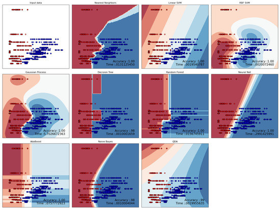
Figure 6.
Input Data () value and weight values visualization of the two classes ( Coal in blue and gangue in Red), training and testing of “Nearest Neighbors”, “Linear SVM”, “RBF SVM”, “Gaussian Process”, “Decision Tree”, “Random Forest”, “Neural Net”, “AdaBoost”, “Naive Bayes”, and “QDA” with the decision boundaries display, classification accuracy in a scale of (0–1) and time in seconds.
Table 4.
Classification Report of different classifiers trained and tested with values, values of precision, recall, F1-score, accuracy, macro avg, and weighted avg are in an average scale of (0–1), where time in seconds.
The classification report generated the precision, recall, F1-score, false prediction (F-P), macro avg, and weighted avg of every classifier training and testing, and the accuracy of the classification is driven using these factors, the support indicates the test group samples in the two classes and in total where the Time here indicates the time of classifier training and testing. It is noticeable that the training and testing using the () values achieved higher accuracy than the training with the real value, this is because the number of the training records with () is much bigger than the real values exactly 567 () values compared to 28 real values of training dataset which allow the classifiers to gain more accuracy in the classification of the classes, although the results vary because of dataset size it clearly shows the ability of the different classifiers and gives us the ability to choose between the different classifiers.
3.3. Cross Validation Test
Although the test of () values shows excellent results with the classifier test and proved that the proposed model can achieve coal gangue classification with high accuracy, this test does not show the generalization ability of the proposed model with new data, this is because the classifier training data splitting was through the whole 40 coal gangue samples which may work like a similar category where the weight values could be shared with different () values. So to strengthen the confidence in the generalization ability of the proposed model the dataset will be separated based on the different weights of the samples to test the ability of the model to classify new samples with a new weight range. The testing dataset will be chosen with samples weight within the weights range, so it should be greater than the lowest trained weight and lower than the highest trained weight to keep the range of the tested weight within the boundary of the trained category.
The samples C5 (33 3_side images), C15 (25 3_images), G6 (26 3_images), and G13 (21 3_images) were isolated from the whole dataset with a total of 105 3_images as cross-validation group to test the generalization ability, the results came with high classification accuracy vary between 96% and 100% with the different classifiers in the test Figure 7. These results indicate beyond reasonable doubt that the proposed model can perform the classification task with the new data within the same size range of the samples used in the experiment and also the ability to retrain the classifiers within a short time during the daily work in case of new sizes are noticed and retraining is needed as it is clear with the timing of the different classifiers in Table 5 that shows the timing of the training and testing of the classifiers with the total dataset.
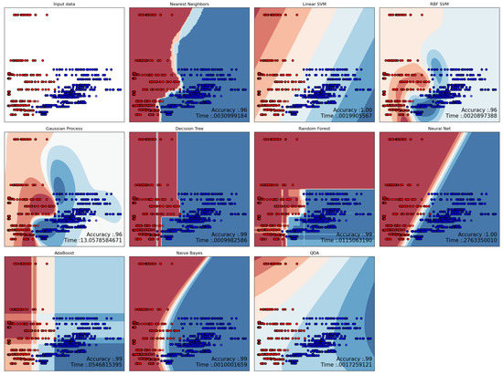
Figure 7.
value and weight values visualization of the two classes (Coal in blue and gangue in Red), Cross-validation test for “Nearest Neighbors”, “Linear SVM”, “RBF SVM”, “Gaussian Process”, “Decision Tree”, “Random Forest”, “Neural Net”, “AdaBoost”, “Naive Bayes”, and “QDA” with the decision boundaries display, classification accuracy in a scale of (0–1) and time in seconds.
Table 5.
values cross-validation test, values of precision, recall, F1-score, accuracy, macro avg, and weighted avg are in an average scale of (0–1), where time in seconds.
4. Results Discussions
Estimating the volume visual perception rather than calculating the exact volume of the objects is the technique that is presented here in this work, so making a common comparison is restricted to common factors such as classification accuracy and classification timing. The proposed work considers the hardware resources to be at the minimum level during the experiments as shown in the hardware platform details, which also drives the comparison with high structure techniques in the base of the requirement needs alongside the accuracy and timing. The increase in the accuracy results with the ExM values generated from the 3_side images increased the confidence in the efficiency of the proposed method. The results in the cross-validation test increased the confidence in the generalization ability of the model making the proposed method suitable with new data.
Table 6, shows the three steps of the experiment and the accuracy and timing to the matter of comparing the performance of the different classifiers in the classification of coal and gangue, the results show that Linear SVM classifier achieved the highest accuracy in the three steps with decent timing.
Table 6.
Sklearn classifiers accuracy with real volume values, ExM values, and Cross-Validation test.
The timing measurement with the different coal gangue classification methods differ based on the technique used where in the case of the need for preprocessing the input data to extract the needed features, this lead to extra time consumed in the image processing step such as the proposed algorithm here in this work the preprocessing step takes around 0.4 seconds with every three images of the 3_side image, comparing to the fact that with other classification methods such as the ones that use convolutional neural networks to provide the feature extraction within the structure of the network leading to reduce the execution time, Alfarzaeai et al. [2] addressed the time consumption difference between the CNN model and SVM model with feature extraction; this has been an advantage of using convolutional neural networks algorithms but in the other hand using high structure algorithms needs more resources like using YOLOv4 algorithm [25] which needs a high GPU and Memory to execute the training of the model. So the comparison bases comparing the performance of this work with previous works shall be based on the accuracy of the classification; Table 7 shows the details about some of the previous works and explains the methods applied and the accuracy of each work.
Table 7.
ExM-SVM comparing to previous work.
The works [20,24,27] used the feature extraction with SVM classifier to achieve the separation of coal and gangue, although the results were good and varied between 94% to 98.7% still the proposed work presents better accuracy with 100% this is because the difference in the extracted features, these works relied on the texture differences of the coal and gangue grayscale images which make them vulnerable to similarity and the light intensity; in the other hand, with the proposed work here, it does not trace the texture differences and rather than that it traces the volume visual perception. Also with the works that used the convolution neural networks [2,26,30] the results came with high accuracy and good timing because the use of CNN that achieve the features extraction except with [26] where they perform multispectral characteristics extraction, but the proposed work here is attracting the use of the minimum rate of requirements which is lower than using CNN requirements, also with thermal imagining the need for IR cameras and the multispectral cameras considered as high requirements which also play an important role with the efficiency of the separation, where in the proposed work the type of the used cameras is in the low range and can be used with any type of cameras. In the matter of comparing the proposed work with previous works that depend on the volume prediction as the basis of the separation process, Chen Zhang et al. [32], used a camera with a laser to predict the volume using triangular equations the results came with 60% accuracy, later in the work of W. Wang and C. Zhang [33] addressed the same technology with the use of a 3D camera but no results were presented in that paper. The work presented by Xiaojie Sun et al. [48] proposed volume prediction for coal and gangue in order to increase the efficiency of the separation process but they used only two cameras to estimate the height of the samples in order to calculate the volume, the paper did not show any results in the separation process so the comparison is insufficient also the timing of the prediction not measured.
By conducting the cross-validation test to verify the generalization ability of the proposed model, it is clear that the proposed work here achieved the highest accuracy with 100% also the timing of the proposed work came within the acceptable range with the use of the minimum operating requirements which makes it an excellent choice for coal and gangue classification tasks in real-time production lines.
5. Conclusions
The paper addressed the coal gangue classification using the density factors that stand against the harsh mining environment which affects the coal gangue classification using computer vision and presents the ExM-SVM model based on the volume visual perception and weight to classify the coal gangue in the coal mining industry. The proposed model stands in two sections, first is the feature extraction method to extract () that represents the coal gangue volume visual perception in three images to help with the irregular shape of coal and gangue, and second is the SVM classifier that performs the classification using the extracted (), and the weight of the sample.
The need for a new database of 3-side images was mandatory since the base of the work is new and there is no previous work supporting a similar dataset, so a new dataset of real coal gangue samples volume and weight values were collected alongside 3_side images of the samples, to fulfill the requirements of the proposed work. The results of the proposed model show high recognition accuracy reaching (KNN 100%, Linear SVM 100%, RBF SVM 100%, Gaussian Process 100%, Decision Tree98%, Random Forest 100%, MLP100%, AdaBosst100%, Naive Bayes 98%, and QDA 99%) and best timing with Linear SVM, cross-validation has been done to verify the generalization ability with the separated group and results also come with classification accuracy (KNN 96%, Linear SVM 100%, RBF SVM 96%, Gaussian Process 96%, Decision Tree 99%, Random Forest 99%, MLP100%, AdaBosst99%, Naive Bayes 99%, and QDA 99%) with the best timing with Decision Tree. The proposed work was tested and compared with several previous works in the matter of classification accuracy based on the timing matter and hardware requirements that support the work in real-time situations and the ability to be embedded in separation systems.
Author Contributions
Conceptualization, M.S.A.; Data curation, M.S.A. and M.M.A.A.; Formal analysis, M.S.A.; Funding acquisition, E.H. and W.P.; Investigation, M.S.A.; Methodology, M.S.A.; Project administration, E.H., W.P. and N.Q.; Resources, E.H. and W.P.; Software, M.S.A.; Supervision, E.H. and N.Q.; Validation, M.S.A.; Visualization, M.S.A.; Writing—original draft, M.S.A. and M.M.A.A.; Writing—review & editing, M.S.A. and M.M.A.A. All authors have read and agreed to the published version of the manuscript.
Funding
This work was supported by the National Natural Science Foundation of China under Grant no. 52274159.
Conflicts of Interest
The authors declare that there are no conflict of interest related to this article.
References
- International Energy Agency. Coal Information: Overview; International Energy Agency: Paris, France, 2020. [Google Scholar]
- Alfarzaeai, M.S.; Niu, Q.; Zhao, J.; Eshaq, R.M.A.; Hu, E. Coal/Gangue Recognition Using Convolutional Neural Networks and Thermal Images. IEEE Access 2020, 8, 76780–76789. [Google Scholar] [CrossRef]
- Wang, B.; Cui, C.Q.; Zhao, Y.X.; Yang, B.; Yang, Q.Z. Carbon emissions accounting for China’s coal mining sector: Invisible sources of climate change. Nat. Hazards 2019, 99, 1345–1364. [Google Scholar] [CrossRef]
- Gao, R.; Sun, Z.; Li, W.; Pei, L.; Hu, Y.; Xiao, L. Automatic Coal and Gangue Segmentation Using U-Net Based Fully Convolutional Networks. Energies 2020, 13, 829. [Google Scholar] [CrossRef]
- Wang, R.; Liang, Z. Automatic Separation System of Coal Gangue Based on DSP and Digital Image Processing. In Proceedings of the 2011 Symposium on Photonics and Optoelectronics (SOPO), Wuhan, China, 16–18 May 2011; pp. 1–3. [Google Scholar] [CrossRef]
- Hong, H.; Zheng, L.; Zhu, J.; Pan, S.; Zhou, K. Automatic Recognition of Coal and Gangue based on Convolution Neural Network. arXiv 2017, arXiv:1712.00720. [Google Scholar]
- Tripathy, D.P.; Guru Raghavendra Reddy, K. Novel Methods for Separation of Gangue from Limestone and Coal using Multispectral and Joint Color-Texture Features. J. Inst. Eng. (India) Ser. D 2017, 98, 109–117. [Google Scholar] [CrossRef]
- Xu, J.; Wang, F. Study of Automatic Separation System of Coal and Gangue by IR Image Recognition Technology. In Advances in Automation and Robotics; Lee, G., Ed.; Springer Berlin Heidelberg: Berlin/Heidelberg, Germany, 2012; Volume 2. [Google Scholar]
- Hobson, D.M.; Carter, R.M.; Yan, Y.; Lv, Z. Differentiation between Coal and Stone through Image Analysis of Texture Features. In Proceedings of the 2007 IEEE International Workshop on Imaging Systems and Techniques, Cracovia, Poland, 5 May 2007; pp. 1–4. [Google Scholar] [CrossRef]
- Su, L.; Cao, X.; Ma, H.; Li, Y. Research on Coal Gangue Identification by Using Convolutional Neural Network. In Proceedings of the 2018 2nd IEEE Advanced Information Management, Communicates, Electronic and Automation Control Conference (IMCEC), Xi’an, China, 25–27 May 2018; pp. 810–814. [Google Scholar] [CrossRef]
- Pu, Y.; Apel, D.B.; Szmigiel, A.; Chen, J. Image Recognition of Coal and Coal Gangue Using a Convolutional Neural Network and Transfer Learning. Energies 2019, 12, 1735. [Google Scholar] [CrossRef]
- Yang, D.L.; Li, J.P.; Du, C.L.; Zheng, K.H.; Liu, S.Y. Particle size distribution of coal and gangue after impact-crush separation. J. Cent. South Univ. 2017, 24, 1252–1262. [Google Scholar] [CrossRef]
- Li, J.G.; Zhan, K. Intelligent mining technology for an underground metal mine based on unmanned equipment. Engineering 2018, 4, 381–391. [Google Scholar] [CrossRef]
- Sun, Z.; Huang, L.; Jia, R. Coal and Gangue Separating Robot System Based on Computer Vision. Sensors 2021, 21, 1349. [Google Scholar] [CrossRef]
- Mu, Q.; Dong, J. The Application of Coal Cleaning Detection System Based on Embedded Real-Time Image Processing. In Proceedings of the 2013 Fifth International Conference on Measuring Technology and Mechatronics Automation, Hong Kong, China, 16–17 January 2013; pp. 1125–1127. [Google Scholar] [CrossRef]
- Li, W.; Wang, Y.; Fu, B.; Lin, Y. Coal and Coal Gangue Separation Based on Computer Vision. In Proceedings of the 2010 Fifth International Conference on Frontier of Computer Science and Technology, Changchun, China, 18–22 August 2010; pp. 467–472. [Google Scholar] [CrossRef]
- Gao, K.; Du, C.; Wang, H.; Zhang, S. An Efficient of Coal and Gangue Recognition Algorithm; Int. J. Signal Process. Image Process. Pattern Recognit. 2013, 6, 345–354. [Google Scholar]
- Sun, Z.; Lu, W.; Xuan, P.; Li, H.; Zhang, S.; Niu, S.; Jia, R. Separation of gangue from coal based on supplementary texture by morphology. Int. J. Coal Prep. Util. 2019, 42, 221–237. [Google Scholar] [CrossRef]
- He, Y.; He, J.; Zhou, N.; Chen, B.; Liang, H. Notice of Retraction: Research on identification of coal and waste rock based on PCA and GA-ANN. In Proceedings of the 2010 3rd International Conference on Computer Science and Information Technology, Chengdu, China, 9–11 July 2010; Volume 6, pp. 579–584. [Google Scholar] [CrossRef]
- Li, M.; Sun, K. An Image Recognition Approach for Coal and Gangue Used in Pick-Up Robot. In Proceedings of the 2018 IEEE International Conference on Real-time Computing and Robotics (RCAR), Kandima, Maldives, 1–5 August 2018; pp. 501–507. [Google Scholar] [CrossRef]
- Sun, J.; Su, B. Coal–rock interface detection on the basis of image texture features. Int. J. Min. Sci. Technol. 2013, 23, 681–687. [Google Scholar] [CrossRef]
- Liu, K.; Zhang, X.; Chen, Y. Extraction of Coal and Gangue Geometric Features with Multifractal Detrending Fluctuation Analysis. Appl. Sci. 2018, 8, 463. [Google Scholar] [CrossRef]
- Li, M.; Duan, Y.; He, X.; Yang, M. Image positioning and identification method and system for coal and gangue sorting robot. Int. J. Coal Prep. Util. 2020, 42, 1759–1777. [Google Scholar] [CrossRef]
- Dou, D.; Zhou, D.; Yang, J.; Zhang, Y. Coal and gangue recognition under four operating conditions by using image analysis and Relief-SVM. Int. J. Coal Prep. Util. 2018, 40, 473–482. [Google Scholar] [CrossRef]
- Liu, Q.; Li, J.; Li, Y.; Gao, M. Recognition Methods for Coal and Coal Gangue Based on Deep Learning. IEEE Access 2021, 9, 77599–77610. [Google Scholar] [CrossRef]
- Hu, F.; Zhou, M.; Dai, R.; Liu, Y. Recognition method of coal and gangue based on multispectral spectral characteristics combined with one-dimensional convolutional neural network. Front. Earth Sci. 2022, 10, 893485. [Google Scholar] [CrossRef]
- Eshaq, R.M.A.; Hu, E.; Li, M.; Alfarzaeai, M.S. Separation between Coal and Gangue based on Infrared Radiation and Visual Extraction of the YCbCr Color Space. IEEE Access 2020, 8, 55204–55220. [Google Scholar] [CrossRef]
- Li, M.; He, X.; Duan, Y.; Yang, M. Experimental study on the influence of external factors on image features of coal and gangue. Int. J. Coal Prep. Util. 2021, 42, 2770–2787. [Google Scholar] [CrossRef]
- Hu, F.; Zhou, M.; Yan, P.; Bian, K.; Dai, R. Multispectral imaging: A new solution for identification of coal and gangue. IEEE Access 2019, 7, 169697–169704. [Google Scholar] [CrossRef]
- Hu, F.; Bian, K. Accurate Identification Strategy of Coal and Gangue Using Infrared Imaging Technology Combined With Convolutional Neural Network. IEEE Access 2022, 10, 8758–8766. [Google Scholar] [CrossRef]
- Xu, B.; Liu, Q.; Ai, B.; Ding, S.; Frost, R.L. Thermal decomposition of selected coal gangue. J. Therm. Anal. Calorim. 2018, 131, 1413–1422. [Google Scholar] [CrossRef]
- Zhang, C.; Zhang, C. Coal gangue separation system based on density measurement. In Proceedings of the 2012 IEEE International Conference on Computer Science and Automation Engineering (CSAE), Zhangjiajie, China, 25–27 May 2012; Volume 1, pp. 216–218. [Google Scholar] [CrossRef]
- Wang, W.; Zhang, C. Separating coal and gangue using three-dimensional laser scanning. Int. J. Miner. Process. 2017, 169, 79–84. [Google Scholar] [CrossRef]
- Zhao, Y.D.; He, X. Recognition of coal and gangue based on X-ray. In Applied Mechanics and Materials; Trans Tech Publication: Zurich, Switzerland, 2013; Volume 275, pp. 2350–2353. [Google Scholar]
- Von Ketelhodt, L.; Bergmann, C. Dual energy X-ray transmission sorting of coal. J. S. Afr. Inst. Min. Metall. 2010, 110, 371–378. [Google Scholar]
- He, L.; Wang, S.; Guo, Y.; Hu, K.; Cheng, G.; Wang, X. Study of raw coal identification method by dual-energy X-ray and dual-view visible light imaging. Int. J. Coal Prep. Util. 2023, 43, 361–376. [Google Scholar] [CrossRef]
- Venkatesh, G.V.; Iqbal, S.M.; Gopal, A.; Ganesan, D. Estimation of Volume and Mass of Axi-Symmetric Fruits Using Image Processing Technique. Int. J. Food Prop. 2015, 18, 608–626. [Google Scholar] [CrossRef]
- Ziaratban, A.; Azadbakht, M.; Ghasemnezhad, A. Modeling of volume and surface area of apple from their geometric characteristics and artificial neural network. Int. J. Food Prop. 2017, 20, 762–768. [Google Scholar] [CrossRef]
- Soltani, M.; Omid, M.; Alimardani, R. Egg volume prediction using machine vision technique based on pappus theorem and artificial neural network. J. Food Sci. Technol. 2015, 52, 3065–3071. [Google Scholar] [CrossRef]
- Waranusast, R.; Intayod, P.; Makhod, D. Egg size classification on Android mobile devices using image processing and machine learning. In Proceedings of the 2016 Fifth ICT International Student Project Conference (ICT-ISPC), Nakhon Pathom, Thailand, 27–28 May 2016; pp. 170–173. [Google Scholar]
- Asadi, V.; Raoufat, M. Egg weight estimation by machine vision and neural network techniques (a case study fresh egg). Int. J. Nat. Eng. Sci. 2010, 4, 1–4. [Google Scholar]
- Okinda, C.; Sun, Y.; Nyalala, I.; Korohou, T.; Opiyo, S.; Wang, J.; Shen, M. Egg volume estimation based on image processing and computer vision. J. Food Eng. 2020, 283, 110041. [Google Scholar] [CrossRef]
- Anders, A.; Kaliniewicz, Z.; Markowski, P. Numerical modelling of agricultural products on the example of bean and yellow lupine seeds. Int. Agrophys. 2015, 29, 397–403. [Google Scholar] [CrossRef]
- Innocent, N.; Cedric, O.; Nyalala, L.; Makange, N.; Chao, Q.; Chao, L.; Yousaf, K.; Chen, K. Tomato volume and mass estimation using computer vision and machine learning. J. Food Eng. 2019, 263, 288–298. [Google Scholar]
- Lee, D.; Lee, K.; Kim, S.; Yang, Y. Design of an Optimum Computer Vision-Based Automatic Abalone (Haliotis discus hannai) Grading Algorithm. J. Food Sci. 2015, 80, E729–E733. [Google Scholar] [CrossRef]
- Gan, Y.; Liong, S.T.; Huang, Y.C. Automatic Surface Area and Volume Prediction on Ellipsoidal Ham using Deep Learning. arXiv 2019, arXiv:1901.04947. [Google Scholar]
- Du, C.J.; Sun, D.W. Estimating the surface area and volume of ellipsoidal ham using computer vision. J. Food Eng. 2006, 73, 260–268. [Google Scholar] [CrossRef]
- Sun, X.; Zhao, Y.; Zhao, Y. Application of Volume Detection Based on Machine Vision in Coal and Gangue Separation. In Proceedings of the 2021 IEEE 5th Conference on Energy Internet and Energy System Integration (EI2), Taiyuan, China, 22–24 October 2021; pp. 4094–4098. [Google Scholar] [CrossRef]
- Pedregosa, F.; Varoquaux, G.; Gramfort, A.; Michel, V.; Thirion, B.; Grisel, O.; Blondel, M.; Prettenhofer, P.; Weiss, R.; Dubourg, V.; et al. Scikit-learn: Machine Learning in Python. J. Mach. Learn. Res. 2011, 12, 2825–2830. [Google Scholar]
- Buitinck, L.; Louppe, G.; Blondel, M.; Pedregosa, F.; Mueller, A.; Grisel, O.; Niculae, V.; Prettenhofer, P.; Gramfort, A.; Grobler, J.; et al. API design for machine learning software: Experiences from the scikit-learn project. In Proceedings of the ECML PKDD Workshop: Languages for Data Mining and Machine Learning, Prague, Czech Republic, 23–27 September 2013; pp. 108–122. [Google Scholar]
- Canny, J.F. A Computational Approach to Edge Detection. IEEE Trans. Pattern Anal. Mach. Intell. 1986, PAMI-8, 679–698. [Google Scholar] [CrossRef]
- Van der Walt, S.; Schönberger, J.L.; Nunez-Iglesias, J.; Boulogne, F.; Warner, J.D.; Yager, N.; Gouillart, E.; Yu, T. scikit-image: Image processing in Python. PeerJ 2014, 2, e453. [Google Scholar] [CrossRef]
Disclaimer/Publisher’s Note: The statements, opinions and data contained in all publications are solely those of the individual author(s) and contributor(s) and not of MDPI and/or the editor(s). MDPI and/or the editor(s) disclaim responsibility for any injury to people or property resulting from any ideas, methods, instructions or products referred to in the content. |
© 2023 by the authors. Licensee MDPI, Basel, Switzerland. This article is an open access article distributed under the terms and conditions of the Creative Commons Attribution (CC BY) license (https://creativecommons.org/licenses/by/4.0/).