A Recursive Conic Approximation for Solving the Optimal Power Flow Problem in Bipolar Direct Current Grids

Abstract

This paper proposes a recursive conic approximation methodology to deal with the optimal power flow (OPF) problem in unbalanced bipolar DC networks. The OPF problem is formulated through a nonlinear programming (NLP) representation, where the objective function corresponds to the minimization of the expected grid power losses for a particular load scenario. The NLP formulation has a non-convex structure due to the hyperbolic equality constraints that define the current injection/absorption in the constant power terminals as a function of the powers and voltages. To obtain an approximate convex model that represents the OPF problem in bipolar asymmetric distribution networks, the conic relation associated with the product of two positive variables is applied to all nodes with constant power loads. In the case of nodes with dispersed generation, a direct replacement of the voltage variables for their expected operating point is used. An iterative solution procedure is implemented in order to minimize the error introduced by the voltage linearization in the dispersed generation sources. The 21-bus grid is employed for all numerical validations. To validate the effectiveness of the proposed conic model, the power flow problem is solved, considering that the neutral wire is floating and grounded, and obtaining the same numerical results as the traditional power flow methods (successive approximations, triangular-based, and Taylor-based approaches): expected power losses of 95.4237 and 91.2701 kW, respectively. To validate the effectiveness of the proposed convex model for solving the OPF problem, three combinatorial optimization methods are implemented: the sine-cosine algorithm (SCA), the black-hole optimizer (BHO), and the vortex search algorithm (VSA). Numerical results show that the proposed convex model finds the global optimal solution with a value of 22.985 kW, followed by the VSA with a value of 22.986 kW. At the same time, the BHO and SCA are stuck in locally optimal solutions (23.066 and 23.054 kW, respectively). All simulations were carried out in a MATLAB programming environment.

1. Introduction

Bipolar DC networks are emerging electrical systems composed of three poles, two of them with $\pm V_{DC}$ referenced to the neutral pole (third pole) [1,2]. These grids transfer two times more power than a conventional monopolar DC grid, in addition to the possibility of having special loads operated with two times the voltage, i.e., connected between the positive and negative poles [3,4,5]. Bipolar DC networks have additional advantages when compared to three-phase AC networks. The first advantage is the reduced level of energy losses, in tandem with the high quality of the voltage profiles [6]; the second advantage is the absence of reactive power and frequency variables, which allows for an easy control design, given that the only variable under control corresponds to the voltage profile at the terminals of the substation [7,8].

Figure 1 presents a comparison between the monopolar and bipolar DC configurations [9]. Figure 1a denotes a monopolar DC configuration, where it has been assumed that all the nodes with constant power terminals are solidly grounded (the most common assumption in the literature for monopolar DC configurations [10]). On the other hand, Figure 1b shows a possible configuration of constant power loads in a bipolar DC grid configuration, where the neutral wire is assumed to be solidly grounded [11]. However, for bipolar DC networks, the neutral wire can also operate under floating conduction in all the nodes except for the substation bus [12].

The main advantage of using bipolar DC configurations instead of monopolar DC topologies is that, with an additional investment in conductors (negative pole) of 33.34%, it is possible to supply more than two times the energy supplied by monopolar DC grids, with the possibility of utilizing special loads, i.e., bipolar constant power terminals [13]. However, with this advantage, analysis methodologies must also be improved to deal with bipolar DC configurations efficiently.

When analyzing bipolar DC networks under steady-state operating conditions, the power and optimal power flow problems are essential to determining their operating characteristics [13]. However, the solution to both issues requires advanced numerical methods and optimization techniques. The power flow corresponds to a feasibility problem where the main idea is to find the set of voltage values in all the poles for particular load and generation conditions. It is formulated as a set of non-affine equations, whose solution can only be reached with numerical methods [14]. On the other hand, the optimal power flow problem (OPF) is more complex, since it includes the power flow problem as a set of nonlinear constraints, and new restrictions such as the device’s capabilities and voltage regulation bounds. Furthermore, the main idea of studying the OPF is to determine the set of voltage profiles and generation inputs to minimize the total grid energy losses for particular load conditions [15]. Some recently developed approaches regarding power flow and OPF solutions are presented below.

In the case of the power flow problem, the authors of [14] presented the application of the successive approximations method to deal with the power flow solution in bipolar unbalanced DC networks with radial and meshed topologies. The main characteristic of this approach is the possibility of including the neutral wire as part of the power flow problem if it only is solidly grounded at the terminals of the substation. The study by [16] presents the application of a graph-based power flow formulation based on the upper-triangular matrix originally developed for three-phase AC grids in [17], with the aim of solving the power flow problem in bipolar unbalanced DC networks. Numerical results in the 21- and 85-bus grids demonstrated the effectiveness of the power flow problem for asymmetric bipolar DC networks. The work by [18] presents an admittance nodal formulation to address the power flow problem in bipolar DC grids while considering multiple constant power terminals. Numerical simulations in a three-bus system were implemented using PSCAD/EMTDC software. Nevertheless, the authors did not present any numerical solution method and only focused on using this software to obtain the power flow solution. In [19], a derivative-based power flow formulation based on Taylor series expansion is proposed. The authors defined this power flow formulation as the hyperbolic approximation method, as it approximates the hyperbolic relation between voltages and powers using a linear relationship. Numerical results in the 21- and 85-bus grids demonstrated this proposal’s effectiveness at dealing with the power flow solution. The authors of [20] presented the application of a fixed-point iteration method to solve the OPF problem in bipolar DC networks with multiple constant power terminals while considering current limitations in the power electronic converters that interface some of these loads. The main contribution of this work is that it demonstrates the convergence and uniqueness of the solution using the Banach fixed-point theorem. The work by [21] presents a generic power flow formulation for bipolar DC networks based on the Newton–Raphson power flow formulation. Numerical results in different test feeders demonstrate that the proposed Newton–Raphson approach allows finding the voltage profile with very close results to those provided by the PSCAD/EMTDC simulation software.

The study by [1] solved the OPF problem in highly unbalanced bipolar DC networks by applying the current injection method. The authors took into account the effect of the neutral wire in their formulation, along with the reduction of the grid congestion and the calculation of the locational marginal prices, using a linear version of the OPF problem via Taylor series. The authors of [13] presented the application of a multi-objective optimization approach to determine the optimal load balancing in bipolar DC networks with a high number of asymmetric loads. The problem was formulated as a mixed-integer linear programming model, where the constant power terminals were neglected, reducing the power flow equations to linear affine constraints. Numerical results in experimental bipolar DC networks composed of 15 and 33 nodes and multiple LED lighting systems demonstrated the effectiveness of the proposed model when compared to different combinatorial methods. In reference [22], an optimal commutation strategy to solve the optimal load-switching problem in bipolar asymmetric DC networks is proposed. The optimization problem is formulated as a mixed-integer nonlinear programming optimization problem, where DC monopolar constant power loads are interfaced with switching devices that define its connection of the positive or negative pole as a function of the energy losses and voltage behavior of the network. The proposed optimization model is solved using a genetic algorithm that defines the set of optimal load connections. Numerical simulations in MATLAB/Simulink demonstrate the effectiveness of the proposed load-switching strategy.

The work by [12] proposes the solution to the OPF problem for bipolar DC networks using a Jacobian-based formulation by applying the Newton–Raphson method. The OPF problem is formulated through a current injection power flow formulation. The authors state that the problem can be convex if the constant power loads are neglected; otherwise, the OPF becomes a nonlinear non-convex optimization problem. Numerical results in three distribution grids with multiple constant power loads confirm the effectiveness of the proposed OPF approach when compared to the solutions obtained via nonlinear solvers in commercial optimization tools. The authors of [23] presented a convex approximation method for solving the OPF problem in asymmetric bipolar DC networks. The convex equivalent model was reached by applying Taylor series expansion to the hyperbolic relation between voltages and powers at the constant power terminals. In the case of dispersed generation nodes, the hyperbolic relation between power and voltages is directly relaxed by changing the voltage variable as the value used for linearization via Taylor series expansion. Numerical results in the 21- and 33-node systems demonstrate the effectiveness of the proposed OPF solution via recursive programming when compared to three different combinatorial optimization methods.

Based on the above-presented literature review regarding the power flow and OPF solution methodologies, this research presents the following contributions:

i.

A convex approximation for the power balance constraint associated with constant power loads using a conic representation of the hyperbolic relation between voltages and currents, and a linear approximation for nodes with dispersed generation sources.

ii.

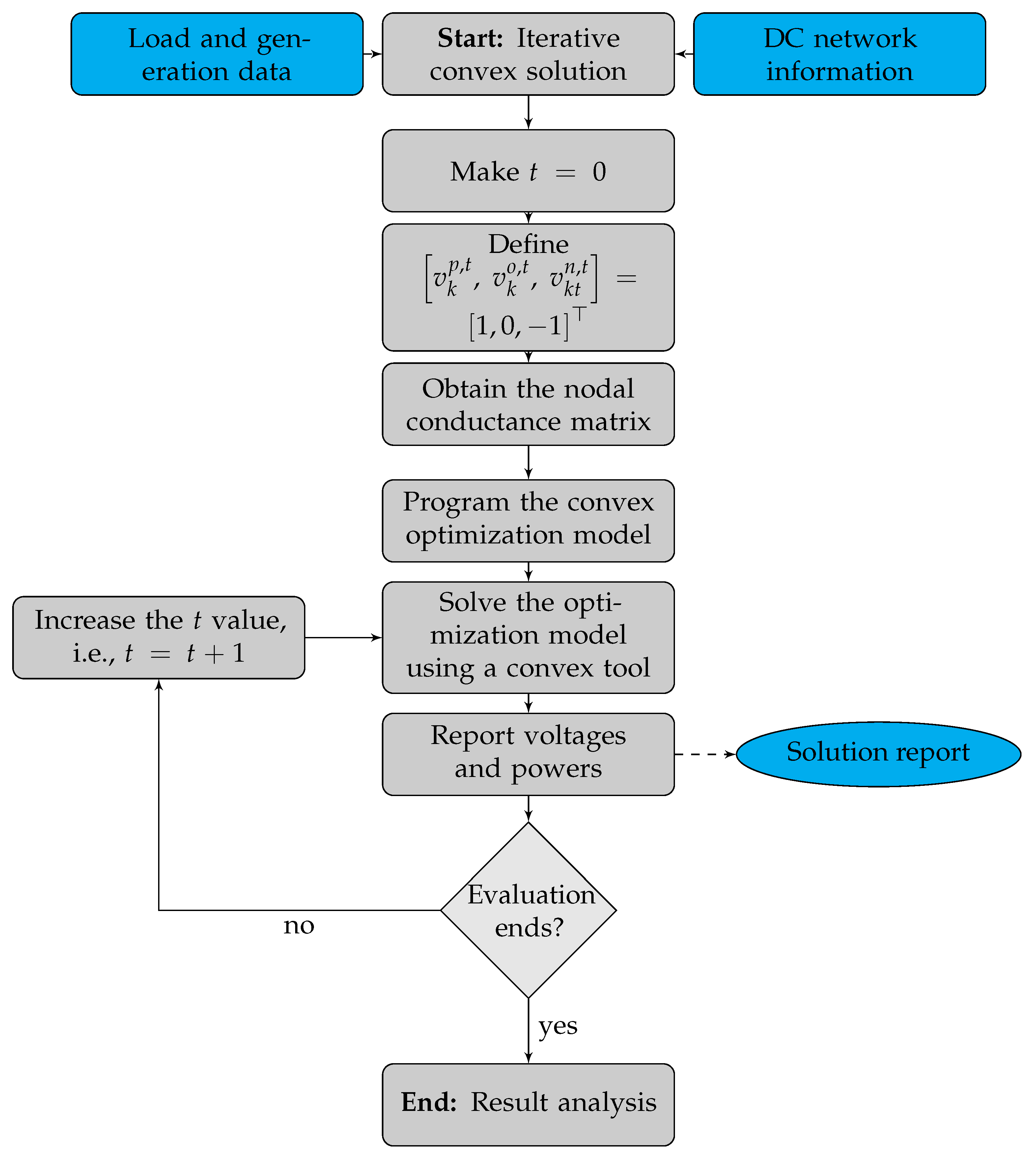
An iterative convex solution methodology to minimize the error introduced by the linear approximation of the hyperbolic relation between voltage and currents in the dispersed generation sources via recursive convex programming.

Note that the numerical results obtained in the 21-bus grid demonstrate that the proposed iterative convex solution methodology can deal with the power flow solution while considering neutral floating or solidly grounded connections with the same numerical performance as the specialized power flow approaches (successive approximations, triangular-based, and Taylor-based methodologies) [19]. In addition, a complete comparative analysis with three combinatorial optimization methods to solve the OPF problem (i.e., the sine-cosine algorithm, the black hole optimizer, and the vortex search algorithm [23]) demonstrated that the proposed iterative convex solution methodology could find the global optimal solution. In contrast, most combinatorial methods are stuck in local optima.

It is worth mentioning that in this research, the following considerations are taken into account: (i) the location and nominal capacities of the distributed generators were previously defined by the utility company; (ii) the dispersed generation sources were connected between one of the poles (positive or negative) and the neutral wire—i.e., there were no bipolar power sources; (iii) all power consumptions were modeled as constant power terminals—i.e., there were no included constant resistive or endless current loads; and (iv) the monopolar DC distribution network can be operated with the neutral wire solidly grounded at all the nodes or only at the substation bus (this case will be called the neutral floating scenario).

The remainder of this document is organized as follows. Section 2 presents the general OPF model corresponding to a nonlinear non-convex programming problem. Section 3 describes the proposed conic and linear approximations applied to the power balance constraints and the recursive approximation strategy while using an iterative solution methodology. Section 4 outlines the main characteristics of the bipolar DC version of the 21-bus grid with multiple unbalanced constant power loads. Section 5 shows the main numerical results of the proposed convex approximated solution and its detailed comparison with three different power flow methods and three combinatorial optimizers in the case of the OPF solution. Finally, Section 6 describes the conclusions and future works derived from this research.

2. Optimal Power Flow Modeling

The power flow problem in distribution networks is one of the most classical problems studied in electrical engineering [24,25]. The main idea of this problem is to set the optimal dispatch in all the distributed generators interconnected to the distribution grid in order to minimize an objective function. Typically, this objective function corresponds to the total grid power losses, i.e., the amount of power transformed into heat per unit of time in all the resistive effects of the distribution branches.

2.1. Objective Function Formulation

In the case of bipolar DC networks, this objective function can be formulated as follows:

$$\begin{array}{c}min{p}_{\mathrm{loss}}=\sum _{r\in \mathcal{P}}\sum _{j\in \mathcal{N}}{V}_j^r\left(\sum _{s\in \mathcal{P}}\sum _{k\in \mathcal{N}}{G_{jk}}^{rs}{V}_k^s\right),\end{array}$$

(1)

where $p_{\mathrm{loss}}$ denotes the objective function associated with the total grid power losses; $V_j^r$ and $V_k^s$ represent the voltage values at nodes j and k in the poles r and s, respectively; ${G_{jk}}^{rs}$ is a component of the conductance matrix G that associates nodes j and k and the poles r and s. Note that this value is different from zero if and only if nodes j and k are interconnected and r and s poles are the same. Moreover, $\mathcal{P}$ is the set that contains all the poles of the DC network (i.e., the positive, neutral, and negative ones), and $\mathcal{N}$ is the set that contains all the nodes of the bipolar DC grid under analysis.

2.2. Model Constraints

All the constraints associated with the OPF model are listed below:

$$\begin{array}{c}{I}_{g,k}^p+I_{dg,k}^p-I_{d,k}^p-I_{d,k}^{p-n}=\sum _{r\in \mathcal{P}}\sum _{j\in \mathcal{N}}{G}_{jk}^{pr}{V}_k^r,\left\{\forall k\in \mathcal{N}\right\}\end{array}$$

(2)

$$\begin{array}{c}{I}_{g,k}^o+I_{dg,k}^o-I_{d,k}^o-I_{d,k}^{\mathrm{ground}}=\sum _{r\in \mathcal{P}}\sum _{j\in \mathcal{N}}{G}_{jk}^{or}{V}_k^r,\left\{\forall k\in \mathcal{N}\right\}\end{array}$$

(3)

$$\begin{array}{c}{I}_{g,k}^n+I_{dg,k}^n-I_{d,k}^n+I_{d,k}^{p-n}=\sum _{r\in \mathcal{P}}\sum _{j\in \mathcal{N}}{G}_{jk}^{nr}{V}_k^r,\left\{\forall k\in \mathcal{N}\right\}\end{array}$$

(4)

$$\begin{array}{c}{I}_{d,k}^p=\frac{P_{d,k}^p}{V_k^p-V_k^o},\left\{\forall k\in \mathcal{N}\right\}\end{array}$$

(5)

$$\begin{array}{c}{I}_{d,k}^n=\frac{P_{d,k}^n}{V_k^n-V_k^o},\left\{\forall k\in \mathcal{N}\right\}\end{array}$$

(6)

$$\begin{array}{c}{I}_{d,k}^o=\frac{P_{d,k}^p}{V_k^o-V_k^p}+\frac{P_{d,k}^n}{V_k^o-V_k^n},\left\{\forall k\in \mathcal{N}\right\}\end{array}$$

(7)

$$\begin{array}{c}{I}_{d,k}^{p-n}=\frac{P_{d,k}^{p-n}}{V_k^p-V_k^n},\left\{\forall k\in \mathcal{N}\right\}\end{array}$$

(8)

$$\begin{array}{c}{I}_{dg,k}^p=\frac{P_{dg,k}^p}{V_k^p-V_k^o},\left\{\forall k\in \mathcal{N}\right\}\end{array}$$

(9)

$$\begin{array}{c}{I}_{dg,k}^n=\frac{P_{dg,k}^n}{V_k^n-V_k^o},\left\{\forall k\in \mathcal{N}\right\}\end{array}$$

(10)

$$\begin{array}{c}{I}_{dg,k}^o=\frac{P_{dg,k}^p}{V_k^o-V_k^p}+\frac{P_{dg,k}^n}{V_k^o-V_k^n},\left\{\forall k\in \mathcal{N}\right\}\end{array}$$

(11)

$$\begin{array}{c}{I}_{g,k}^{p,min}\le I_{g,k}^p\le I_{g,k}^{p,max},\left\{\forall k\in \mathcal{N}\right\}\end{array}$$

(12)

$$\begin{array}{c}{I}_{g,k}^{o,min}\le I_{g,k}^o\le I_{g,k}^{o,max},\left\{\forall k\in \mathcal{N}\right\}\end{array}$$

(13)

$$\begin{array}{c}{I}_{g,k}^{n,min}\le I_{g,k}^n\le I_{g,k}^{n,max},\left\{\forall k\in \mathcal{N}\right\}\end{array}$$

(14)

$$\begin{array}{c}{P}_{dg,k}^{p,min}\le P_{dg,k}^p\le P_{dg,k}^{p,max},\left\{\forall k\in \mathcal{N}\right\}\end{array}$$

(15)

$$\begin{array}{c}{P}_{dg,k}^{o,min}\le P_{dg,k}^o\le P_{dg,k}^{o,max},\left\{\forall k\in \mathcal{N}\right\}\end{array}$$

(16)

$$\begin{array}{c}{P}_{dg,k}^{n,min}\le P_{dg,k}^n\le P_{dg,k}^{n,max},\left\{\forall k\in \mathcal{N}\right\}\end{array}$$

(17)

$$\begin{array}{c}{V}^{p,min}\le V_k^p\le V^{p,max},\left\{\forall k\in \mathcal{N}\right\}\end{array}$$

(18)

$$\begin{array}{c}{V}^{n,min}\le V_k^n\le V^{n,max},\left\{\forall k\in \mathcal{N}\right\}\end{array}$$

(19)

$$\begin{array}{c}\left[\begin{array}{c}{V}_j^p\\ V_j^o\\ V_j^n\end{array}\right]=\left[\begin{array}{c}1\\ 0\\ -1\end{array}\right]V_{\mathrm{nom}},\left\{j=\mathrm{slack}\right\}\end{array}$$

(20)

where $I_{g,k}^p$, $I_{g,k}^o$, and $I_{g,k}^n$ are the current injections at node k for the positive, neutral, and negative poles by the slack source; $I_{dg,k}^p$, $I_{dg,k}^o$, and $I_{dg,k}^n$ are the current injections at node k for the positive, neutral, and negative poles by the dispersed generation sources; $I_{d,k}^p$, $I_{d,k}^o$, and $I_{d,k}^n$ are the current consumptions at node k for the positive, neutral, and negative poles; respectively; $I_{d,k}^{p-n}$ is the current consumption of a load connected between positive and negative poles; $I_{d,k}^{\mathrm{ground}}$ is the total current drained to the ground under a neutral-grounded operation scenario; $P_{d,k}^p$ and $P_{d,k}^n$ are the monopolar constant power consumptions at poles p and n with respect to the neutral pole; $P_{d,k}^{p-n}$ is the bipolar constant power consumption connected between the positive and negative poles; $V_k^p$, $V_k^o$, and $V_k^n$ are the voltage values at node k for the positive, neutral, and negative poles, respectively; $I_{g,k}^{p,min}$, $I_{g,k}^{o,min}$, and $I_{g,k}^{n,min}$ are the minimum current injections with a slack source connected at node k for the positive, neutral, and negative poles, respectively; $I_{g,k}^{p,max}$, $I_{g,k}^{o,max}$, and $I_{g,k}^{n,max}$ are the maximum current injections with a slack source connected at node k for the positive, neutral, and negative poles, respectively; $P_{g,k}^{p,min}$, $P_{g,k}^{o,min}$, $P_{g,k}^{n,min}$, $P_{g,k}^{p,max}$, $P_{g,k}^{o,max}$, and $P_{g,k}^{n,max}$ represent the minimum and maximum power injections allowed for the dispersed sources; $V^{p,min}$ and $V^{p,max}$ are the minimum and maximum voltage values allowed at node k for the positive pole; $V^{n,min}$ and $V^{n,max}$ are the minimum and maximum voltage values allowed at node k for the negative pole; and $V_{\mathrm{nom}}$ denotes the nominal voltage at the substation terminal (i.e., the slack node).

Note that the optimization model (1)–(20) that represents the problem of the OPF solution in bipolar DC networks qA originally reported in [23]. However, in order to make it suitable for solving the OPF problem while considering a floating or solidly grounded neutral wire, the following two aspects can be considered:

i.

If neutral wire is assumed to be floating, then the variable $I_{d,k}^{\mathrm{ground}}$ must be set as zero for all the nodes.

ii.

If the neutral wire is assumed to be solidly grounded at all nodes of the network, then $I_{d,k}^{\mathrm{ground}}$ is left as a free variable, and the voltage variable regarding the neutral pole (i.e., $V_k^o$) must be set as zero for all nodes of the network.

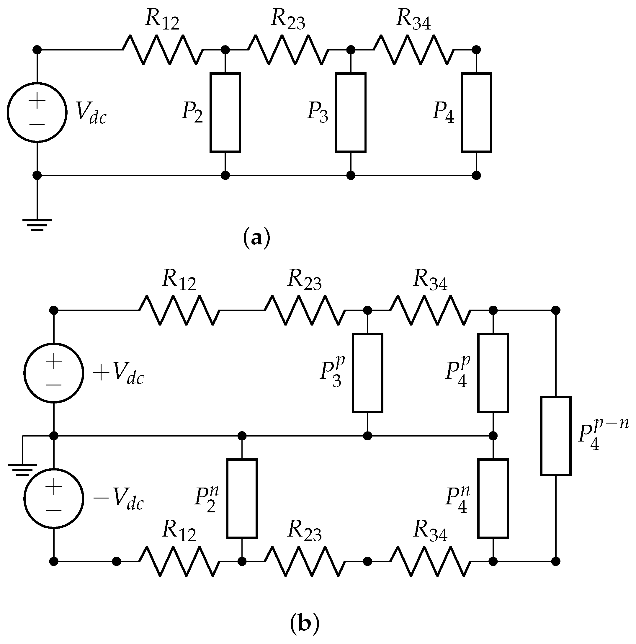
2.3. Model Interpretation

This subsection presents the complete interpretation of the OPF model, (1)–(20).

Equations (2)–(4) correspond to the current balance at each node of the network—i.e., the application of Kirchhoff’s first law using the nodal voltage method. Equations (5)–(8) define the calculation of the current demanded by a constant power terminal connected between each pair of poles. These equality constraints are obtained by applying the definition of electrical power for DC grids in the presence of constant power loads [26]. Equations (9)–(11) determine the current injections at the nodes where dispersed generators are interconnected. Box-type constraints (12)–(14) define the terminal limitations of the current outputs in the conventional generation source (i.e., the slack node). Box-type constraints (15)–(17) present the lower and upper bounds that limit power generation in dispersed sources in all the poles. Inequality constraints (18) and (19) describe the well-known voltage regulation constraints for the positive and negative poles. Finally, (20) defines the voltage output at the substation bus for each terminal; at this point, it is observed that the neutral wire is solidly grounded.

Remark 1.

By analyzing the NLP model that represents the OPF problem in unbalanced bipolar DC networks, it can be stated that (i) the objective function in (1) is convex due to the positive semi-definite nature of the conductance matrix [27]; (ii) the subset of constraints (5)–(11) shows the hyperbolic relation between voltage and power at the generation and demand nodes, being the non-convex component of the OPF problem for unbalanced bipolar DC grids.

3. Iterative Conic Solution Approach

This section presents the proposed convexification approach for the hyperbolic relations between powers and voltages in generation sources and constant power consumptions. In the case of the power generation sources, an approximation based on slight variations in the voltage profiles is considered, whereas for the constant power terminals, a conic equivalent is formulated.

3.1. A Conic Approximation for Constant Power Loads

To represent the hyperbolic relation between voltage and powers in the demand nodes, i.e., Equations (5)–(8), it is possible to obtain a conic relaxation to approximate their values as convex equivalents [28]. Let us define a generic hyperbolic function to obtain the conic equivalent representation of these currents:

$$\begin{array}{c}\hfill f\left(x,y\right)=z=\frac{C}{x-y},\end{array}$$

(21)

where C is a positive constant parameter, and x and y are two variables, such that $x-y>0$, which implies that $z>0$. From (21), it is observed that:

$$\begin{array}{cc}\hfill C& =\left(x-y\right)z,\hfill \\ \hfill C& =\frac{1}{4}{\left(z+\left(x-y\right)\right)}^2+\frac{1}{4}{\left(z-\left(x-y\right)\right)}^2,\hfill \\ \hfill 4C+{\left(z-\left(x-y\right)\right)}^2& ={\left(z+\left(x-y\right)\right)}^2,\hfill \\ \hfill {∥\begin{array}{c}2\sqrt{C}\\ x-y\end{array}∥}_2& =z+\left(x-y\right).\hfill \end{array}$$

(22)

Remark 2.

Equation (22) is entirely equivalent to the hyperbolic function (21). However, it can be relaxed as a convex constraint by changing the equal condition for a lower equal one, as proposed in [29]. This approximation is defined in Equation (23).

$$\begin{array}{c}\hfill {∥\begin{array}{c}2\sqrt{C}\\ x-y\end{array}∥}_2\le z+\left(x-y\right).\end{array}$$

(23)

If the convex relaxation is applied to constraint (5), then the following conic approximation is obtained for the current demanded at the positive pole.

$$\begin{array}{c}\hfill {∥\begin{array}{c}2\sqrt{P_{d,k}^p}\\ V_k^p-V_k^o\end{array}∥}_2\le I_{d,k}^p+\left(V_k^p-V_k^o\right),\left\{\forall k\in \mathcal{N}\right\}\end{array}$$

(24)

In the case of the current demanded at the negative pole $I_{}$, it is essential to mention that $P_{d,k}^n$ is positive. However, the denominator is negative (i.e., $V_k^n-V_k^o<0$), which implies that $I_{d,k}^n$ is also negative. In light of this, some modifications regarding the current signs can be made to the optimization model (1)–(20) in order to ensure the correct application of the conic approximation.

$$\begin{array}{c}\hfill {∥\begin{array}{c}2\sqrt{P_{d,k}^n}\\ V_k^o-V_k^n\end{array}∥}_2\le I_{d,k}^n+\left(V_k^o-V_k^n\right),\left\{\forall k\in \mathcal{N}\right\}\end{array}$$

(25)

Now, the net current injection at the neutral pole (see Equation (7)) can be rewritten as an affine equation, considering the definitions in (5) and (6):

$$\begin{array}{c}\hfill I_{d,k}^o=I_{d,k}^n-I_{d,k}^p,\left\{\forall k\in \mathcal{N}\right\}\end{array}$$

(26)

Finally, the bipolar current associated with the constant power load connected between the positive and negative poles (see Equation (8)) can be expressed as a cone approximation by using (23), as defined in (27).

$$\begin{array}{c}\hfill {∥\begin{array}{c}2\sqrt{P_{d,k}^{p-n}}\\ V_k^p-V_k^n\end{array}∥}_2\le I_{d,k}^{p-n}+\left(V_k^p-V_k^n\right),\left\{\forall k\in \mathcal{N}\right\}\end{array}$$

(27)

Remark 3.

The constraints (24)–(27) (three conic approximations and one affine constraint) allow turning the set of hyperbolic constraints (5)–(8) into a convex approximation, which constitutes the main contribution of this manuscript.

3.2. A Linear Approximation for Generation Sources

To approximate the hyperbolic relation between voltages and powers in the case of power generation sources, the following concept is taken into account. Consider a function $g\left(w,x,y\right)$ with the form defined in (28).

$$\begin{array}{c}\hfill g\left(w,x,y\right)=z=\frac{w}{x-y},\end{array}$$

(28)

where w is a positive variable in the numerator, and the denominator denotes the voltage difference between two poles, i.e., $x-y$.

Now, considering the regulatory policies for the voltage profiles and the typical operating conditions, i.e., regarding slight variations in their magnitudes with respect to their nominal rates [30], the voltage difference between these voltages can be linearized as follows:

$$\begin{array}{c}\hfill z\approx \frac{w}{x_0-y_0+{\mathsf{\Delta }}_{xy}},\end{array}$$

(29)

where if we consider that ${\mathsf{\Delta }}_{xy}$ is near zero (i.e., ${\mathsf{\Delta }}_{xy}\approx 0$), then Equation (29) takes the form shown in (30).

$$\begin{array}{c}\hfill z\approx \frac{w}{x_0-y_0},\end{array}$$

(30)

which is a linear function of the variable w, depending on the operating point assigned to the variables x and y.

Remark 4.

Considering the linear approximation in (30) for the hyperbolic Equation (28), the current injections in the dispersed generation sources (9)–(11) are approximated to linear functions (convex constraints) with the structure defined below:

$$\begin{array}{c}\hfill I_{dg,k}^{p,0}=\frac{P_{dg,k}^p}{V_k^{p,0}-V_{k,0}^{o,0}},\left\{\forall k\in \mathcal{N}\right\}\end{array}$$

(31)

$$\begin{array}{c}\hfill I_{dg,k}^{n,0}=\frac{P_{dg,k}^n}{V_k^{n,0}-V_k^{o,0}},\left\{\forall k\in \mathcal{N}\right\}\end{array}$$

(32)

$$\begin{array}{c}\hfill I_{dg,k}^{o,0}=-I_{dg,k}^{p,0}-I_{dg,k}^{n,0}.\left\{\forall k\in \mathcal{N}\right\}\end{array}$$

(33)

Observe that, with the constraints (31)–(33) and the conic approximations presented in the previous section, the OPF formulation (1)–(20) is convexified.

3.3. Approximate Convex Model and Iterative Conic Solution

For the sake of compactness, the NLP model (31)–(33) is rewritten, considering the proposed convexification methodology presented in model (34). In this model, the initial values of the voltages $\left[V_k^{p,0}{V}_k^{o,0}{V}_k^{n,0}\right]$ are redefined using the iterative counter t as $\left[V_k^{p,t}{V}_k^{o,t}{V}_k^{n,t}\right]$.

$$\begin{array}{ccc}\hfill \mathrm{Obj}.\mathrm{Func}.& min{p}_{\mathrm{loss}}=\sum _{r\in \mathcal{P}}\sum _{j\in \mathcal{N}}{V}_j^{r,t+1}\left(\sum _{s\in \mathcal{P}}\sum _{k\in \mathcal{N}}{G_{jk}}^{rs}{V}_k^{s,t+1}\right),\hfill & \hfill \\ \hfill \mathrm{Subject}\mathrm{to}.& I_{g,k}^p+I_{dg,k}^{p,t}-I_{d,k}^p-I_{d,k}^{p-n}=\sum _{r\in \mathcal{P}}\sum _{j\in \mathcal{N}}{G}_{jk}^{pr}{V}_k^{r,t+1},\hfill & \hfill \left\{\forall k\in \mathcal{N}\right\}\\ \hfill & I_{g,k}^o+I_{dg,k}^{o,t}-I_{d,k}^o-I_{d,k}^{\mathrm{ground}}=\sum _{r\in \mathcal{P}}\sum _{j\in \mathcal{N}}{G}_{jk}^{or}{V}_k^{r,t+1},\hfill & \hfill \left\{\forall k\in \mathcal{N}\right\}\\ \hfill & I_{g,k}^n+I_{dg,k}^{n,t}+I_{d,k}^n+I_{d,k}^{p-n}=\sum _{r\in \mathcal{P}}\sum _{j\in \mathcal{N}}{G}_{jk}^{nr}{V}_k^{r,t+1},\hfill & \hfill \left\{\forall k\in \mathcal{N}\right\}\\ \hfill & {∥\begin{array}{c}2\sqrt{P_{d,k}^p}\\ V_k^{p,t+1}-V_k^{o,t+1}\end{array}∥}_2\le I_{d,k}^p+\left(V_k^{p,t+1}-V_k^{o,t+1}\right),\hfill & \hfill \left\{\forall k\in \mathcal{N}\right\}\\ \hfill & {∥\begin{array}{c}2\sqrt{P_{d,k}^n}\\ V_k^{o,t+1}-V_k^{n,t+1}\end{array}∥}_2\le I_{d,k}^n+\left(V_k^{o,t+1}-V_k^{n,t+1}\right),\hfill & \hfill \left\{\forall k\in \mathcal{N}\right\}\\ \hfill & I_{d,k}^o=I_{d,k}^n-I_{d,k}^p,\hfill & \hfill \left\{\forall k\in \mathcal{N}\right\}\\ \hfill & {∥\begin{array}{c}2\sqrt{P_{d,k}^{p-n}}\\ V_k^{p,t+1}-V_k^{n,t+1}\end{array}∥}_2\le I_{d,k}^{p-n}+\left(V_k^{p,t+1}-V_k^{t+1}n\right),\hfill & \hfill \left\{\forall k\in \mathcal{N}\right\}\\ \hfill & I_{dg,k}^{p,t}=\frac{P_{dg,k}^p}{V_{k,t}^p-V_{k,t}^o},\hfill & \hfill \left\{\forall k\in \mathcal{N}\right\}\\ \hfill & I_{dg,k}^{n,t}=\frac{P_{dg,k}^n}{V_{k,t}^n-V_{k,t}^o},\hfill & \hfill \left\{\forall k\in \mathcal{N}\right\}\\ \hfill & I_{dg,k}^{o,0}=-I_{dg,k}^{p,0}-I_{dg,k}^{n,0},\hfill & \hfill \left\{\forall k\in \mathcal{N}\right\}\\ \hfill & I_{g,k}^{p,min}\le I_{g,k}^p\le I_{g,k}^{p,max},\hfill & \hfill \left\{\forall k\in \mathcal{N}\right\}\\ \hfill & I_{g,k}^{o,min}\le I_{g,k}^o\le I_{g,k}^{o,max},\hfill & \hfill \left\{\forall k\in \mathcal{N}\right\}\\ \hfill & I_{g,k}^{n,min}\le I_{g,k}^n\le I_{g,k}^{n,max},\hfill & \hfill \left\{\forall k\in \mathcal{N}\right\}\\ \hfill & P_{dg,k}^{p,min}\le P_{dg,k}^p\le P_{dg,k}^{p,max},\hfill & \hfill \left\{\forall k\in \mathcal{N}\right\}\\ \hfill & P_{dg,k}^{o,min}\le P_{dg,k}^o\le P_{dg,k}^{o,max},\hfill & \hfill \left\{\forall k\in \mathcal{N}\right\}\\ \hfill & P_{dg,k}^{n,min}\le P_{dg,k}^n\le P_{dg,k}^{n,max},\hfill & \hfill \left\{\forall k\in \mathcal{N}\right\}\\ \hfill & V^{p,min}\le V_k^{p,t+1}\le V^{p,max},\hfill & \hfill \left\{\forall k\in \mathcal{N}\right\}\\ \hfill & V^{n,min}\le V_k^{n,t+1}\le V^{n,max},\hfill & \hfill \left\{\forall k\in \mathcal{N}\right\}\\ \hfill & \left[\begin{array}{c}{V}_j^{p,t+1}\\ V_j^{o.t+1}\\ V_j^{n,t+1}\end{array}\right]=\left[\begin{array}{c}1\\ 0\\ -1\end{array}\right]V_{\mathrm{nom}},\hfill & \hfill \left\{j=\mathrm{slack}\right\}\end{array}$$

(34)

Remark 5.

The convex optimization model (34) has, as one of its main variables, the voltages at iteration $t+1$, which are a function of the voltage in the current iteration t. This implies that an iterative convex solution must be implemented in order to minimize/eliminate the error introduced by the linearization of the voltages in the power generation sources.

The iterative convex solution of the approximated model (34) that represents the OPF problem in unbalanced bipolar DC grids is illustrated in Figure 2.

It is worth mentioning that, in this research, the stopping criterion applied to determine the convergence of the optimization model (34) with the solution strategy illustrated in Figure 2 is defined as the maximum voltage magnitude difference between two consecutive iterations. This convergence criterion is presented in (34):

$$\begin{array}{c}\hfill \underset{k\in \mathcal{N},r\in \mathcal{P}}{max}\left\{\left|V_{kt+1}^r\parallel -\left|V_{kt}^r\right|\right|\right\}\le \epsilon ,\end{array}$$

(35)

where $\epsilon$ is the convergence error, assigned as $\epsilon =1\times {10}^{-8}$.

4. Test Feeder Characteristics

The 21-bus test feeder was considered in this research for all the numerical validations. It is a monopolar DC network originally reported in [31], where the convergence of the Newton–Raphson approach was demonstrated via the Kantorovich theorem.

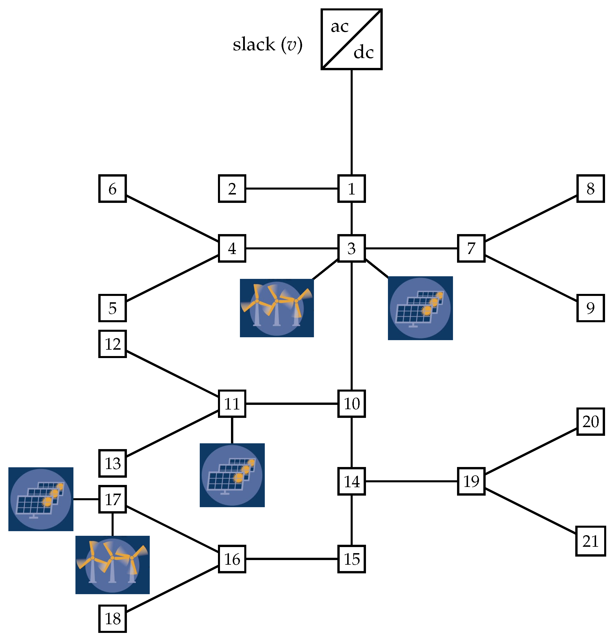
4.1. Bipolar DC Configuration

The schematic single-line diagram of the 21-bus grid is presented in Figure 3. Note that, in order to illustrate the connection of the dispersed generation sources to the positive pole in the 21-bus grid, photovoltaic generation sources are employed; and in the case of dispersed generators connected to the negative pole, wind power sources are used.

The main characteristics of this bipolar DC network (see Figure 3) are the following: (i) the substation bus operates with a voltage magnitude in the positive and negative poles of about $\pm 1000$ V, maintaining a solidly grounded neutral wire, i.e., with a voltage value equal to $0$ V; and (ii) the monopolar power consumptions (constant power loads connected between each pole and the neutral wire) for the positive and negative poles are 554 and 445 kW, respectively. In addition, the bipolar power consumption (loads connected between the positive and negative poles) is 405 kW.

4.2. Branch and Loading Information

The information regarding the distribution branches’ constant power loads and resistive values is listed in

Table 1. Data for branches and loads in the 21-bus grid (all powers in kW).

Node j	Node k	${\mathit{R}}_{\mathbf{jk}}$ ($\mathsf{\Omega }$)	${\mathit{P}}_{\mathit{d},\mathit{k}}^{\mathit{p}}$	${\mathit{P}}_{\mathit{d},\mathit{k}}^{\mathit{n}}$	${\mathit{P}}_{\mathit{d},\mathit{k}}^{\mathit{p}-\mathit{n}}$
1	2	0.053	70	100	0
1	3	0.054	0	0	0
3	4	0.054	36	40	120
4	5	0.063	4	0	0
4	6	0.051	36	0	0
3	7	0.037	0	0	0
7	8	0.079	32	50	0
7	9	0.072	80	0	100
3	10	0.053	0	10	0
10	11	0.038	45	30	0
11	12	0.079	68	70	0
11	13	0.078	10	0	75
10	14	0.083	0	0	0
14	15	0.065	22	30	0
15	16	0.064	23	10	0
16	17	0.074	43	0	60
16	18	0.081	34	60	0
14	19	0.078	9	15	0
19	20	0.084	21	10	50
19	21	0.082	21	20	0

.

4.3. Dispersed Generation Data

To assess the effectiveness of the proposed iterative convex solution for the OPF problem in unbalanced bipolar DC networks, it is considered that the 21-bus grid has four dispersed generation sources. The information on these generators is listed in

Table 2. Dispersed generation sources’ locations and capacities.

Node	Connection	Capacity (kW)
3	p	300
3	n	100
11	p	400
17	p	200
17	n	300

.

5. Computational Results

The computational implementation of the proposed iterative convex solution (ICS) was carried out in the MATLAB programming environment (version $2021b$) on a PC (64-bit version of Microsoft Windows 10 Single Language) with an AMD Ryzen 7 3700 with a $2.3$ GHz processor and 16.0 GB RAM. To solve the approximated convex model (34), a disciplined convex tool of MATLAB (CVX) was used with the SDPT3 and the SEDUMI solvers. Power flows and OPF methods were implemented with MATLAB scripts in order to compare the ICS approach.

To assess the efficiency of the ICS, two main simulations were carried out.

i.

A comparative analysis with three different power flow algorithms, two of them derivative-free and another one based on Taylor series expansion.

ii.

A comparison between the solution of the OPF problem with three combinatorial optimization methods and the proposed ICS approach.

5.1. Power Flow Solution

For comparison, three different power flow solvers are considered in order to validate the effectiveness of the proposed ICS. These are recently developed power flow methods for asymmetric bipolar DC networks, namely, (i) the successive approximations power flow (SAPF) method reported in [14], (ii) the triangular-based power flow (TBPF) approach outlined in [16], and (iii) the hyperbolic approximated power flow (HAPF) approach presented in [19].

Table 3. Power flow solution with the ICS and the comparative numerical methods.

Neutral Wire Solidly Grounded
Method	Losses (pu)	Iterations	Time (ms)
SAPF	0.954237	13	0.5275
TBPF	0.954237	13	0.8340
HAPF	0.954237	13	1.5542
ICS	0.954237	2	—
Neutral Wire Floating
Method	Losses (pu)	Iterations	Time (ms)
SAPF	0.912701	10	0.4911
TBPF	0.912701	10	0.7672
HAPF	0.912701	4	1.0212
ICS	0.912701	2	—

lists the solutions found with the proposed and comparative methods regarding the power flow problem for the 21-bus grid, considering the same convergence error and the possibility of having the neutral wire solidly grounded or floating.

The results in Table 3 show that:

i.

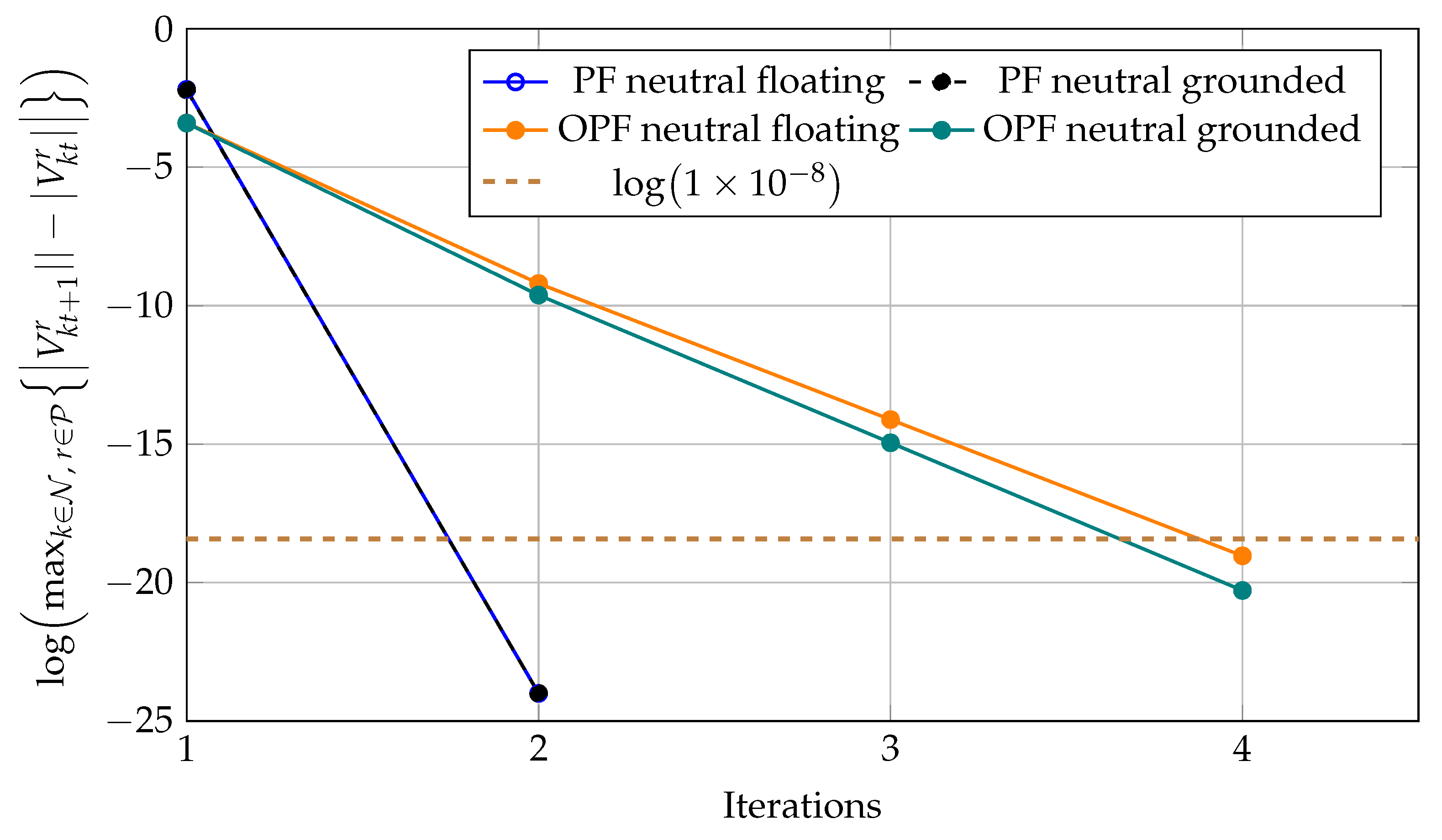
The derivative-free power flow approaches (i.e., SAPF and SAPF methods) require the same number of iterations in each simulation case. This implies that these methods are numerically equivalent for power flow studies with linear convergence. The HAPF approach for the solidly grounded case exhibited a linear convergence with the same number of iterations as the SAPF and SAPF methods; and in the case of the floating neutral wire, the convergence was quadratic, requiring four iterations, in contrast with the ten iterations taken by the SAPF and SAPF methods.

ii.

The main difference regarding the connections of the neutral wire (i.e., the solidly grounded and the floating cases) was the total grid power loss. As expected, with the floating neutral wire, the losses value was $95.4237$ kW, which was reduced to $91.2701$ kW. i.e., a variation of about $4.1536$ kW in favor of the solidly grounded connection. This is an expected behavior, as the current in the neutral wire is directly drained to the earth when it is solidly grounded, which helps to reduce power losses, in contrast with the neutral floating wire, where the presence of asymmetric loads produces neutral circulating currents.

iii.

As for processing times, the ICS takes about 5 s to solve the power flow problem, which is a higher value in comparison with the specialized power flow methods, in which only milliseconds are spent. However, it is worth highlighting that the ICS for model (34) involves an optimization problem with infinite feasible solutions and only one global optimal solution. In contrast, the specialized power flow methods can solve the problem without employing combinatorial optimization approach in a master–slave connection.

5.2. OPF Solution

In this subsection, the solution to the OPF problem is presented, which was obtained by implementing the proposed ICS methodology. Three combinatorial optimization methods were implemented for the sake of comparison, as in shown

Table 4. Selected combinatorial optimization methods.

Method	Ref.	Evaluations	Iterations	Pop. Size
Black-hole optimizer (BHO)	[32]
Sine-cosine algorithm (SCA)	[33]	100	1000	20
Vortex-search algorithm (VSA)	[34]

.

Note that the selection of the aforementioned combinatorial optimization algorithms was based on their excellent results for solving NLP problems with a non-convex structure, as was the case of model (1)–(20). In addition, 100 consecutive evaluations were performed in order to conduct a statistical analysis. Note that, in order to implement the OPF problem with metaheuristics, a master–slave optimization approach must be employed [35]. Here, the SAPF method was selected for the slave stage, in combination with each one of the algorithms in Table 4. The numerical results for the OPF problem are listed in

Table 5. Comparative analysis between combinatorial optimizers and the ICS methodology (all values in pu).

Method	Min.	Mean	Max.	Std. Dev.	Time (s)
SCA	0.23054	0.25305	0.29703	$1.39\times {10}^{-2}$	6.7870
BHO	0.23066	0.23183	0.23329	$5.90\times {10}^{-4}$	13.1513
VSA	0.22986	0.22986	0.22988	$4.23\times {10}^{-6}$	8.3176
ICS	0.22985	0.22985	0.22985	<$1\times {10}^{-16}$	11.6125

. Note that these results were obtained for the neutral wire floating, as in the scenario with the highest possible power losses.

The numerical results in Table 5 show that:

i.

The best combinatorial optimization method is the VSA, as demonstrated in [34]. This algorithm found a solution of $22.986$ kW, which is near the optimal solution reached with the ICS ($22.985$ kW). The main difference between both approaches lies in their standard deviation: the VSA reported about $4.23\times {10}^{-6}$, whereas that of the proposed ICS was less than $1\times {10}^{-16}$. These values confirm two things. (i) It is impossible to ensure 100% repeatability with the VSA approach, since the standard deviation is a measure associated with the dispersion between solutions. Even if these are in a closed ball, it is possible to obtain an answer out of it, as is the case of the maximum solution ($22.988$ kW). (ii) Due to the convex nature of the solution space in model (34), the proposed ICS always reaches the exact numerical solution, thereby confirming the standard deviation’s negligible value.

ii.

The BHO and SCA got stuck in locally optimal solutions, with values of $23.054$ and $23.066$ kW. However, these solutions can be regarded as acceptable for the power flow solution, since both were less than 0.10 kW away from the optimal one (i.e., solution found with the ICS). Nevertheless, the main problem with these solutions lies in the high variability between their minimum and maximum values, which can be observed in their standard deviation.

iii.

Concerning the processing times, it is noted that all of the OPF algorithms in Table 4 required simulation times of between 8 and 13.5 s. However, each one of the combinatorial optimizers requires multiple evaluations in order to determine their average behavior, which means that, after 100 consecutive evaluations, the processing times of the ICS were effectively 100 times higher. This implies that the proposed methodology is the most effective approach, given the fact that no statistical analysis is needed.

5.3. Complementary Analysis

To illustrate the effect of the optimal dispatch of dispersed generation sources on the electrical behavior of bipolar DC networks, this subsection presents the behavior of the voltage profiles in the benchmark case and in the case with dispersed generation and a floating neutral wire. Figure 4 presents the voltage profile at each pole for both comparison simulation cases.

The voltage behavior of the positive, neutral, and negative poles depicted in Figure 4 shows that:

i

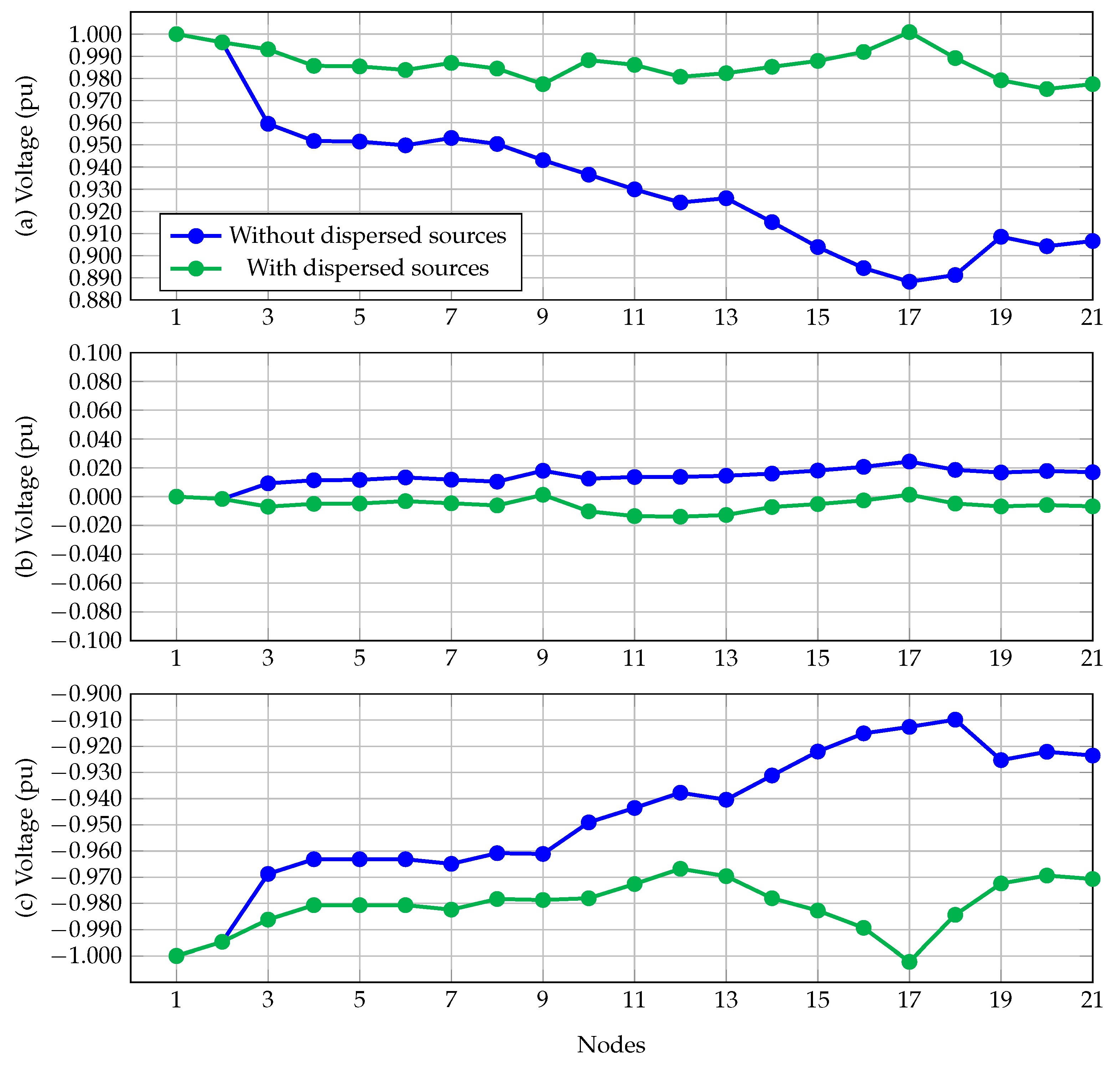
The minimum voltage in the benchmark case (without dispersed generation) occurred at the positive pole, i.e., a value of $0.8883$ pu at node 17, which implies that the voltage regulation of the bipolar DC network was about $11.17\%$. This is a significant result, as it demonstrates that, without dispersed generation, the 21-bus network does not fulfill the voltage regulation condition for distribution networks (typically $\pm 10\%$). However, this only occurs for the positive pole because it is the most loaded pole. In the case of the negative pole, the minimum voltage was $-0.9098$, which implies that the voltage regulation for this pole is below the permitted limits.

ii.

The behavior of the neutral pole shows that, once the dispersed generation is introduced into the distribution network, it helps balance the voltage behavior of the systems. Note that the maximum voltage in the neutral wire was $0.02434$ pu, i.e., 24.34 V at node 17 in the benchmark case. In contrast, when the dispersed generation was optimally dispatched, the maximum voltage deviation in the neutral wire was about $0.0139$ pu, i.e., 13.90 V at node 12.

iii.

The presence of dispersed generation in bipolar DC networks has important effects on the performance of the voltage profile. Note that node 17, for the positive and negative poles, has a magnitude of 1.0 pu, i.e., an ideal voltage profile due to the injection of power at this node with the dispersed sources. In addition, the voltage regulation for this system with dispersed sources was $3.32\%$. The minimum voltage at node 12 had a magnitude of $0.9668\mathrm{pu}$ in the negative pole.

Finally, to show the convergence of the proposed ICS in solving the power flow and OPF problems in bipolar DC networks, Figure 5 presents the convergence properties of the algorithm, considering the tolerance assigned for $\epsilon =1\times {10}^{-8}$, by plotting the following function $log\left({max}_{k\in \mathcal{N},r\in \mathcal{P}}\left\{\left|V_{kt+1}^r||-\left|V_{kt}^r\right|\right|\right\}\right)$. This function is plotted for the power flow problem and the OPF solutions reached with the proposed ICS while considering floating and neutral solidly grounded neutral connections.

Figure 5 shows that the proposed ICS methodology, which is based on the conic representation of the hyperbolic relations between voltage and powers in the constant power loads, exhibits linear convergence. In the case of the power flow, it found the optimal solution in two iterations, whereas for the OPF problem, the solution was found after four iterations. Note that, in the OPF solution, when the neutral wire was solidly grounded at each node, the final power loss was about $18.1385$ kW, which confirms that, with regard to the floating operation case, dispersed generation involves an additional reduction of about $4.8470$ kW. This result confirms that the best possible operation scenario for bipolar DC networks is when all the nodes are solidly grounded in the neutral wire, as the power losses are minimal.

6. Conclusions and Future Work

In this research, a convex approximation was implemented for the OPF problem in monopolar DC distribution networks. This convex model was obtained using two approximation concepts. The first relates to the conic equivalent representation of the product between two variables for constant power loads, and the second one is associated with the relaxation of the hyperbolic relation between voltage and powers in the dispersed generation sources, based on the slight variations in the voltages compared to the power inputs. To reduce/eliminate the error introduced by the use of the initial voltages $v_k^{p,t}$, $v_k^{o,t}$, and $v_k^{n,t}$ to determine the next set of values $v_k^{p,t+1}$, $v_k^{o,t+1}$, and $v_k^{n,t+1}$, a recursive solution approach (ICS) was implemented.

The numerical results in the 21-bus grid demonstrated that:

i.

The proposed ICS reached an equal solution for the power flow problem when compared to three different specialized power flow approaches (SAPF, TBPF, and HAPF) for both simulation cases associated with the neutral wire’s connection, i.e., the solidly grounded and floating cases.

ii.

The OPF solution showed that the ICS found the global optimal solution for the 21-bus grid, with a value of $22.985$ kW. The VSA approach, with a near-optimal solution, only followed the ICS. However, the proposed method always reached an equal optimal solution due to the convex nature of the solution space. In contrast, the VSA and the other comparison methods (BHO and SCA) can get stuck in locally optimal solutions, as evidenced by the statistical analysis.

iii.

The voltage profile analysis showed that, for the benchmark case, when the neutral wire is floating, the voltage regulation in the test feeder is about $11.17\%$. However, when the dispersed generation is optimally dispatched, the voltage regulation of the 21-bus grid is improved, with a final value of $3.32\%$. This implies that dispersed generators allow for an improvement of about $7.85\%$.

Regarding processing times, the proposed OPF approach via the ICS methodology took $11.6125$ s to solve the studied problem while a global optimum global, with the main advantage that its convergence to the solution is linear, only taking four iterations when the convergence error is set as $1\times {10}^{-8}$. At the same time, the processing times required by the other approaches oscillate between $6.7870$ and $13.15\mathrm{s}$ on average. The main problem is that a global optimum cannot be ensured. These times are also multiplied by all the evaluations required for the statistical analyses.

Possible future works derived from this work are (i) the inclusion of the optimal dispatch of renewable generation sources and batteries in the ICS approach and (ii) the implementation of the proposed convex model for solving the optimal pole-swapping problem in highly asymmetric DC networks.

References

1. Mackay, L.; Dimou, A.; Guarnotta, R.; Morales-Espania, G.; Ramirez-Elizondo, L.; Bauer, P. Optimal power flow in bipolar DC distribution grids with asymmetric loading. In Proceedings of the 2016 IEEE International Energy Conference (ENERGYCON), Leuven, Belgium, 4–8 April 2016; IEEE: Piscataway, NJ, USA, 2016. [Google Scholar] [CrossRef]
2. Monteiro, V.; Monteiro, L.F.C.; Franco, F.L.; Mandrioli, R.; Ricco, M.; Grandi, G.; Afonso, J.L. The Role of Front-End AC/DC Converters in Hybrid AC/DC Smart Homes: Analysis and Experimental Validation. Electronics 2021, 10, 2601. [Google Scholar] [CrossRef]
3. Rivera, S.; F., R.L.; Kouro, S.; Dragicevic, T.; Wu, B. Bipolar DC Power Conversion: State-of-the-Art and Emerging Technologies. IEEE J. Emerg. Sel. Top. Power Electron. 2021, 9, 1192–1204. [Google Scholar] [CrossRef]
4. Tan, L.; Zhu, N.; Wu, B. An Integrated Inductor for Eliminating Circulating Current of Parallel Three-Level DC–DC Converter-Based EV Fast Charger. IEEE Trans. Ind. Electron. 2016, 63, 1362–1371. [Google Scholar] [CrossRef]
5. Doubabi, H.; Salhi, I.; Essounbouli, N. A Novel Control Technique for Voltage Balancing in Bipolar DC Microgrids. Energies 2022, 15, 3368. [Google Scholar] [CrossRef]
6. Rivera, S.; Wu, B.; Wang, J.; Athab, H.; Kouro, S. Electric vehicle charging station using a neutral point clamped converter with bipolar DC bus and voltage balancing circuit. In Proceedings of the IECON 2013-39th Annual Conference of the IEEE Industrial Electronics Society, Vienna, Austria, 10–13 November 2013; IEEE: Piscataway, NJ, USA, 2013. [Google Scholar] [CrossRef]
7. Guo, C.; Wang, Y.; Liao, J. Coordinated Control of Voltage Balancers for the Regulation of Unbalanced Voltage in a Multi-Node Bipolar DC Distribution Network. Electronics 2022, 11, 166. [Google Scholar] [CrossRef]
8. Yang, M.; Zhang, R.; Zhou, N.; Wang, Q. Unbalanced voltage control of bipolar DC microgrid based on distributed cooperative control. In Proceedings of the 2020 15th IEEE Conference on Industrial Electronics and Applications (ICIEA), Kristiansand, Norway, 9–13 November 2020; IEEE: Piscataway, NJ, USA, 2020. [Google Scholar] [CrossRef]
9. Monteiro, V.; Oliveira, C.; Coelho, S.; Afonso, J.L. Hybrid AC/DC Electrical Power Grids in Active Buildings: A Power Electronics Perspective. In Active Building Energy Systems; Springer International Publishing: Berlin/Heidelberg, Germany, 2022; pp. 71–97. [Google Scholar] [CrossRef]
10. Li, J.; Liu, F.; Wang, Z.; Low, S.H.; Mei, S. Optimal Power Flow in Stand-Alone DC Microgrids. IEEE Trans. Power Syst. 2018, 33, 5496–5506. [Google Scholar] [CrossRef] [Green Version]
11. Kim, H.J.; Lee, Y.S.; Lee, J.G.; Han, B.M. Operation analysis of bipolar DC distribution system with voltage balancer. In Proceedings of the 2014 Australasian Universities Power Engineering Conference (AUPEC), Perth, WA, Australia, 28 September–1 October 2014; IEEE: Piscataway, NJ, USA, 2014. [Google Scholar] [CrossRef]
12. Lee, J.O.; Kim, Y.S.; Jeon, J.H. Optimal power flow for bipolar DC microgrids. Int. J. Electr. Power Energy Syst. 2022, 142, 108375. [Google Scholar] [CrossRef]
13. Chew, B.S.H.; Xu, Y.; Wu, Q. Voltage Balancing for Bipolar DC Distribution Grids: A Power Flow Based Binary Integer Multi-Objective Optimization Approach. IEEE Trans. Power Syst. 2019, 34, 28–39. [Google Scholar] [CrossRef]
14. Montoya, O.D.; Gil-González, W.; Garcés, A. A successive approximations method for power flow analysis in bipolar DC networks with asymmetric constant power terminals. Electr. Power Syst. Res. 2022, 211, 108264. [Google Scholar] [CrossRef]
15. Mackay, L.; Guarnotta, R.; Dimou, A.; Morales-Espana, G.; Ramirez-Elizondo, L.; Bauer, P. Optimal Power Flow for Unbalanced Bipolar DC Distribution Grids. IEEE Access 2018, 6, 5199–5207. [Google Scholar] [CrossRef]
16. Medina-Quesada, Á.; Montoya, O.D.; Hernández, J.C. Derivative-Free Power Flow Solution for Bipolar DC Networks with Multiple Constant Power Terminals. Sensors 2022, 22, 2914. [Google Scholar] [CrossRef]
17. Marini, A.; Mortazavi, S.; Piegari, L.; Ghazizadeh, M.S. An efficient graph-based power flow algorithm for electrical distribution systems with a comprehensive modeling of distributed generations. Electr. Power Syst. Res. 2019, 170, 229–243. [Google Scholar] [CrossRef]
18. Kim, J.; Cho, J.; Kim, H.; Cho, Y.; Lee, H. Power Flow Calculation Method of DC Distribution Network for Actual Power System. KEPCO J. Electr. Power Energy 2020, 6, 419–425. [Google Scholar] [CrossRef]
19. Sepúlveda-García, S.; Montoya, O.D.; Garcés, A. Power Flow Solution in Bipolar DC Networks Considering a Neutral Wire and Unbalanced Loads: A Hyperbolic Approximation. Algorithms 2022, 15, 341. [Google Scholar] [CrossRef]
20. Garces, A.; Montoya, O.D.; Gil-Gonzalez, W. Power Flow in Bipolar DC Distribution Networks Considering Current Limits. IEEE Trans. Power Syst. 2022, 37, 4098–4101. [Google Scholar] [CrossRef]
21. Lee, J.O.; Kim, Y.S.; Jeon, J.H. Generic power flow algorithm for bipolar DC microgrids based on Newton–Raphson method. Int. J. Electr. Power Energy Syst. 2022, 142, 108357. [Google Scholar] [CrossRef]
22. Liao, J.; Zhou, N.; Wang, Q.; Chi, Y. Load-Switching Strategy for Voltage Balancing of Bipolar DC Distribution Networks Based on Optimal Automatic Commutation Algorithm. IEEE Trans. Smart Grid 2021, 12, 2966–2979. [Google Scholar] [CrossRef]
23. Montoya, O.D.; Gil-González, W.; Hernández, J.C. Optimal Power Flow Solution for Bipolar DC Networks Using a Recursive Quadratic Approximation. Energies 2023, 16, 589. [Google Scholar] [CrossRef]
24. Balamurugan, K.; Srinivasan, D. Review of power flow studies on distribution network with distributed generation. In Proceedings of the 2011 IEEE Ninth International Conference on Power Electronics and Drive Systems, Singapore, 5–8 December 2011; IEEE: Piscataway, NJ, USA, 2011. [Google Scholar] [CrossRef]
25. Yu, D.; Cao, J.; Li, X. Review of power system linearization methods and a decoupled linear equivalent power flow model. In Proceedings of the 2018 International Conference on Electronics Technology (ICET), Chengdu, China, 23–27 May 2018; IEEE: Piscataway, NJ, USA, 2018. [Google Scholar] [CrossRef]
26. Smon, I.; Verbic, G.; Gubina, F. Local Voltage-Stability Index Using Tellegen’s Theorem. IEEE Trans. Power Syst. 2006, 21, 1267–1275. [Google Scholar] [CrossRef]
27. Garces, A. Uniqueness of the power flow solutions in low voltage direct current grids. Electr. Power Syst. Res. 2017, 151, 149–153. [Google Scholar] [CrossRef]
28. Zohrizadeh, F.; Josz, C.; Jin, M.; Madani, R.; Lavaei, J.; Sojoudi, S. A survey on conic relaxations of optimal power flow problem. Eur. J. Oper. Res. 2020, 287, 391–409. [Google Scholar] [CrossRef]
29. Farivar, M.; Low, S.H. Branch Flow Model: Relaxations and Convexification—Part I. IEEE Trans. Power Syst. 2013, 28, 2554–2564. [Google Scholar] [CrossRef]
30. Garces, A. A Linear Three-Phase Load Flow for Power Distribution Systems. IEEE Trans. Power Syst. 2016, 31, 827–828. [Google Scholar] [CrossRef]
31. Garces, A. On the Convergence of Newton’s Method in Power Flow Studies for DC Microgrids. IEEE Trans. Power Syst. 2018, 33, 5770–5777. [Google Scholar] [CrossRef]
32. Kumar, S.; Datta, D.; Singh, S.K. Black Hole Algorithm and Its Applications. In Studies in Computational Intelligence; Springer International Publishing: Berlin/Heidelberg, Germany, 2014; pp. 147–170. [Google Scholar] [CrossRef]
33. Brajević, I.; Stanimirović, P.S.; Li, S.; Cao, X.; Khan, A.T.; Kazakovtsev, L.A. Hybrid Sine Cosine Algorithm for Solving Engineering Optimization Problems. Mathematics 2022, 10, 4555. [Google Scholar] [CrossRef]
34. Doğan, B.; Ölmez, T. Vortex search algorithm for the analog active filter component selection problem. AEU-Int. J. Electron. Commun. 2015, 69, 1243–1253. [Google Scholar] [CrossRef]
35. Battarra, M.; Benedettini, S.; Roli, A. Leveraging saving-based algorithms by master–slave genetic algorithms. Eng. Appl. Artif. Intell. 2011, 24, 555–566. [Google Scholar] [CrossRef]
Figure 1. Schematic representation of monopolar and bipolar DC networks: (a) monopolar configuration and (b) bipolar configuration.
Energies 16 01729 g001
Figure 2. Proposed iterative convex solution for the approximated OPF model defined in Equation (34).
Energies 16 01729 g002
Figure 3. Single-line diagram of the 21-bus grid.
Energies 16 01729 g003
Figure 4. Voltage profile performance before and after optimally dispatching dispersed generation sources.
Energies 16 01729 g004
Figure 5. Convergence behavior of the proposed ICS methodology for the power flow and optimal power flow problems.
Energies 16 01729 g005