System Economy Improvement and Risk Shortening by Fuel Cell-UPFC Placement in a Wind-Combined System

Abstract

It is important to understand the features of an integrated renewable energy power system, especially for deregulated systems. The greatest obstacle to assimilating renewable energy generators with the existing electrical system is their unpredictability. Because wind energy is inconsistent, incorporating it into an established power system necessitates more planning. The effects of wind farm (WF) incorporation with fuel cells and a unified power flow controller (UPFC) on electric losses, voltage profile, generating price, and the economics of the system in a deregulated power market are examined in this paper. An impact analysis of integrating wind farms into controlled and uncontrolled situations is conducted. At two randomly selected locations in India, the real-time statistics of the actual wind speed (AWS) and forecasted wind speed (FWS) were merged for this study. The surplus charge rate and deficit charge rate are intended to evaluate the imbalance cost which is arising from the difference between anticipated and true wind speeds to determine the economics of the system. Customers are always trying to find electricity that is reliable, inexpensive, and efficient due to the reconfiguration of the power system. As a consequence, the security limitations of the system may be surpassed or might function beyond the safety limit, which is undesirable. In the last section, heuristic algorithms, such as sequential quadratic programming (SQP), artificial bee colony algorithms (ABC), and moth-flame optimization algorithms (MFO), are employed to analyze economic risk. In the real-time energy market, it also covers how the fuel cells and UPFC are utilized to rectify the WF integration’s deviation. Economic risk evaluation approaches include value-at-risk (VaR) and conditional value-at-risk (CVaR). A modified IEEE 30-bus test system is used throughout the whole project.

1. Introduction

The capacity to harness and utilize various sources of energy has revolutionized living conditions for people around the world since the beginning of the industrial period. Particularly, the high dependency on fossil fuels poses a major danger to the sustainability of both important human and natural systems by drastically altering the temperature of the planet [1]. Due to the introduction of new technologies that increase consumer comfort and require a lot of electrical power to function, energy demand is rising quickly nowadays. The reform of the electrical system has created intense competition among all the participants in the energy market, including retailers, transmission companies, distribution firms, and generation companies (GENCOs). It fosters an environment where clients can gain additional financial advantages [2].

However, it is exceedingly challenging to build new power stations quickly because of environmental, political, and economic hurdles. Because power supply lags behind power generation, there are several hazards associated with a competitive energy marketplace, including grid failure, severe bottleneck, financial loss to market players, etc. By optimizing the flow of electrical power, the use of renewable energy along with energy storage technologies as a power source provides a method to reduce the gap between power generation and demand.

Due to its affordability, environmental friendliness, accessibility, and independence, wind energy is among the popular renewable energy sources worldwide [3]. Electric utilities must augment their methods for maximizing the flow of power through current transmission networks due to prohibitions on the installation of new transmission lines. The most adaptable and practical alternative for regulating the flow of electricity across transmission lines is thought to be the FACTS devices. In both normal and fault scenarios, it also gives the system voltage stability [4].

Recent research has shown how fuel cells can significantly contribute to backup supply to lower system costs, have a smaller negative impact on the environment, and be less reliant on fossil fuels, while maintaining essential services. The paper [5] by Ma Zhiwen identifies methods for using fuel cells in a large network of fuel cells as distributed energy sources through nano/microgrids.

Thermal units are allowed to participate in electricity markets on most provincial power markets, and renewables are set up with independent system operators (ISO) for electricity generation priority. A two-level model of planned market allocations for electricity is proposed in this study, which considers the generation company’s bid-matching games to achieve smooth power system reform transitions [6].

A generation company’s (GenCo) profits are maximized by the profit maximization of GenCo’s shares in the electric market. Both the demand and supply sides submit bids in a regulated electricity market, and the price forecast is the benchmark for both. Bilateral agreements and energy derivatives use the long-term price estimates of electricity supply as a benchmark [7]. Conejo et al. [8] adopted the price forecast errors to account for pricing uncertainty.

A comprehensive literature review was carried out regarding deregulated electricity systems integrating renewable sources with the help of FACTS devices [9]. Ramesh et al. [10] investigated the efficiency of deregulated power systems incorporated with different energy storage techniques [10]. It is widely recognized that FACTS have a substantial influence on power transmission efficiency. The optimum placement of the distributed power flow controllers (DPFC) within a power grid should take into account operational costs and the investment of installed DPFCs [11]. Voltage and frequency fluctuations in island electrical systems are caused by fluctuations in electricity supply from renewable sources. When the power grid is shut down, the distributed generation still provides the needed electricity for that segment of the local loads [12].

Scientists published a study in Energy & Environmental Science on how to extend the life of solid oxide fuel cells, which are used to generate hydrogen and electricity [13]. In a WF-integrated power system, to reduce the system risk as well as to reduce system-generated costs, the storage systems are placed optimally within the electricity grid, applying the artificial honeybee colony (ABC) and moth-flame optimization (MFO) algorithms [14]. To address energy dispatch problems, hybrid algorithms using enhanced differential evolution (EDE) and a genetic algorithm (GA) were applied by the authors of [15]. Nature-inspired optimization algorithms include stability of frequency [16,17], cost optimization [18], energy management [19], and optimization of storage [20,21].

Although, in earlier times, various placement strategies and associated problems for WPGs, FACTS, or fuel cells, either independently or partially combining them, have been examined, no one, to the best knowledge of the authors, has tackled all these concerns concurrently. To answer these questions, which have not previously been addressed, we took all of the aforementioned factors into account.

The analysis of the literature survey indicates that studies have been conducted on various features of a deregulated system in conjunction with wind generation and energy storage systems. There were few areas to explore in this region, though the following questions were proposed: (a) From an economic and methodological perspective, what are the effects of incorporating wind power to the regulated as well as uncontrolled energy networks? (b) What relationship does the energy market’s system revenue have with imbalance costs? (c) How is the system’s profitability impacted by the disagreement between anticipated and real wind speeds? (d) In a deregulated electricity market, how does demand-side bargaining affects prices?

The present study examines all of the difficulties and places a strong emphasis on providing answers to all of these queries. The main features of this research include the following:

• This work analyzes and distinguishes regulated systems and deregulated systems where wind power is present in the system;
• A methodology is designed to investigate the implications on the power system due to the unpredictability of the wind speed with integrated wind power in a deregulated electricity scenario. If the actual and expected wind speeds diverge after the GENCOs and DISCOs form a power supply contract based on a wind speed estimate, the ISO may impose a penalty or reward the GENCOs for the excess or shortfall in power delivery. Hence, to mitigate the adverse impact of cost imbalances, GENCOs are making efforts to reduce the power gap between actual and forecast wind speeds;
• The best solution to address this shortage of power is an energy storage system. In a global energy market, storage technology systems can reduce power differences and the load on thermal power plants, allowing the financial return to be realized;
• Depending on the projected and actual wind speed for a whole day, the effect of the imbalance cost of the system on profit is discussed for two distinct sites in India;
• In this case, a fuel cell is used to deal with the adverse impact of cost imbalances in the thermal–wind–fuel cell combined system;
• To assess the efficiency of the recommended technique, SQP, ABC, and MFO are employed;
• Different optimization approaches are used here to highlight the proportional analyses of system risk before and after the deployment of fuel cells;
• The imbalance cost’s impact is evaluated. The uniqueness of this research lies in the utilization of a fuel cell to optimize profit, while reducing the impact of cost imbalances, since it has never been conducted before;
• This analysis also establishes how the location of the fuel cells and the UPFC affects the system risk profile.

2. Mathematical Modeling

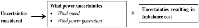
Here, considering the speed of wind at specific elevations, the generated wind power, and the cost of the wind power investment formulation, we examine the costs associated with an imbalance in a deregulated energy system.

2.1. Wind Speed Data

To begin with, two places in India (Delhi and Mumbai) were chosen to confirm the results using the data on wind speeds that have been collected. Real-time data on the actual and predicted wind speeds for the selected areas were collected at an elevation of 10 m [22,23]. To do an analysis, it is essential to determine the potential wind speed at that particular height (in India, the wind turbine hub height is 120 m). The investigation into the efficacy of the suggested strategy used the actual and predicted wind speeds, which are shown in

Table 1. FWS and AWS at 10 m elevation (in m/s).

Hour of the Day	Wind Speed of Mumbai		Wind Speed of Delhi
	Forecasted	Actual	Forecasted	Actual
1.	2.22	2.22	2.22	2.22
2.	2.22	2.50	1.67	2.22
3.	2.22	1.94	1.67	2.22
4.	2.22	2.22	1.67	2.22
5.	2.22	2.22	1.94	2.22
6.	2.22	1.94	1.94	2.22
7.	2.22	1.94	1.67	2.22
8.	2.50	2.22	1.94	2.22
9.	2.78	2.50	1.94	2.50
10.	3.06	2.50	1.67	2.50
11.	3.06	3.06	1.67	2.22
12.	3.06	3.61	1.67	2.22
13.	3.61	3.89	2.22	2.50
14.	3.89	4.17	2.50	2.50
15.	4.17	4.44	2.50	2.50
16.	4.44	4.44	2.50	2.50
17.	4.72	4.17	2.22	2.22
18.	4.44	3.33	1.94	1.94
19.	3.89	2.78	1.94	1.94
20.	3.33	2.50	1.94	1.94
21.	2.78	2.50	1.94	1.94
22.	2.50	2.22	2.22	1.94
23.	2.22	1.94	2.22	1.94
24.	1.94	1.94	2.22	2.22

.

According to the specifications, the equation of power law [24] was applied to determine the wind speed at a specified height:

$$\frac{{\mathrm{WS}}_{\mathrm{h}}}{{\mathrm{WS}}_{\mathrm{r}}}={\left(\frac{\mathrm{h}}{10}\right)}^{\mathrm{N}}$$

(1)

where ‘${\mathrm{WS}}_{\mathrm{h}}$’ = wind velocity at height ‘$\mathrm{h}$’, ‘${\mathrm{WS}}_{\mathrm{r}}$’ = reference wind velocity at a height of 10 m, and ‘$\mathrm{N}$’ = Hellman’s coefficient. h was chosen as 120 m.

2.2. Wind Power and Cost Estimation

The main factors that affect wind energy production are air density, wind speed, swept area, and the efficiency of the turbine. The wind power (WP) generated can be reflected as:

$${\mathrm{P}}_{\mathrm{w}}=\frac{1}{2}{\mathrm{D}}_{\mathrm{air}}{\mathrm{A}}_{\mathrm{t}}\mathsf{\eta }{\mathrm{WS}}_{\mathrm{h}}{}^3$$

(2)

where ‘${\mathrm{D}}_{\mathrm{air}}$’ = the air density (in kg/${\mathrm{m}}^3$), ‘${\mathrm{A}}_{\mathrm{t}}$’ = turbine’s swept area in (${\mathrm{m}}^2$), and $\mathsf{\eta }$ = the overall efficiency of the wind plant. In our work we have taken ${\mathrm{D}}_{\mathrm{air}}$ = 1.225 kg/${\mathrm{m}}^3$, $\mathsf{\eta }$ = 0.49, and the radius of the turbine rotor (r) = 40 m.

According to the wind speed data, as mentioned in Table 1, the average wind speed for all the designated sites is between 1.67 m/s and 4.72 m/s. The wind power generation costs are $3.75/MWh to invest [25]. It is anticipated that the power facility would concurrently install 50 turbines.

Table 2. Wind speed and the corresponding investment costs for wind power.

Sl. No.	Wind Velocity at 10 m (m/s)	Wind Velocity at 120 m (m/s)	Wind Power with 50 Turbines (MW)	Wind Gen Cost with 50 Turbines ($/h)	Sl. No.	Wind Speed at 10 m (m/s)	Wind Speed at 120 m (m/s)	Wind Power with 50 Turbines (MW)	Wind Gen Cost with 50 Turbines ($/h)
1	1.67	2.38	1.01	3.799	7	3.33	4.75	8.10	30.389
2	1.94	2.77	1.61	6.032	8	3.61	5.15	10.30	38.637
3	2.22	3.17	2.40	9.004	9	3.89	5.55	12.87	48.257
4	2.50	3.57	3.42	12.820	10	4.17	5.94	15.83	59.353
5	2.78	3.96	4.69	17.586	11	4.44	6.34	19.21	72.033
6	3.06	4.36	6.24	23.407	12	4.72	6.73	23.04	86.401

summarizes the speed of the wind at the necessary height, the amount of energy that can be generated from the wind, and the wind cost associated with various wind speeds.

To increase economic profits by combining wind power stations with UPFCs in a competitive double-auction power market, a UPFC static model has been employed in this study.

2.3. UPFC Static Model

A UPFC is the FACTS component with the widest range of applications for controlling voltage and power flow in transmission lines. It may alter the series injected voltage’s amplitude and phase angle simultaneously or individually, as well as the reactive current drawn by the shunt-coupled voltage source converter. By adjusting the transmission line’s series reactance together with shunt-connected reactive power injections or extractions on the associated bus, the UPFC may be used as either a capacitive or an inductive compensation, respectively. Here, a DC link connects two voltage source converters that are coupled together to form a UPFC. Figure 1 depicts the transmission line architecture with the UPFC static model where a specific UPFC is linked between buses i and j.

The UPFC’s reactance is influenced by the reactance of the transmission line where it will be placed:

$${\mathrm{X}}_{\mathrm{L}}={ \mathrm{X}}_{\mathrm{i}-\mathrm{j}}+{ \mathrm{X}}_{\mathrm{upfc}}$$

(3)

where

$${\mathrm{X}}_{\mathrm{upfc}}= \mathrm{UPFC}’\mathrm{s} \mathrm{series} \mathrm{converter}’\mathrm{s} \mathrm{reactance}={\mathrm{X}}_{\mathrm{L}}\times {\mathrm{k}}_{\mathrm{upfc}}$$

(4)

${\mathrm{X}}_{\mathrm{L}}$ = total line reactance between bus i and j (at the location of the UPFC).

The UPFC compensation level’s range is considered as [26,27] $-0.7\le {\mathrm{k}}_{\mathrm{upfc}}\le 0.2.$ Because 100% compensation will cause a resonance issue in the series circuit of the system, the safe limit of the reactance of the line is considered as 70% for compensation. According to the model, as it is presented, the Q_upfc delivers or drains reactive power through a shunt converter at the line’s designated bus, which is where the UPFC is situated.

2.4. Investment Cost of the UPFC

Due to the substantial capital costs of UPFC devices, a cost optimization approach for their deployment is crucial. The employed UPFC investment cost models were inspired by [28,29,30,31,32,33,34,35]. In this study, the UPFC device’s lifespan (LS) and rate of interest (I_r) are considered to be 0.05 and 15 years, respectively. The following formula has been utilized to calculate the UPFC’s investment cost:

$${\mathrm{IC}}_{\mathrm{upfc}}=0.0003{\mathrm{S}}_{\mathrm{oz}}^2-0.2691{\mathrm{S}}_{\mathrm{oz}}+188.22 \$/\mathrm{kVar}$$

(5)

where

$${\mathrm{S}}_{\mathrm{oz}}=\mathrm{operating} \mathrm{zone} \mathrm{or} \mathrm{range} \mathrm{of} \mathrm{UPFC}=\left|{\mathrm{Q}}_{\mathrm{x}}\right|-\left|{\mathrm{Q}}_{\mathrm{y}}\right| \mathrm{MVar}$$

(6)

${\mathrm{Q}}_{\mathrm{x}}= \mathrm{flow} \mathrm{of}$ reactive power in the line post-UPFC installation, and ${\mathrm{Q}}_{\mathrm{y}}= \mathrm{flow} \mathrm{of}$ reactive power in the line before UPFC installation.

The total investment cost for UPFC devices is computed as:

$$\mathrm{T}\_{\mathrm{IC}}_{\mathrm{upfc}}=({\mathrm{IC}}_{\mathrm{upfc}}\times {\mathrm{S}}_{\mathrm{oz}}\times 1000) \$$$

(7)

Due to UPFC devices’ high cost, a cost assessment is required to find out if a new UPFC device is the most cost-effective option among potential installation locations. In this regard, the investment cost is transformed into a per-year value using the following equation:

$$\mathrm{AT}\_{\mathrm{IC}}_{\mathrm{upfc}}=\mathrm{T}\_{\mathrm{IC}}_{\mathrm{upfc}}\frac{{\mathrm{I}}_{\mathrm{r}}{\left(1+{\mathrm{I}}_{\mathrm{r}}\right)}^{\mathrm{LS}}}{{\left(1+{\mathrm{I}}_{\mathrm{r}}\right)}^{\mathrm{LS}}-1}\$$$

(8)

where $\mathrm{AT}\_{\mathrm{IC}}_{\mathrm{upfc}}$ = annual UPFC investment cost considering all the factors mentioned above.

2.5. Fuel Cell Model

An electrolyzer employs the reverse reaction to electrolyze water to produce hydrogen; while using hydrogen as fuel, a fuel cell turns the chemical energy into electrical energy. Together, these components make up the storage system. The following equation shows the reversible chemical interaction between oxygen and hydrogen, which results in the production of electrical energy, heat, and water.

$$2{\mathrm{H}}_2+{\mathrm{O}}_2\to {\mathrm{H}}_2\mathrm{O}+\mathrm{Electrical} \mathrm{Energy}+\mathrm{Heat}$$

(9)

In tanks, the generated hydrogen is kept, enabling the utilization of the gas for both short- and long-term storage. In comparison to large-scale storage systems such as batteries or pumped hydro storage, the efficiency of hydrogen storage is quite high [36]. The storage system operates according to the following principle:

2.5.1. Low-Demand Period (The Electrolyzer Produces Hydrogen to Be Stored in Tanks)

The consumed energy by the electrolyzer is represented as:

$${\mathrm{E}}_{\mathrm{elz}}=\frac{{\mathrm{hv}}_{{\mathrm{H}}_2}^{\mathrm{l}}\times {\mathrm{E}}_{{\mathrm{H}}_2}^{\mathrm{p}}}{{\mathsf{\eta }}_{\mathrm{elz}}}$$

(10)

where ${\mathrm{E}}_{{\mathrm{H}}_2}^{\mathrm{p}}=\mathrm{hydrogen} \mathrm{produced} \mathrm{by} \mathrm{the} \mathrm{electrolyzer};$

${\mathrm{E}}_{\mathrm{elz}}=\mathrm{energy} \mathrm{consumed} \mathrm{by} \mathrm{the} \mathrm{electrolyzer};$

${\mathsf{\eta }}_{\mathrm{elz}}=\mathrm{efficiency} \mathrm{of} \mathrm{the} \mathrm{electrolyzer}$;

${\mathrm{hv}}_{{\mathrm{H}}_2}^{\mathrm{l}}=\mathrm{lower} \mathrm{heating} \mathrm{value} \mathrm{of} \mathrm{hydrogen}.$

2.5.2. High-Demand Period (Stored Hydrogen to Be Used in the Fuel Cell to Supply the Demand)

The fuel cell produces electricity using hydrogen during peak hours, and the power-producing capacity is directly related to the use of hydrogen.

$${\mathrm{E}}_{\mathrm{fc}}={\mathsf{\eta }}_{\mathrm{fc}}\times {\mathrm{fc}}_{{\mathrm{H}}_2}^{\mathrm{con}}\times {\mathrm{hv}}_{{\mathrm{H}}_2}^{\mathrm{l}}$$

(11)

where

${\mathrm{E}}_{\mathrm{fc}}=\mathrm{energy} \mathrm{produced} \mathrm{from} \mathrm{the} \mathrm{fuel} \mathrm{cell};$

${\mathrm{fc}}_{{\mathrm{H}}_2}^{\mathrm{con}}=\mathrm{hydrogen} \mathrm{consumption} \mathrm{in} \mathrm{the} \mathrm{fuel} \mathrm{cell};$

${\mathsf{\eta }}_{\mathrm{fc}}=\mathrm{efficiency} \mathrm{of} \mathrm{the} \mathrm{fuel} \mathrm{cell}.$

2.6. Social Welfare (SW) and Locational Marginal Pricing (LMP)

The mismatch between society’s acceptance of paying for its need for energy and the expense of providing that demand is known as social welfare. The cost and supply of power for a certain provider ‘i’ is expressed as [37]:

$${\mathrm{P}}_{\mathrm{i}}={\mathrm{RP}}_{\mathrm{i}}+{\mathrm{m}}_{\mathrm{G}}{\mathrm{P}}_{\mathrm{G}\left(\mathrm{i}\right)}$$

(12)

where ${\mathrm{P}}_{\mathrm{i}}$ = the cost that ‘i’ is ready to provide ($/MWh);

${\mathrm{RP}}_{\mathrm{i}}$ = the intercept (reservation price ${\mathrm{RP}}_{\mathrm{i}}>0$);

${\mathrm{m}}_{\mathrm{G}}$ = the slope of the generation ($>0$) ($/MW²h);

${\mathrm{P}}_{\mathrm{G}\left(\mathrm{i}\right)}$ = supply (MW);

N_g = number of generation buses.

At the operational point (P_i, G_i), the apparent cost of production is expressed as:

$$\mathrm{C}{\left(\mathrm{i}\right)}_{{\mathrm{P}}_{\mathrm{G}\left(\mathrm{i}\right)}}={\mathrm{RP}}_{\mathrm{i}}\times {\mathrm{P}}_{\mathrm{G}\left(\mathrm{i}\right)}+\frac{1}{2}{\mathrm{m}}_{\mathrm{G}}{\mathrm{P}}_{\mathrm{G}\left(\mathrm{i}\right)}^2$$

(13)

Likewise, the linear demand curve for the customer ‘j’ is expressed by:

$${\mathrm{P}}_{\mathrm{j}}={\mathrm{RP}}_{\mathrm{j}}+{\mathrm{m}}_{\mathrm{D}}{\mathrm{P}}_{\mathrm{D}\left(\mathrm{j}\right)}$$

(14)

where ${\mathrm{P}}_{\mathrm{j}}$ = the cost that ‘j’ is ready to pay ($/MWh);

${\mathrm{RP}}_{\mathrm{j}}$ = the intercept (reservation price ${\mathrm{RP}}_{\mathrm{j}}>0$);

${\mathrm{m}}_{\mathrm{D}}$ = the slope ($/MW²h);

${\mathrm{P}}_{\mathrm{D}\left(\mathrm{j}\right)}$ = demand supply (MW);

N_d = number of demand buses.

The consumer benefit can be presented as:

$$\mathrm{B}{\left(\mathrm{j}\right)}_{{\mathrm{P}}_{\mathrm{D}\left(\mathrm{j}\right)}}={\mathrm{RP}}_{\mathrm{j}}\times {\mathrm{P}}_{\mathrm{D}\left(\mathrm{j}\right)}+\frac{1}{2}{\mathrm{m}}_{\mathrm{D}}{\mathrm{P}}_{\mathrm{D}\left(\mathrm{j}\right)}^2$$

(15)

Therefore, social welfare is interpreted as:

$$\mathrm{SW}={{\displaystyle \sum }}_{\mathrm{j}=1}^{{\mathrm{N}}_{\mathrm{d}}}\mathrm{B}{\left(\mathrm{j}\right)}_{{\mathrm{P}}_{\mathrm{D}\left(\mathrm{j}\right)}}-{{\displaystyle \sum }}_{\mathrm{i}=1}^{{\mathrm{N}}_{\mathrm{g}}}\mathrm{C}{\left(\mathrm{i}\right)}_{{\mathrm{P}}_{\mathrm{G}\left(\mathrm{i}\right)}}$$

(16)

It is revealed from Equation (16) that social welfare is the union of the generating cost of electricity and consumer benefits. Hence, to optimize social welfare, customer benefits must be maximized while minimizing power-generating costs. The maximizing of SW in this study is obtained by minimizing the objective function, as demonstrated in Equation (35) [38].

Locational marginal pricing is a very important part of mathematical modeling and is also termed nodal pricing (NP). This technique of setting pricing involves figuring out market-clearing prices at various transmission grid nodes or locations. It is constituted of the total of the marginal costs of transmission congestion, losses, and generation.

LMP = Marginal cost of (congestion in transmission + losses + generation)

(17)

2.7. Risk Assessment

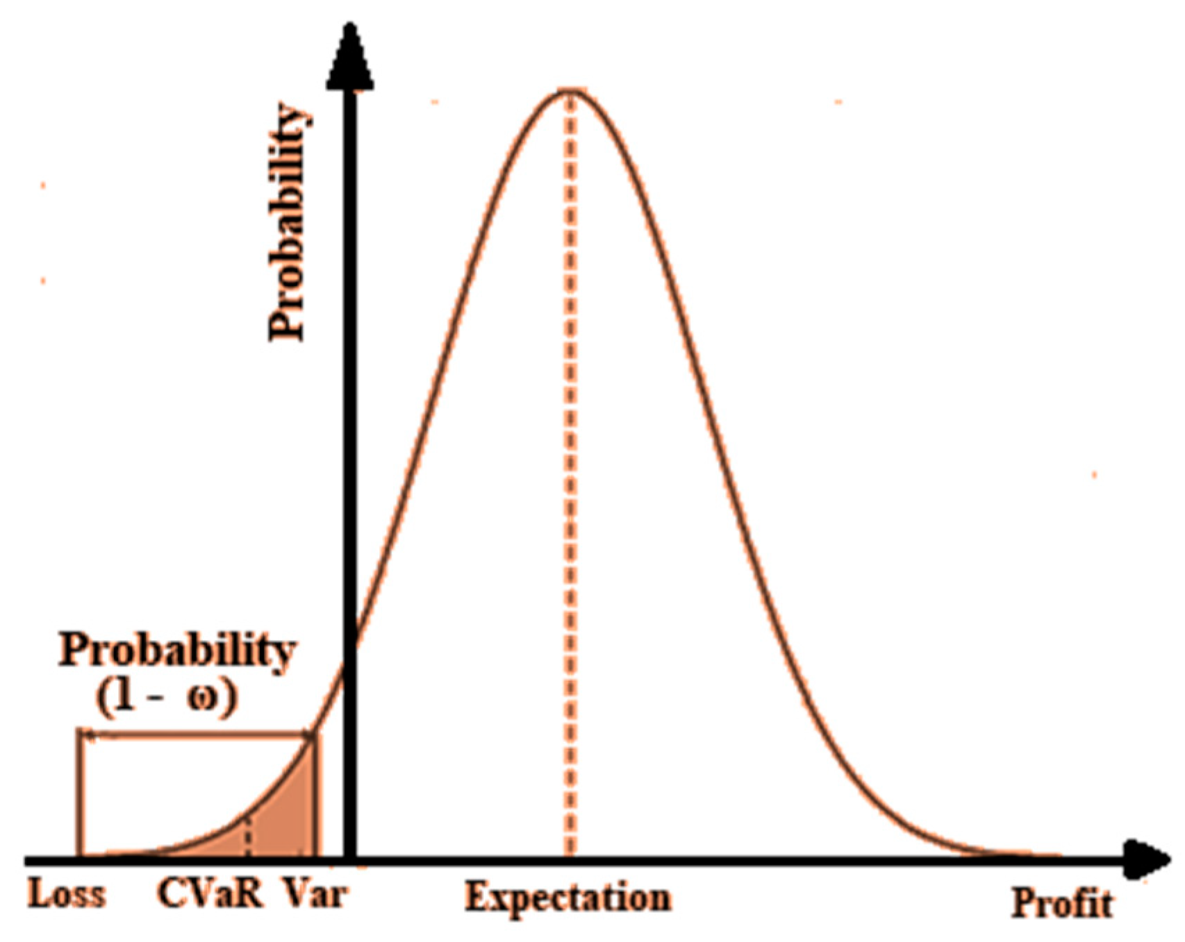
In today’s competitive environment, the necessity for risk assessment and management is becoming more and more crucial. In the realm of risk management, the approaches of value-at-risk (VaR) and conditional value-at-risk (CVaR) have grown in popularity. Based on probabilistic research and assurance confidence levels, both evaluation methods are built. VaR determines the maximum loss and level of confidence for a given period. CVaR is the most precise risk-measuring technique for calculating the potential loss in tail events since VaR does not reflect the amount of loss that may occur over the threshold. For instance, if VaR is estimated at a 95% confidence level, CVaR may be calculated considering the average of the 5% worst losses. The additional losses in the remaining 5% make up the CVaR. With a loss amount of (1 − ω) percentile, VaR thus denotes the lowest loss, whereas CVaR gives the average loss components in the lower end of the loss distribution.

Here, g(x,y) is the loss related to the decision vector Q, which is to be chosen from a specific subset x of $\dot{\mathrm{R}}$ and the random vector y in $\dot{\mathrm{R}}$. ‘ω’ is the confidence level. The possibility that g(x,y) does not exceed a threshold ζ is represented by p(y) and is thus expressed as [39]:

$$\mathsf{\psi }\left(\mathrm{x},\mathsf{\zeta }\right)={{\displaystyle \int }}_{\mathrm{g}\left(\mathrm{x},\mathrm{y}\right)\le \mathsf{\zeta }}\mathrm{p}\left(\mathrm{y}\right)\mathrm{dy}$$

(18)

Mathematically, the assurance level based on VaR and CVaR is represented by:

$${\mathsf{\zeta }}_{\mathsf{\omega }}\left(\mathrm{x}\right)=\min \left\{\mathsf{\zeta }\in \dot{\mathrm{R}}:\mathsf{\psi }\left(\mathrm{x},\mathsf{\zeta }\right)\right\}$$

(19)

$${\mathsf{\phi }}_{\mathsf{\omega }}\left(\mathrm{x}\right)=\frac{1}{1-\mathsf{\omega }}\left[\left({{\displaystyle \sum }}_{\mathrm{j}=1}^{{\mathrm{j}}_{\mathsf{\omega }}}{\mathrm{p}}_{\mathrm{j}}-\mathsf{\omega }\right){\mathrm{a}}_{{\mathrm{j}}_{\mathsf{\omega }}}+{{\displaystyle \sum }}_{\mathrm{j}={\mathrm{j}}_{\mathsf{\omega }}}^{\mathrm{T}}{\mathrm{p}}_{\mathrm{j}}{\mathrm{a}}_{\mathrm{j}}\right]$$

(20)

where T = the quantity of attempts conducted under various circumstances, and loss points are arranged as: ${\mathrm{a}}_1<{\mathrm{a}}_2<{\mathrm{a}}_3\dots \dots <{\mathrm{a}}_{\mathrm{T}}$.

3. Objective Function

Let us consider an electricity network with ‘N_b’ buses, ‘N_g’ generators, and ‘N_l’ loads. Mathematically, the proposed approach’s primary goals are to maximize societal welfare, reduce system generating costs, optimize investment costs for the UPFC, and limit investment costs for wind power generation. This research aims to increase social good and commercial gain while reducing generation costs and system risk in the case of cost imbalances. For the performance study of any renewable integrated power system, the imbalance cost concept must be taken. However, to the authors’ knowledge, only a few researchers have taken this idea. The system operators use rewards and penalties to create revenue; thus, the positive imbalance cost increases the system profit, while the negative imbalance cost decreases it. The maximization and minimization problems are the two objective functions in this study, respectively. The objective functions are modeled mathematically as:

3.1. The Objective Function (First Part)

P_n(t) = TR_n(t) + IMC_n(t) − TGC_n(t)

(21)

where P_n(t) = the n-th unit’s total profit at a time ‘t’, TR_n(t) = total revenue, IMC_n(t) = total imbalance cost, and TGC_n(t) = overall generation cost (containing the investment costs for wind power generation and thermal power generation).

The most crucial element in optimizing the profit of wind–thermal power plants under the newly deregulated electricity environment is the imbalance cost, which is the most significant consideration among the revenue, imbalance cost, and overall generating cost. The following is a description of the formulae for the total income, imbalance cost, and generation cost:

$${\mathrm{TR}}_{\mathrm{n}\left(\mathrm{t}\right)}={{\displaystyle \sum }}_{\mathrm{i}=1}^{{\mathrm{N}}_{\mathrm{g}}}{\mathrm{P}}_{\mathrm{a},\mathrm{i}\left(\mathrm{t}\right)}.{\mathrm{LMP}}_{\mathrm{i}\left(\mathrm{t}\right)}$$

(22)

$${\mathrm{IMC}}_{\mathrm{m}\left(\mathrm{t}\right)}={{\displaystyle \sum }}_{\mathrm{i}=1}^{{\mathrm{N}}_{\mathrm{g}}}\left[{\mathrm{CR}}_{\mathrm{s}\left(\mathrm{t}\right)}+{ \mathrm{CR}}_{\mathrm{d}\left(\mathrm{t}\right)}.{\left(\frac{{\mathrm{P}}_{\mathrm{f},\mathrm{i}\left(\mathrm{t}\right)}}{{\mathrm{P}}_{\mathrm{a},\mathrm{i}\left(\mathrm{t}\right)}}\right)}^2\right].\left[{\mathrm{P}}_{\mathrm{a},\mathrm{i}\left(\mathrm{t}\right)}-{ \mathrm{P}}_{\mathrm{f},\mathrm{i}\left(\mathrm{t}\right)}\right]$$

(23)

where ${\mathrm{P}}_{\mathrm{a},\mathrm{i}\left(\mathrm{t}\right)}$ = power generated with actual wind speed at a time ‘t’ at thr i-th generation bus, ${\mathrm{P}}_{\mathrm{f},\mathrm{i}\left(\mathrm{t}\right)}$ = power generated with the forecasted wind speed, ${\mathrm{CR}}_{\mathrm{s}\left(\mathrm{t}\right)}$ = charge rate (surplus), and ${\mathrm{CR}}_{\mathrm{d}\left(\mathrm{t}\right)}$ = charge rate (deficit).

TGC_m(t) = GC_m(t) + WGC_m(t) + Cost_upfc

(24)

where WGC = wind power investment cost. In a wind-incorporated deregulated setup, the wind-generated electricity is committed after being calculated based on the anticipated wind speed. If the actual wind speed data turns out to be different from the forecasted one, the fuel cell can aid to lessen the power required for operation to make up for the discrepancy. However, there may be expenditures associated with the imbalance caused by the discrepancy between the projected and actual wind speeds. Equation (23) shows the imbalance cost. The calculation methods for the charge rates (deficit and excess) are as follows:

$${\mathrm{CR}}_{\mathrm{d}\left(\mathrm{t}\right)}=\left(1+\mathsf{\gamma }\right).{ \mathrm{LMP}}_{\mathrm{i}\left(\mathrm{t}\right)},{ \mathrm{CR}}_{\mathrm{s}\left(\mathrm{t}\right)}=0{ \mathrm{when} \mathrm{P}}_{\mathrm{a},\mathrm{i}\left(\mathrm{t}\right)}<{\mathrm{P}}_{\mathrm{f},\mathrm{i}\left(\mathrm{t}\right)}$$

(25)

$${\mathrm{CR}}_{\mathrm{s}}\left(\mathrm{t}\right)=\left(1-\mathsf{\gamma }\right).{ \mathrm{LMP}}_{\mathrm{i}}\left(\mathrm{t}\right),{ \mathrm{CR}}_{\mathrm{d}}\left(\mathrm{t}\right)=0{ \mathrm{when} \mathrm{P}}_{\mathrm{a},\mathrm{i}\left(\mathrm{t}\right)}>{\mathrm{P}}_{\mathrm{f},\mathrm{i}\left(\mathrm{t}\right)}$$

(26)

$${\mathrm{CR}}_{\mathrm{s}}\left(\mathrm{t}\right)={\mathrm{CR}}_{\mathrm{d}}\left(\mathrm{t}\right){ \mathrm{when} \mathrm{P}}_{\mathrm{a},\mathrm{i}\left(\mathrm{t}\right)}={ \mathrm{P}}_{\mathrm{f},\mathrm{i}\left(\mathrm{t}\right)}$$

(27)

$${\mathrm{GC}}_{\mathrm{m}\left(\mathrm{t}\right)}={{\displaystyle \sum }}_{\mathrm{i}=1}^{{\mathrm{N}}_{\mathrm{g}}}\mathrm{x}+\mathrm{y}.{\mathrm{P}}_{\mathrm{a},\mathrm{i}\left(\mathrm{t}\right)}+\mathrm{z}.{\mathrm{P}}_{\mathrm{a},\mathrm{i}\left(\mathrm{t}\right)}{}^2$$

(28)

where ${\mathrm{LMP}}_{\mathrm{i}\left(\mathrm{t}\right)}$ = LMP at time ‘t’ at the i-th bus, ${\mathrm{GC}}_{\mathrm{m}\left(\mathrm{t}\right)}=$ power generation cost of the thermal unit, and X, y, and z are coefficients of the generation cost. The ICR, or imbalance charge rate (surplus or deficit), to MCP ratio is used to indicate the imbalance cost coefficient or ‘$\mathsf{\gamma }$’. In the present work, the value of ‘$\mathsf{\gamma }$’ is considered as 0.9.

3.2. The Objective Function (Second Part)

$$\mathrm{Min}.{ \mathsf{\zeta }}_{\mathsf{\omega }}\left(\mathrm{x}\right)=\min \left\{\mathsf{\zeta }\in \dot{\mathrm{R}}:\mathsf{\psi }\left(\mathrm{x},\mathsf{\zeta }\right)\right\}$$

(29)

$$\mathrm{Min}.{ \mathsf{\phi }}_{\mathsf{\omega }}\left(\mathrm{x}\right)=\frac{1}{1-\mathsf{\omega }}\left[\left({{\displaystyle \sum }}_{\mathrm{j}=1}^{{\mathrm{j}}_{\left(\mathsf{\omega }\right)}}{\mathrm{p}}_{\mathrm{j}}-\mathsf{\omega }\right){\mathrm{a}}_{{\mathrm{j}}_{\left(\mathsf{\omega }\right)}}+{{\displaystyle \sum }}_{\mathrm{j}={\mathrm{j}}_{\left(\mathsf{\omega }\right)}}^{\mathrm{T}}{\mathrm{p}}_{\mathrm{j}}{\mathrm{a}}_{\mathrm{j}}\right]$$

(30)

VaR and CvaR’s functions are given in Equations (29) and (30), respectively. The evident reciprocal link between system risk and VaR and CvaR indicates that the degree of system risk will either be the highest or lowest Depending on whether VaR and CvaR have the smallest or largest negative values. As a result, extending from left to right of the curve (as illustrated in Figure 2), the system risk must be decreased or the VaR and CvaR values must be raised in a positive way. One of the main goals of this endeavor is to reduce system generating costs as much as possible. The rightmost tail of the curve, when the system profit is the maximum and the system generating cost is lowest, is where the VaR and CvaR are of most benefit. As a result, there is an inverse relationship between the VaR and CvaR and the system generation cost. Contrarily, system generating costs are negatively related to social welfare; thus, it rises when generation costs are reduced and falls when they are not. VaR and CVaR thus have a direct relationship with social well-being.

The objective function has to be reduced suitably to satisfy all of the aforementioned requirements. The following is provided as the approach’s objective function:

$$\mathrm{F}={{\displaystyle \sum }}_{\mathrm{i}=1}^{{\mathrm{N}}_{\mathrm{g}}}\mathrm{C}{\left(\mathrm{i}\right)}_{{\mathrm{P}}_{\mathrm{G}\left(\mathrm{i}\right)}}-{{\displaystyle \sum }}_{\mathrm{j}=1}^{{\mathrm{N}}_{\mathrm{d}}}\mathrm{B}{\left(\mathrm{j}\right)}_{{\mathrm{P}}_{\mathrm{D}\left(\mathrm{j}\right)}}+{{\displaystyle \sum }}_{\mathrm{m}=1}^{{\mathrm{N}}_{\mathrm{upfc}}}{\mathrm{C}}_{\mathrm{m}}^{\mathrm{upfc}}+{{\displaystyle \sum }}_{\mathrm{n}=1}^{{\mathrm{N}}_{\mathrm{wind}}}{\mathrm{C}}_{\mathrm{n}}^{\mathrm{wind}}$$

(31)

where ${\mathrm{N}}_{\mathrm{upfc}}$ = the total number of UPFC devices, and ${\mathrm{N}}_{\mathrm{wind}}$ = the total number of linked wind generators. It has been identified that the objective function is composed of societal welfare, UPFC investment costs, and WPG installation costs. The main purpose of the proposed strategy is to reduce the objective function (F), as shown in Equation (31). To meet this need, we have enhanced the consumer benefit curve, minimized the investment cost of the UPFC, and reduced the installation cost of the WPG. As a result, societal welfare improved significantly.

3.3. Constraints for OPF Solving

The optimum power flow (OPF) problem involves the constraints as mentioned below.

$${{\displaystyle \sum }}_{\mathrm{i}=1}^{{\mathrm{N}}_{\mathrm{g}}}{\mathrm{P}}_{\mathrm{G},\mathrm{i}}+{\mathrm{P}}_{\mathrm{w}}-{ \mathrm{P}}_{\mathrm{L}}-{ \mathrm{P}}_{\mathrm{D}}=0$$

(32)

$${\mathrm{P}}_{\mathrm{L}}={{\displaystyle \sum }}_{\mathrm{j}=1}^{{\mathrm{N}}_{\mathrm{L}}}{\mathrm{G}}_{\mathrm{i}-\mathrm{j}}\left[{\left|{\mathrm{V}}_{\mathrm{i}}\right|}^2+{\left|{\mathrm{V}}_{\mathrm{j}}\right|}^2-2\left|{\mathrm{V}}_{\mathrm{i}}\right|\left|{\mathrm{V}}_{\mathrm{j}}\right|\cos \left({\mathsf{\delta }}_{\mathrm{i}}-{\mathsf{\delta }}_{\mathrm{j}}\right)\right]$$

(33)

where ${\mathrm{P}}_{\mathrm{G},\mathrm{i}}$ = generated power at the i-th generation unit, ${\mathrm{P}}_{\mathrm{w}}$ = wind power, ${\mathrm{P}}_{\mathrm{L}}$ = line loss, ${\mathrm{P}}_{\mathrm{D}}$ = power demand, ${\mathrm{N}}_{\mathrm{L}}$ = No. of transmission lines, ${\mathrm{G}}_{\mathrm{i}-\mathrm{j}}$ = line conductance of line between bus ‘i’ and ‘j’, ${\mathsf{\delta }}_{\mathrm{i}},\left|{\mathrm{V}}_{\mathrm{i}}\right|$= phase angle and voltage magnitude of bus ‘i’, and ${\mathsf{\delta }}_{\mathrm{j}},\left|{\mathrm{V}}_{\mathrm{j}}\right|$= phase angle and voltage magnitude of bus ‘j’.

$${\mathrm{P}}_{\mathrm{i}}-{{\displaystyle \sum }}_{\mathrm{i}=1}^{{\mathrm{N}}_{\mathrm{b}}}\left|{\mathrm{V}}_{\mathrm{i}}{\mathrm{V}}_{\mathrm{k}}{\mathrm{Y}}_{\mathrm{ik}}\right|\cos \left({\mathsf{\theta }}_{\mathrm{ik}}-{\mathsf{\delta }}_{\mathrm{i}}+{\mathsf{\delta }}_{\mathrm{k}}\right)=0$$

(34)

$${\mathrm{Q}}_{\mathrm{i}}+{{\displaystyle \sum }}_{\mathrm{i}=1}^{{\mathrm{N}}_{\mathrm{b}}}\left|{\mathrm{V}}_{\mathrm{i}}{\mathrm{V}}_{\mathrm{k}}{\mathrm{Y}}_{\mathrm{ik}}\right|\sin \left({\mathsf{\theta }}_{\mathrm{ik}}-{\mathsf{\delta }}_{\mathrm{i}}+{\mathsf{\delta }}_{\mathrm{k}}\right)=0$$

(35)

where ${\mathrm{P}}_{\mathrm{i}}$ = real power injected at the bus ‘i’, ${\mathrm{Q}}_{\mathrm{i}}$ = reactive power injected at the bus ‘i’, and ${\mathsf{\theta }}_{\mathrm{ik}},{ \mathrm{Y}}_{\mathrm{ik}}$ = angle and magnitude of the element of the i-th row and the k-th column of the bus admittance matrix.

$$\mathrm{Voltage}: {\mathrm{V}}_{\mathrm{i}\left(\min \right)} \le { \mathrm{V}}_{\mathrm{i} }\le {\mathrm{V}}_{\mathrm{i}\left(\max \right)} \mathrm{where} \mathrm{i}=1,2,3,4,\dots {\mathrm{N}}_{\mathrm{b}}$$

(36)

$$\mathrm{Angle}: {\varnothing }_{\mathrm{i}\left(\min \right)} \le {\varnothing }_{\mathrm{i} }\le {\varnothing }_{\mathrm{i}\left(\max \right)} \mathrm{where} \mathrm{i}=1,2,3,4,\dots {\mathrm{N}}_{\mathrm{b}}$$

(37)

$$\mathrm{Line} \mathrm{flow} \left(\mathrm{MVA}\right): {\mathrm{LF}}_{\mathrm{l}} \le { \mathrm{LF}}_{\mathrm{l}}{}_{\left(\max \right)} \mathrm{where} \mathrm{l}=1,2,3,4,\dots \dots {\mathrm{N}}_{\mathrm{L}}$$

(38)

$$\mathrm{Active} \mathrm{power} \mathrm{of} \mathrm{bus}: {\mathrm{PG}}_{\mathrm{i}\left(\min \right)} \le { \mathrm{PG}}_{\mathrm{i} }\le {\mathrm{PG}}_{\mathrm{i}\left(\max \right)} \mathrm{where} \mathrm{i}=1,2,3,4,\dots {\mathrm{N}}_{\mathrm{b}}$$

(39)

$$\mathrm{Reactive} \mathrm{power} \mathrm{of} \mathrm{bus}: {\mathrm{QG}}_{\mathrm{i}\left(\min \right)} \le { \mathrm{QG}}_{\mathrm{i} }\le {\mathrm{QG}}_{\mathrm{i}\left(\max \right)} \mathrm{where} \mathrm{i}=1,2,3,4,\dots {\mathrm{N}}_{\mathrm{b}}$$

(40)

$${\mathrm{k}}_{\mathrm{upfc}\left(\min \right)} \le { \mathrm{k}}_{\mathrm{upfc}}\le {\mathrm{k}}_{\mathrm{upfc}\left(\max \right)}$$

(41)

$${\mathrm{Q}}_{\mathrm{upfc}\left(\min \right)} \le { \mathrm{Q}}_{\mathrm{upfc}}\le {\mathrm{Q}}_{\mathrm{upfc}\left(\max \right)}$$

(42)

where ${\mathrm{V}}_{\mathrm{i}\left(\min \right)}$, ${\mathrm{V}}_{\mathrm{i}\left(\max \right)}$ = lower and upper voltage limits of bus ‘i’, ${\varnothing }_{\mathrm{i}\left(\min \right) }$, ${\varnothing }_{\mathrm{i}\left(\max \right)}$ = lower and upper angle limits corresponding to the voltage of bus ‘i’, ${\mathrm{LF}}_{\mathrm{l}}$, ${\mathrm{LF}}_{\mathrm{l}}{}_{\left(\max \right)}$ = actual and maximum line flow of line ‘l’, ${\mathrm{PG}}_{\mathrm{i}\left(\min \right)}$, ${\mathrm{PG}}_{\mathrm{i}\left(\max \right)}$ = lower and upper real power limits of bus ‘i’ and ${\mathrm{QG}}_{\mathrm{i}\left(\min \right)}$, ${\mathrm{QG}}_{\mathrm{i}\left(\max \right)}$ = lower and upper reactive power limits of bus ‘i’.

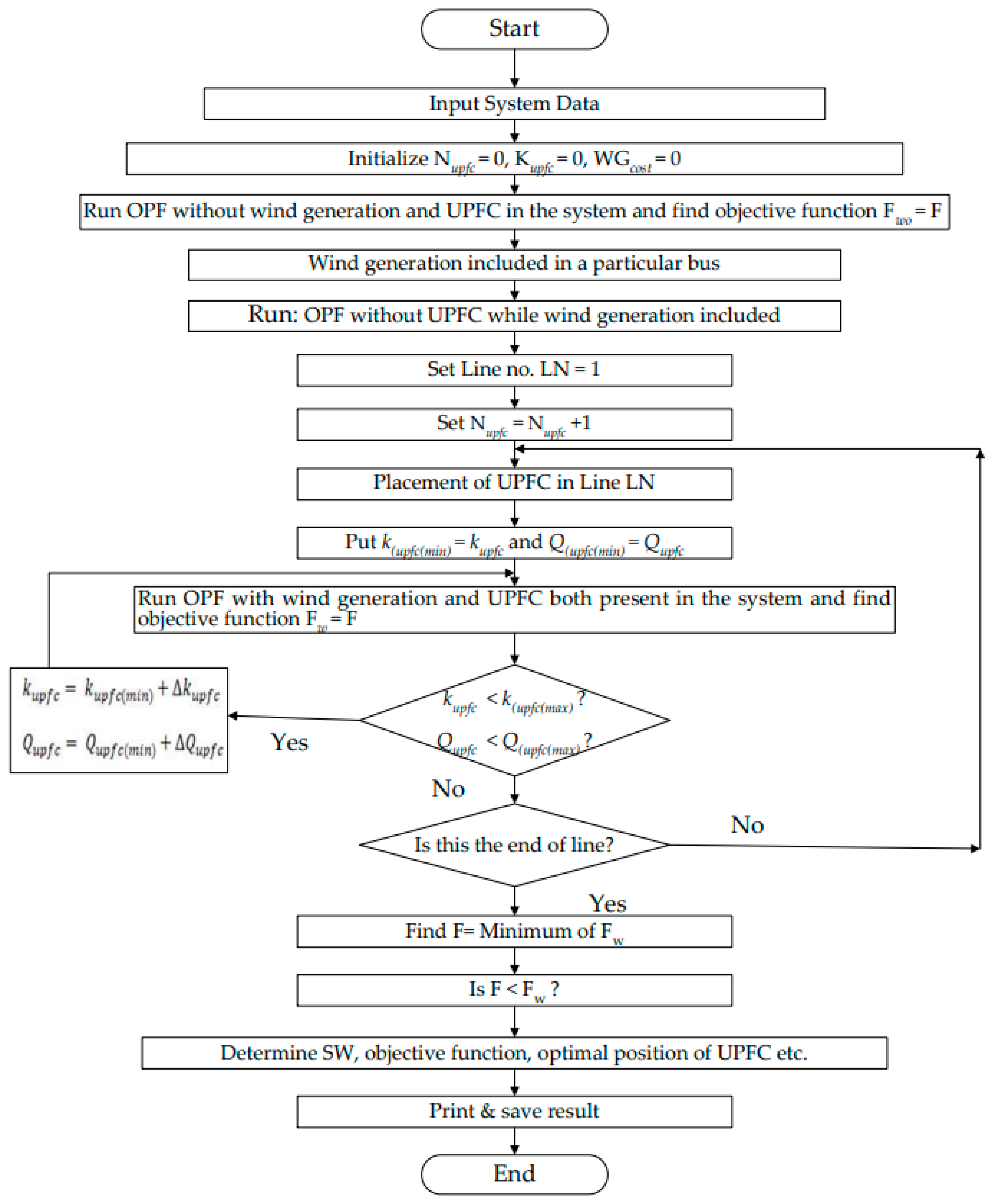
This paper outlines a method to choose the best UPFC location and cost to accomplish the objective function’s minimal value with all constraints (as mentioned in Equations (32)–(42)). In this method, optimization was carried out by positioning the UPFC, adjusting all control parameters within the predetermined bounds, and obtaining the best results. The UPFC will be placed at the optimal location where the objective function has the minimum value. For each prospective location of the UPFC, the optimum power flow has been repeatedly examined in this study.

3.4. Fuel Cell Constraints

Energy is stored using a hydrogen energy storage system made up of hydrogen tanks, an electrolyzer, and a fuel cell. Because electricity is less expensive during off-peak hours, energy is transformed into hydrogen by the electrolyzer and is preserved in hydrogen tanks. In the future, when energy prices are high during peak hours, a fuel cell can generate power using hydrogen that has accumulated. The following factors determine the electrolyzer’s operation [40,41]:

$${\mathrm{E}}_{\mathrm{elz}\left(\min \right)} \le { \mathrm{E}}_{\mathrm{elz}}\le {\mathrm{E}}_{\mathrm{elz}\left(\max \right)}$$

(43)

$${\mathrm{E}}_{{\mathrm{H}}_{2\left(\min \right)}}^{\mathrm{p}} \le { \mathrm{E}}_{{\mathrm{H}}_2}^{\mathrm{p}}\le {\mathrm{E}}_{{\mathrm{H}}_{2\left(\max \right)}}^{\mathrm{p}}$$

(44)

The following factors determine the fuel cell’s operation:

$${\mathrm{E}}_{\mathrm{fc}\left(\min \right)} \le { \mathrm{E}}_{\mathrm{fc}}\le {\mathrm{E}}_{\mathrm{fc}\left(\max \right)}$$

(45)

$${\mathrm{fc}}_{{\mathrm{H}}_2\left(\min \right)}^{\mathrm{con}} \le { \mathrm{fc}}_{{\mathrm{H}}_2}^{\mathrm{con}}\le {\mathrm{fc}}_{{\mathrm{H}}_2\left(\max \right)}^{\mathrm{con}}$$

(46)

4. Proposed Approach

This research illustrates an optimization strategy for allocating UPFC devices in the wind power-integrated deregulated electricity system. This paper suggests a way for assessing system risk and social benefit in a wind–fuel cell-incorporated deregulated power system. For 24 h situations, the technique takes into account the implications of a disagreement between the anticipated and actual wind speeds.

Proposed Approach	Expectation
Fuel cell + Wind power	Improvement in imbalance cost and social welfare
Optimal placement of UPFC	Improvement in system risk mitigation, line flow, and enhanced voltage stability
Fuel cell + Wind power + Optimal placement of UPFC	Improvement in social welfare, system risk, voltage stability, and line flow

4.1. Algorithm for Placing UPFC

This approach finds the objective function for each situation by placing a UPFC in each line of the system, separately. In the end, UPFCs are placed along the lines with the least objective function values. A flowchart showing the said approach is shown in Figure 3, where ‘${\mathrm{N}}_{\mathrm{upfc}}$’ indicates the number of UPFCs, ‘WGcost’ indicates the cost of wind generation, and ‘Δ${\mathrm{k}}_{\mathrm{upfc}}$’ indicates the increment in ‘${\mathrm{k}}_{\mathrm{upfc}}$’.

4.2. Application of the Proposed Approach

This work has been conducted using a modified IEEE 30-bus system to evaluate the efficacy of the suggested technique. MATPOWER was used in this study to find the solution to the optimal power flow problem. Flowcharts of profit calculation and risk assessment are shown in Figure 4 and Figure 5.

4.3. Integration of a UPFC and a WPG on a Modified IEEE 30-Bus System

In this research, a modified IEEE 30-bus system is utilized to examine how the recommended approach works. The test system’s information is gathered from [42,43]. The OPF problem was initially solved using SQP, and several meta-heuristic optimization techniques were subsequently applied for comparison studies.

5. Results and Analysis

Three system scenarios were evaluated to substantiate the suggested technique and demonstrate the effects of a WPG and a UPFC in the system:

(a)

Regulated system;

(b)

Deregulated system with single-demand bus auction bidding;

(c)

Deregulated system with double-demand bus auction bidding.

In addition, the system was analyzed considering the following cases:

• System performance in the absence of a WPG and a UPFC;
• System performance when only a WPG is present;
• System performance when a WPG is present and the UPFC is optimally located.

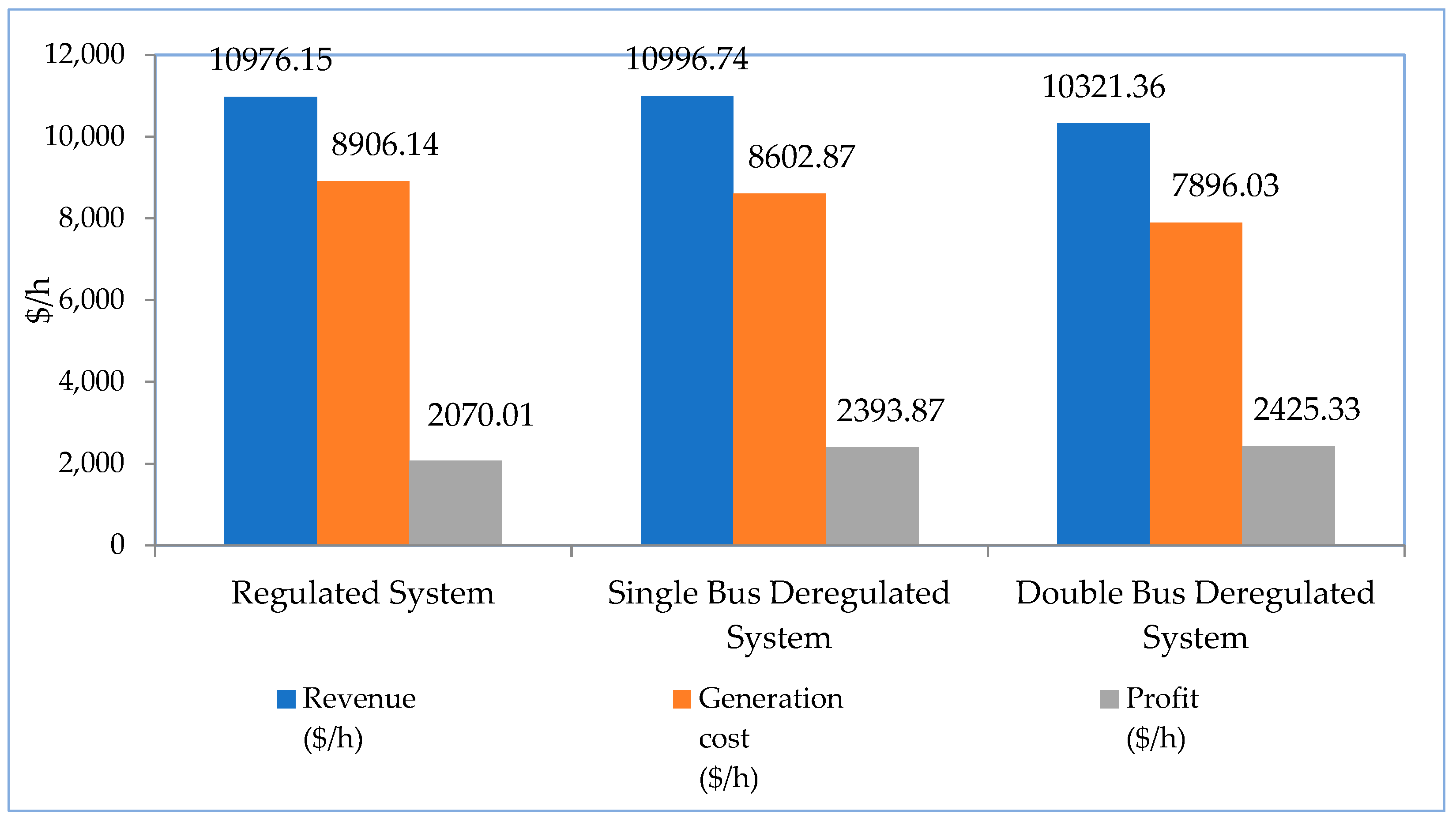
5.1. Case 1: Performance of the System in the Absence of a WPG

The OPF in a modified IEEE 30-bus system in the absence of a wind generator has been performed. The generating cost, system revenue, and profit for various systems are displayed in Figure 6. The data for all generators for the various cases under consideration are provided in

Table 3. Comparison of generation data of various systems.

Wind Speed (m/s)	Generator 1			Generator 2			Generator 3			Generator 4			Generator 5
	Regulated System	Single-Bus Deregulated System	Double-Bus Deregulated System	Regulated System	Single-Bus Deregulated System	Double-Bus Deregulated System	Regulated System	Single-bus Deregulated System	Double-Bus Deregulated System	Regulated System	Single-Bus Dgulated System	Double-Bus Deregulated System	Regulated System	Single-Bus Deregulated System	Double-Bus Deregulated System
1.67	212.16	212.18	210.78	36.22	36.22	35.98	28.99	29	25.65	12.67	12.66	6.24	4.09	4.05	0
1.94	212.12	212.14	210.73	36.21	36.21	35.97	28.74	28.78	25.41	12.48	12.5	6.04	3.88	3.87	0
2.22	212.07	212.08	210.66	36.2	36.2	35.96	28.49	28.5	25.11	12.29	12.29	5.78	3.66	3.63	0
2.50	212	212.01	210.58	36.19	36.19	35.95	28.12	28.14	24.71	12.02	12.02	5.45	3.35	3.31	0
2.78	211.91	211.93	210.48	36.17	36.17	35.93	27.67	27.68	24.22	11.68	11.68	5.04	2.96	2.93	0
3.06	211.81	211.82	210.36	36.15	36.15	35.91	27.11	27.13	23.62	11.26	11.26	4.53	2.49	2.45	0
3.33	211.68	211.7	210.21	36.13	36.13	35.88	26.44	26.46	22.9	10.76	10.76	3.93	1.93	1.88	0
3.61	211.53	211.55	210.03	36.1	36.1	35.85	25.64	25.67	22.05	10.15	10.17	3.21	1.3	1.22	0
3.89	211.33	211.36	209.82	36.07	36.07	35.81	24.68	24.72	21.06	9.38	9.43	2.38	0.67	0.54	0
4.17	211.07	211.1	209.58	36.02	36.02	35.77	23.49	23.53	19.91	8.35	8.38	1.43	0.21	0.11	0
4.44	210.74	210.75	209.28	35.96	35.96	35.72	22.05	22.05	18.55	6.98	6.95	0.5	0	0.01	0
4.72	210.33	210.34	208.85	35.89	35.89	35.64	20.34	20.34	16.78	5.31	5.29	0.05	0	0	0

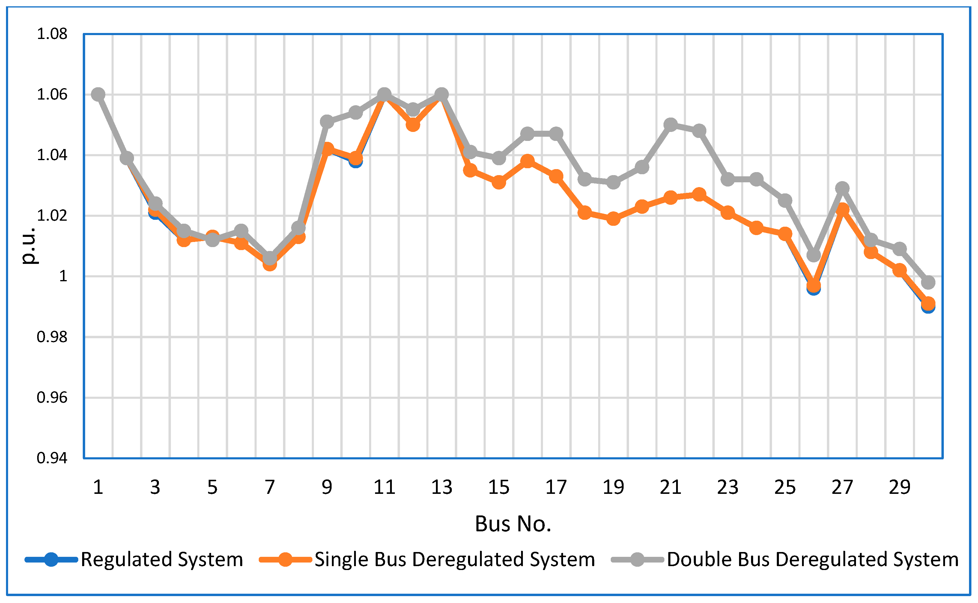
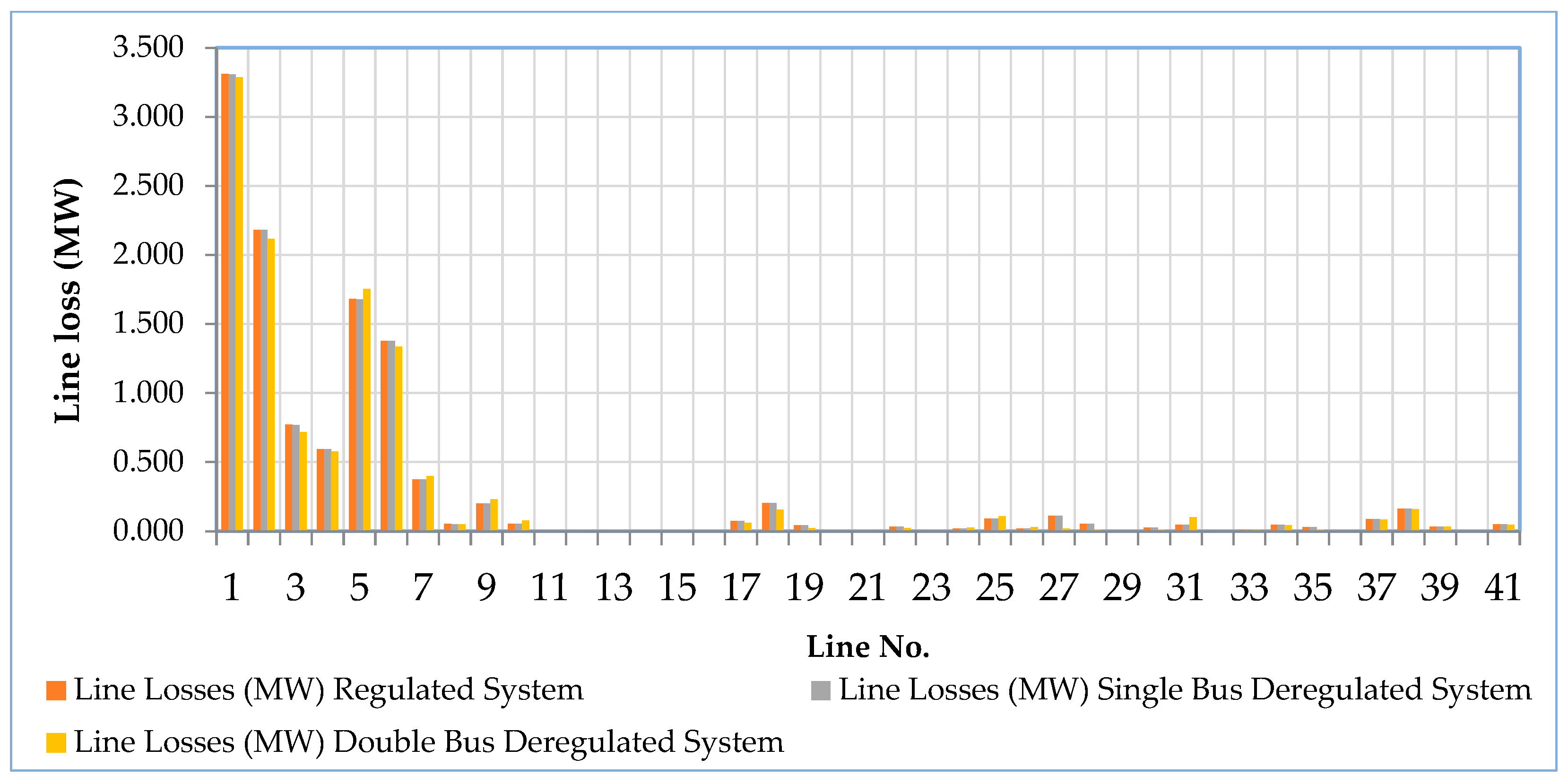
. It has been observed that demand-side bidding reduces system generating costs, directly benefiting power consumers. Demand-side bidding suggests that the present electricity system may go ahead with more deregulation. As additional buses are added to the demand-side bidding (DSB), the generating costs decrease and LMP increases, as can be seen from the results displayed in Figure 7. Various scenarios’ voltage and transmission line losses are shown in Figure 8 and Figure 9. Both tables exhibit higher improvements after the double-demand-side bidding.

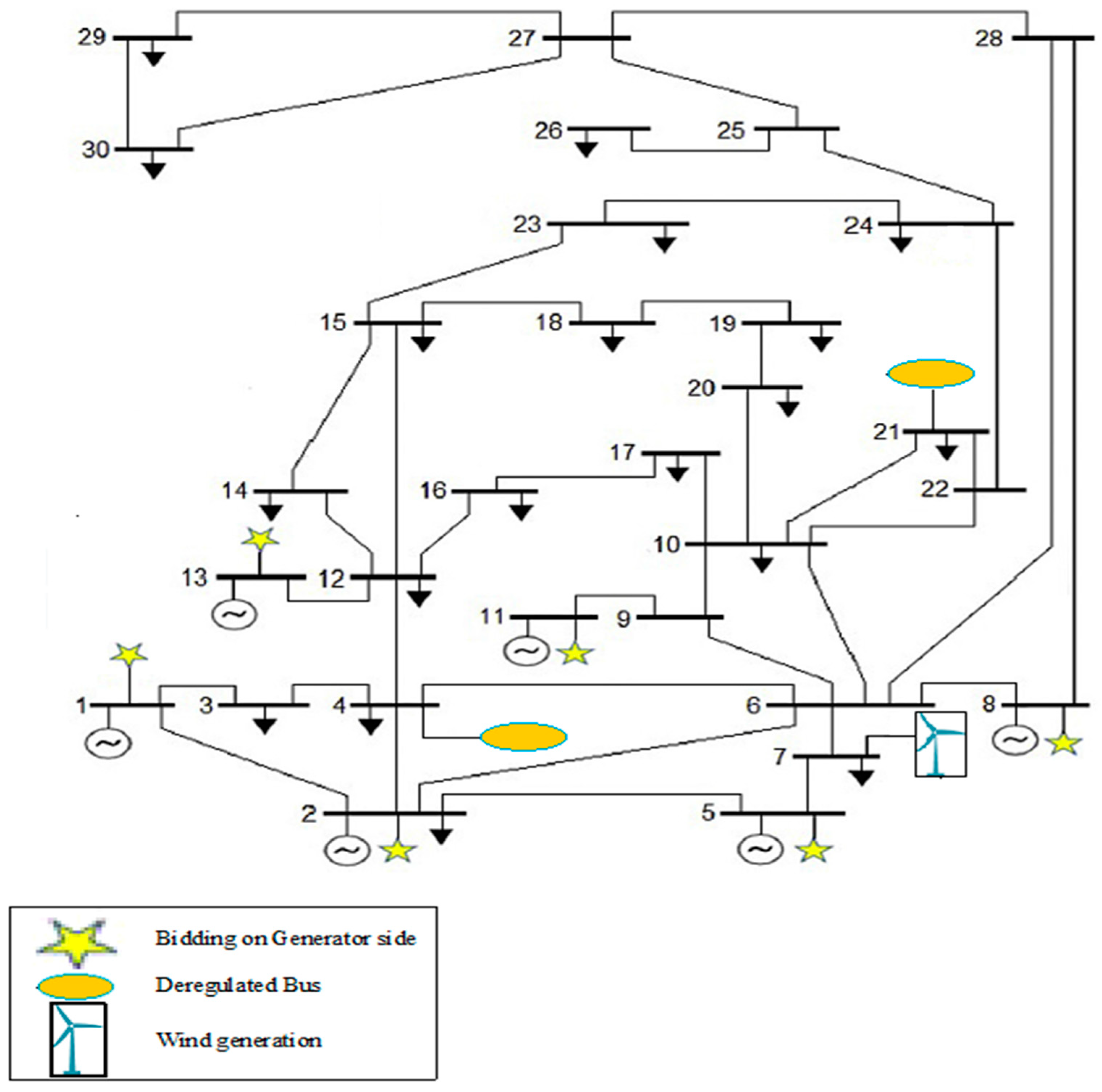
Demand-side bidding (DSB) is used for the modified IEEE 30-bus system at bus number 4 for a single-bus bidding and at bus numbers 4 and 21 for a double-bus bidding. To allow the load and generation sides some flexibility, this analysis has taken into account both generation- and demand-side biddings. Figure 10 depicts the single-line diagram for a modified IEEE 30-bus system with the bidding structure.

Demand-side and generator-side bidding have both proven effective in the deregulated power scenario. As a result, compared to the regulated system, the power scheduling procedure is altered. Customers usually become financial gainers because the electrical sector is hugely competitive. The system currently includes many generation companies, which has increased the competition and quality of the power. For these reasons, after the system is changed to a deregulated system, significant positive changes in the system voltage profile as well as in transmission line losses are observed.

From Figure 8, it is seen that the system voltage profile reaches very near to the desired 1 p.u. after the implementation of the deregulated environment compared to the regulated one. The graph indicates a more stable system condition with the deregulated environment. Table 3 shows the optimal generation capacity of each generator considering all three chosen cases. It can be seen that the generation from Generator 6 is zero for all conditions. So, it has not been included in Table 3.

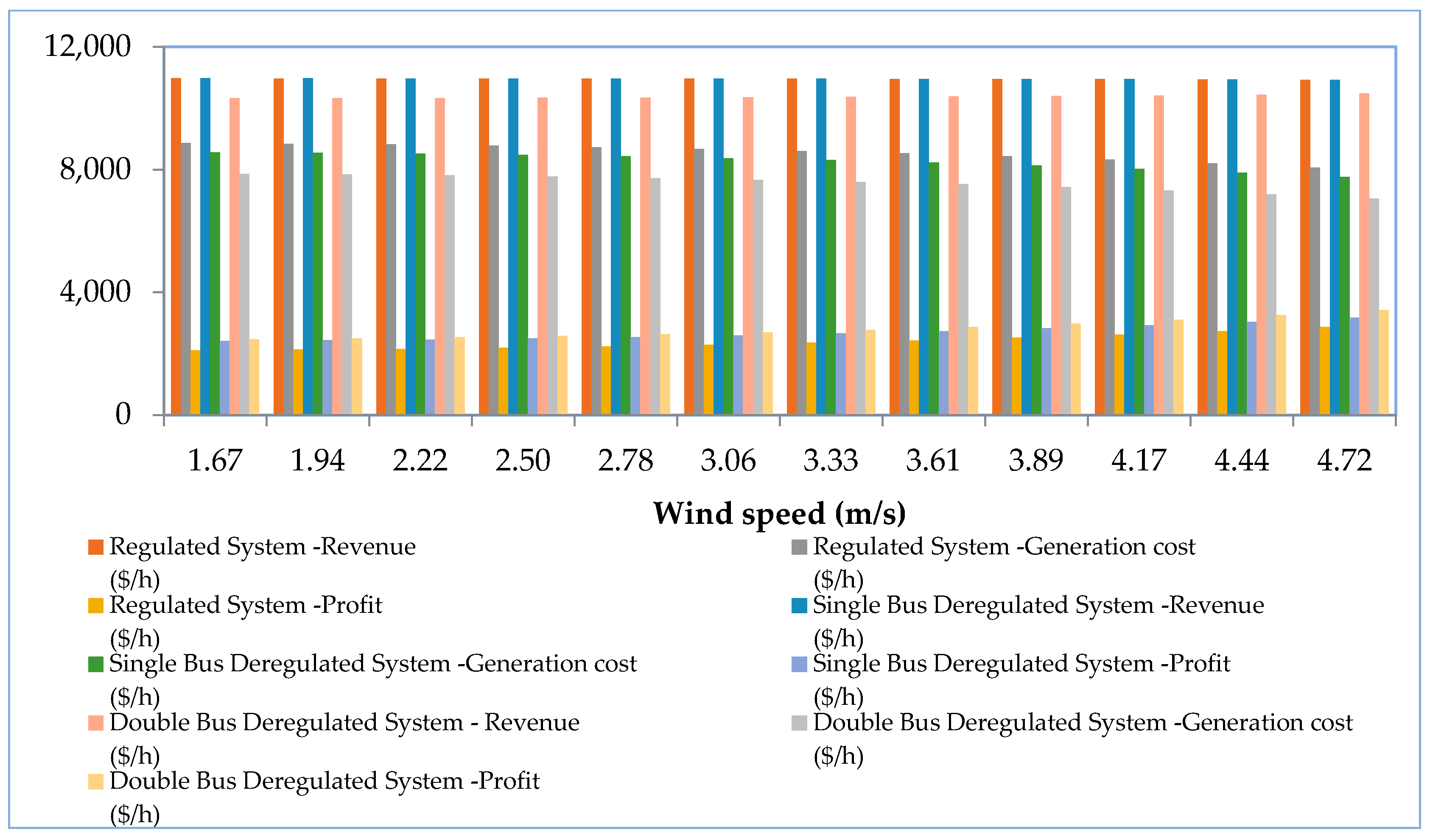
5.2. Case 2: System Performance with a WPG but without Considering the Imbalance Cost

SQP has been employed to estimate the optimum power flow, and bus number 4 has been chosen at random as the location for the wind generator. When computing the entire generating cost, which also includes the cost of generation of the thermal system, the wind investment cost is taken into account. For numerous systems with varied specified wind speeds, Figure 11 displays the revenue costs and overall generating costs. The system may experience a drop in the overall generation cost and a rise in profit as deregulation approaches.

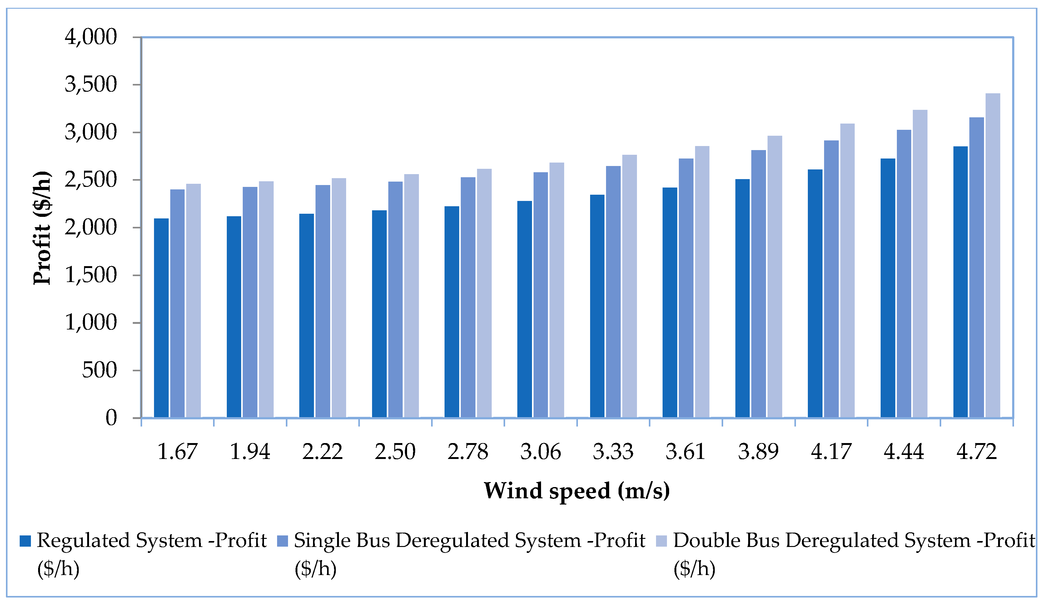
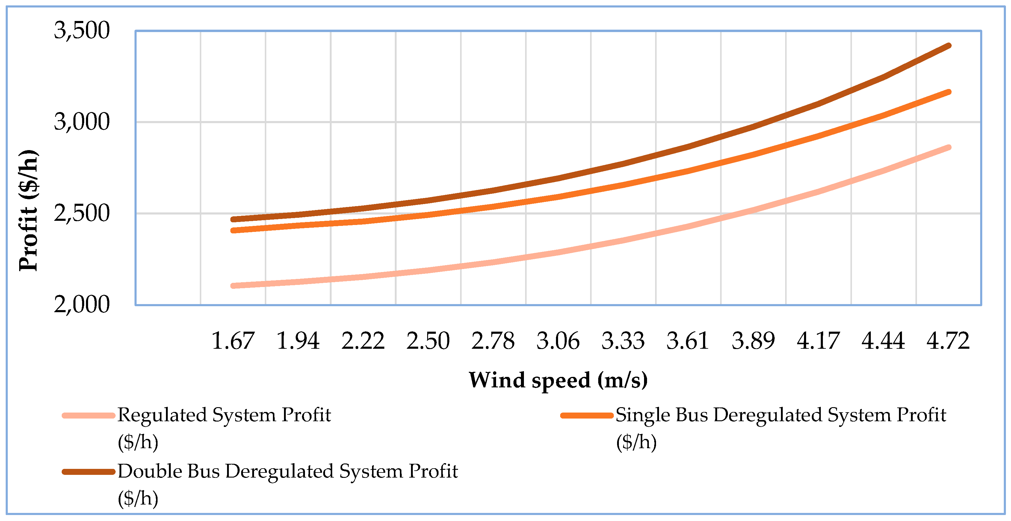
Figure 12 displays a comparison of system profits at various wind speeds. Adding more wind power into the system results in a better profit. Social welfare and system generation costs are inversely related. It is evident in this instance that adding wind farms to the system reduces generation costs, maximizing societal benefits.

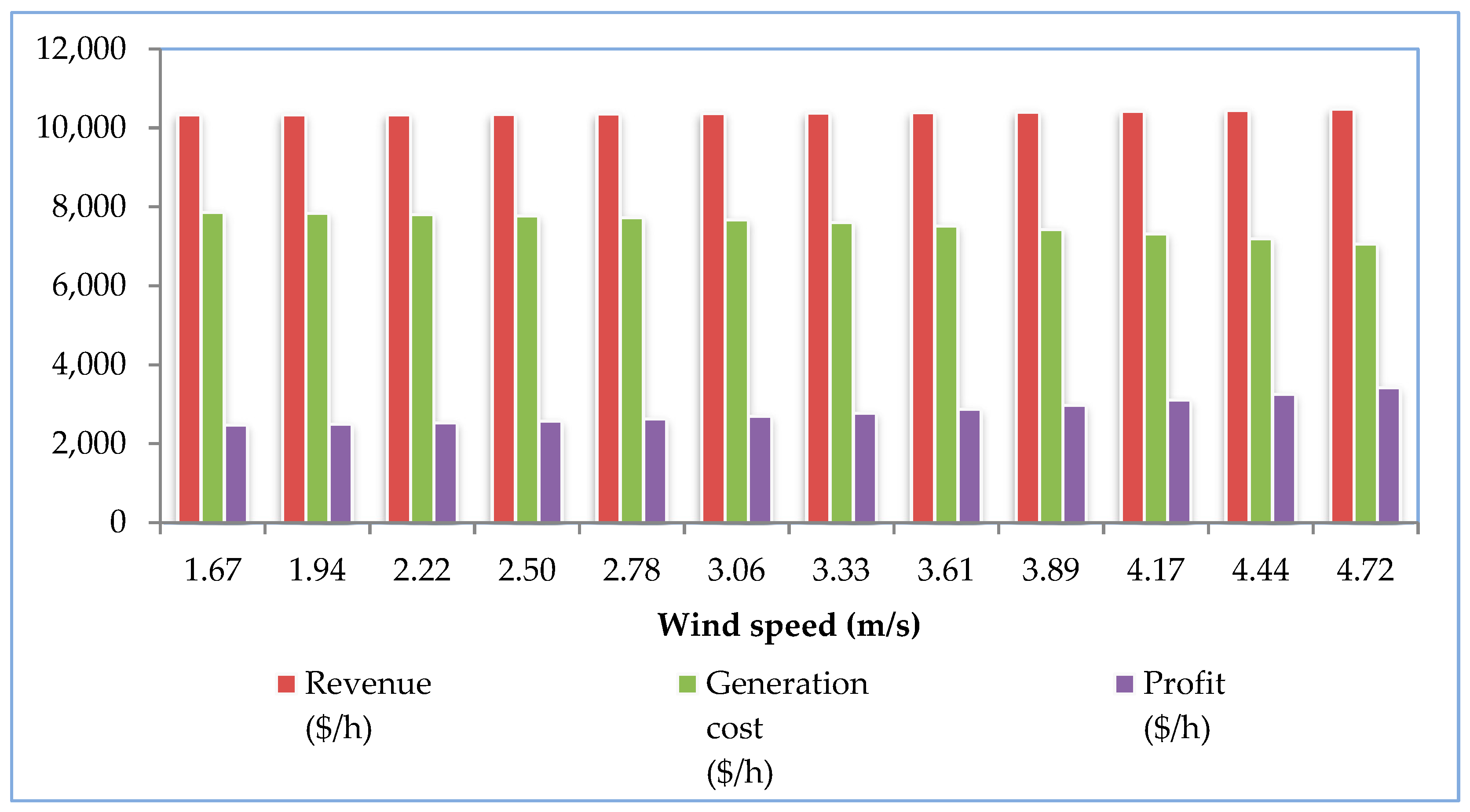
5.3. Case 3: System Performance with a WPG and Considering the Imbalance Cost

With a wind-integrated electrical system, the idea of the imbalance cost accounts for the implications of variable wind speeds on profit. The location of the wind generator inside the system was arbitrary. The wind generator in this instance was located on bus number 7, and OPF was performed for each wind datapoint while taking into consideration all of the limitations specified in Equations (32)–(40). The cost of thermal generation is estimated along with the overall cost of generating electricity after the wind generator is placed, taking the cost of the wind power investment into account. The generation cost of the thermal system fluctuates according to the circumstance due to producing rescheduling.

Figure 13 shows that the generation cost of the thermal units decreases as wind speed/wind power rises.

Table 4. Generation and LMP calculations for the modified IEEE 30-bus system after wind placement.

Wind Speed (m/s)	Gen 1		Gen 2		Gen 3		Gen 4		Gen 5		Gen 6
	Generation ($)	LMP ($/MWh)	Generation ($)	LMP ($/MWh)	Generation ($)	LMP ($/MWh)	Generation ($)	LMP ($/MWh)	Generation ($)	LMP ($/MWh)	Generation ($)	LMP ($/MWh)
1.67	210.78	36.20	35.98	37.99	25.65	40.51	6.24	40.13	0.00	39.88	0.00	39.52
1.94	210.73	36.20	35.97	37.99	25.41	40.51	6.04	40.12	0.00	39.83	0.00	39.51
2.22	210.66	36.19	35.96	37.98	25.11	40.50	5.78	40.12	0.00	39.82	0.00	39.51
2.50	210.58	36.19	35.95	37.97	24.71	40.49	5.45	40.11	0.00	39.81	0.00	39.50
2.78	210.48	36.18	35.93	37.97	24.22	40.48	5.04	40.10	0.00	39.80	0.00	39.48
3.06	210.36	36.17	35.91	37.95	23.62	40.47	4.53	40.09	0.00	39.79	0.00	39.47
3.33	210.21	36.16	35.88	37.94	22.90	40.46	3.93	40.08	0.00	39.78	0.00	39.45
3.61	210.03	36.14	35.85	37.92	22.05	40.44	3.21	40.06	0.00	39.76	0.00	39.43
3.89	209.82	36.13	35.81	37.91	21.06	40.42	2.38	40.05	0.00	39.74	0.00	39.41
4.17	209.58	36.11	35.77	37.88	19.91	40.40	1.43	40.03	0.00	39.72	0.00	39.38
4.44	209.28	36.09	35.72	37.86	18.55	40.37	0.50	40.00	0.00	39.69	0.00	39.34
4.72	208.85	36.05	35.64	37.82	16.78	40.34	0.05	39.95	0.00	39.64	0.00	39.29

indicates that LMP improves with the increase in wind speed. In all circumstances, this lowers the thermal power generation cost while enhancing wind power.

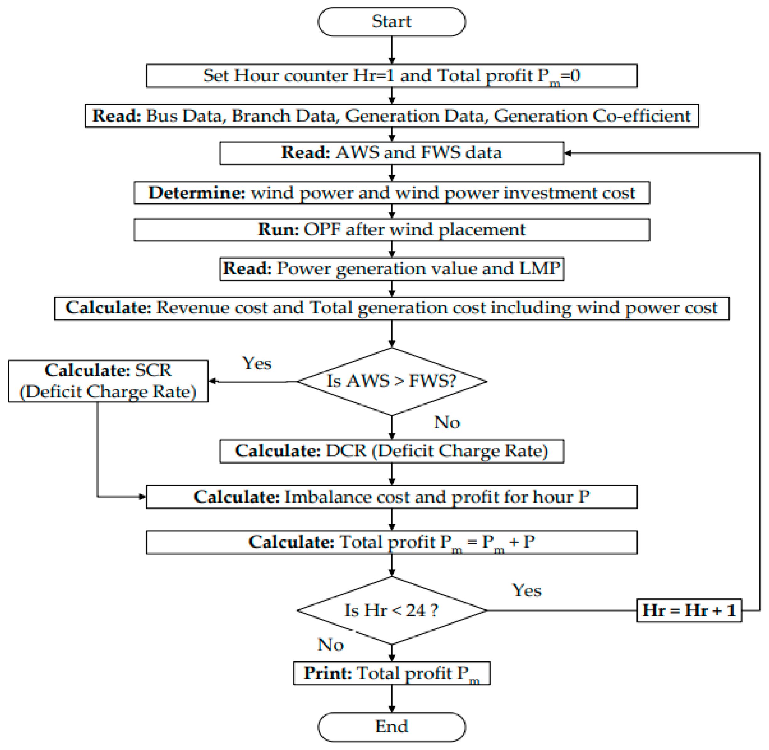
The mismatch between real wind speed data and predictions is represented by the system’s imbalance cost. The imbalance cost (negative) is largest when the disagreement between the predicted and actual wind speeds is greatest. A deficit charge rate is attained when the actual wind speed exceeds the anticipated wind speed, while a surplus charge rate is attained when the actual wind speed is lower than the anticipated wind speed. By taking the deficit and excess charge rates into consideration, we can determine the total imbalance cost of the electrical system. If the projected and actual wind speeds match, there is no cost associated with the imbalance. There is a certain number of hours in city situations where the cost of the imbalance is zero, as shown in

Table 5. Imbalance cost (in $/h) calculations for 24 h.

Hour	Delhi	Mumbai	Hour	Delhi	Mumbai
1	0	0	13	3.0727	6.3861
2	4.189	3.0727	14	0	6.5408
3	4.189	−48.4454	15	0	6.4891
4	4.189	0	16	0	0
5	2.4329	0	17	0	−404.6408
6	2.4329	−48.4454	18	0	−671.0034
7	4.189	−48.4454	19	0	−499.7596
8	2.4329	−62.157	20	0	−285.583
9	5.2252	−77.2631	21	0	−77.2631
10	6.7857	−171.9853	22	−48.4454	−62.157
11	4.189	0	23	−48.4454	−48.4454
12	4.189	9.6045	24	0	0

. It is the outcome of the precise wind speed forecasts. The 24 h interval system’s imbalance cost is also shown in Table 5 for each selected location in India. The “positive” imbalance cost means that GENCOs are rewarded by the ISO for supplying more power as opposed to being penalized by the ISO for providing inadequate power, which contrasts with the “negative” imbalance cost.

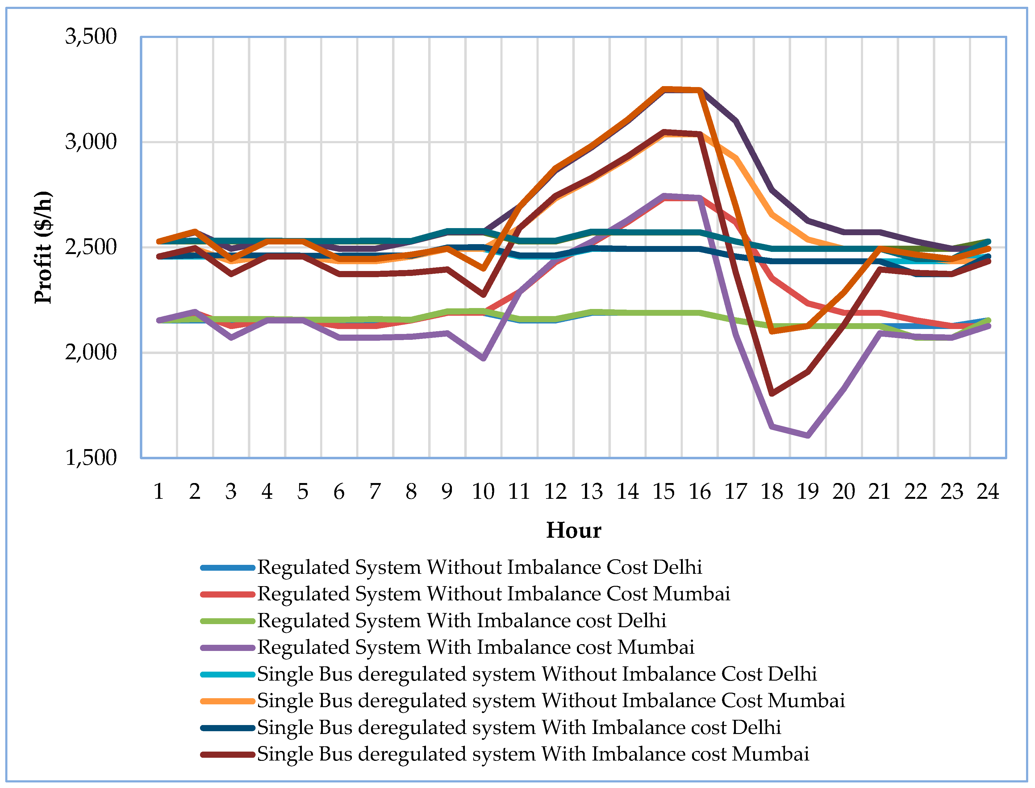
5.4. Estimated Profit throughout the Day

An electrical system’s profit at any moment is primarily determined by its revenue cost and production cost. A comparison between projected and actual wind speeds has been conducted in this study to include the imbalance cost factors in the system’s profit calculation.

Table 6. Profit (in $/h) estimation of the system for 24 h.

Hour	Delhi	Mumbai	Hour	Delhi	Mumbai
1	2527.760	2527.760	13	2574.730	2981.502
2	2531.949	2574.730	14	2571.657	3107.078
3	2531.949	2445.352	15	2571.657	3252.557
4	2531.949	2527.760	16	2571.657	3246.068
5	2530.192	2527.760	17	2527.760	2695.897
6	2530.192	2445.352	18	2493.797	2101.325
7	2531.949	2445.352	19	2493.797	2126.559
8	2530.192	2465.603	20	2493.797	2286.074
9	2576.883	2494.394	21	2493.797	2494.394
10	2578.443	2399.672	22	2445.352	2465.603
11	2531.949	2692.884	23	2445.352	2445.352
12	2531.949	2875.584	24	2527.760	2493.797

displays the profit values for 24 h for each site when the system is operating in a deregulated electricity environment. By lessening the negative effects of imbalance costs, the profit is raised. After the WF was installed in the system and the predicted and actual wind speed data were analyzed, Mumbai was found to have the highest profit due to more accurate forecasts of wind speed, whereas Delhi recorded the lowest profit since forecasting was less accurate.

5.5. Profit Comparison following WF Installation, Taking AWS and FWS into Account

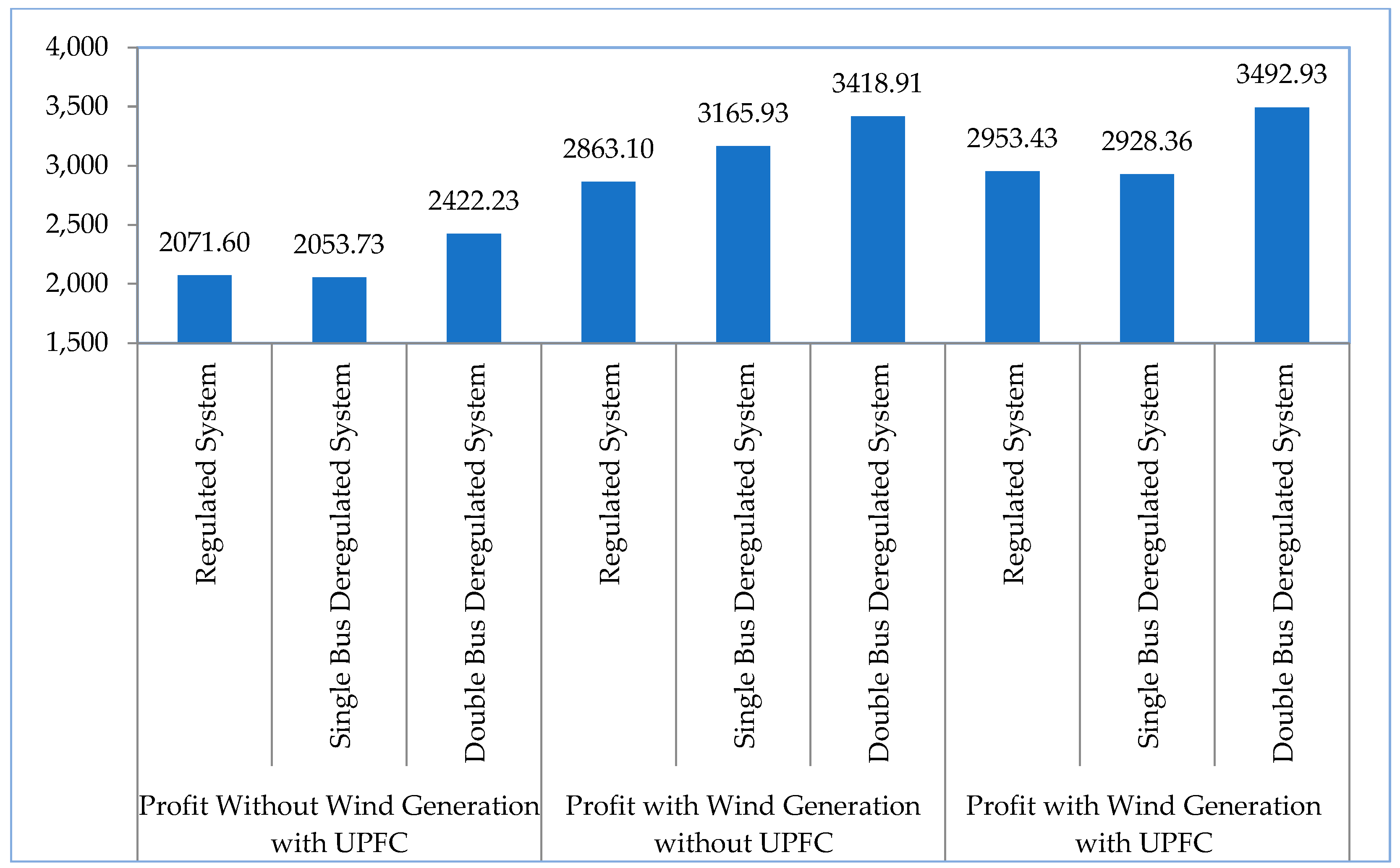
This case provides an overview of the general conclusions and findings drawn as an outcome of the deliberate work. Figure 14 shows a profit comparison while accounting for numerous scenarios for all the selected sites. It is clear that, following wind placement, profit is enhanced (Figure 15) for every site, but due to the presence of imbalance costs, profit is lowered for every location. Since wind flow is unpredictable, contracts between market participants in a deregulated power market must take this into account. When employing wind power, the system is more secure and adaptable thanks to wind speed predictions. In the event of AWS and FWS mismatch, profit can be reduced. This is supported by the data in

Table 7. Comparison of hourly profit ($/h) of Mumbai considering imbalance costs.

Hour	Regulated System	Single Bus Deregulated System	Double Bus Deregulated System	Hour	Regulated System	Single Bus Deregulated System	Double Bus Deregulated System
1	2153.898	2457.195	2527.760	13	2526.688	2829.709	2981.502
2	2193.581	2496.683	2574.730	14	2629.028	2932.696	3107.078
3	2071.723	2373.628	2445.352	15	2744.802	3048.138	3252.557
4	2153.898	2457.195	2527.760	16	2734.410	3037.441	3246.068
5	2153.898	2457.195	2527.760	17	2085.540	2380.981	2695.897
6	2071.723	2373.628	2445.352	18	1649.467	1805.740	2101.325
7	2071.723	2373.628	2445.352	19	1606.301	1909.194	2126.559
8	2075.577	2378.883	2465.603	20	1829.428	2132.467	2286.074
9	2091.728	2395.522	2494.394	21	2091.728	2395.522	2494.394
10	1972.335	2275.447	2399.672	22	2075.577	2378.883	2465.603
11	2288.263	2591.590	2692.884	23	2071.723	2373.628	2445.352
12	2441.456	2744.366	2875.584	24	2126.452	2434.508	2493.797

and

Table 8. Comparison of hourly profit ($/h) of Delhi considering imbalance costs.

Hour	Regulated System	Single Bus Deregulated System	Double Bus Deregulated System	Hour	Regulated System	Single Bus Deregulated System	Double Bus Deregulated System
1	2153.898	2457.195	2527.760	13	2193.581	2496.683	2574.730
2	2159.079	2462.349	2531.949	14	2189.747	2492.862	2571.657
3	2159.079	2462.349	2531.949	15	2189.747	2492.862	2571.657
4	2159.079	2462.349	2531.949	16	2189.747	2492.862	2571.657
5	2156.641	2460.228	2530.192	17	2153.898	2457.195	2527.760
6	2156.641	2460.228	2530.192	18	2126.452	2434.508	2493.797
7	2159.079	2462.349	2531.949	19	2126.452	2434.508	2493.797
8	2156.641	2460.228	2530.192	20	2126.452	2434.508	2493.797
9	2195.966	2499.319	2576.883	21	2126.452	2434.508	2493.797
10	2198.105	2501.179	2578.443	22	2071.723	2373.628	2445.352
11	2159.079	2462.349	2531.949	23	2071.723	2373.628	2445.352
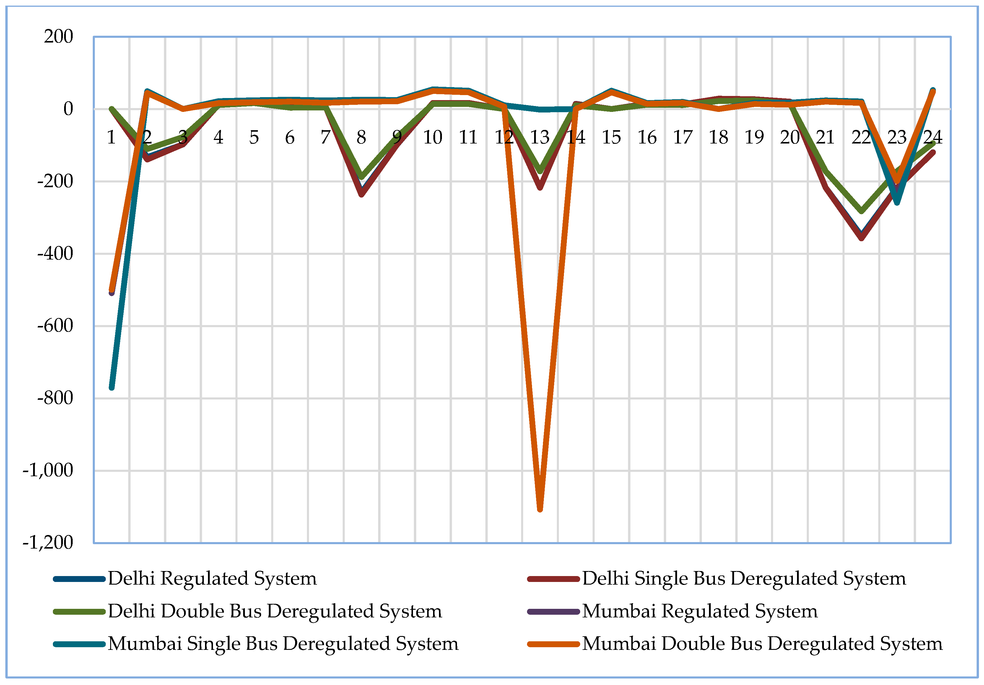
12	2159.079	2462.349	2531.949	24	2153.898	2457.195	2527.760

. A summary of the variations in the imbalance costs for the various instances taken into consideration for 24 h is shown in Figure 16.

5.6. Case 4: Performance of System with a UPFC and Wind Farm Installation

Using this test system, six generators, thirty buses, forty-one transmission lines, and nineteen loads were employed to assess the efficacy of the suggested strategy. The system information is available in [43]. Here, three test system situations were looked at to validate the methodology that was described and to demonstrate the effects of WPGs and UPFCs:

(1)

Performance of the system in the absence of a WPG and a UPFC.

(2)

Performance of a WPG-based system without a UPFC.

(3)

Performance of a WPG-based system with optimal UPFC placement.

First, OPF was performed without a WPG or a UPFC, and the total generating cost was calculated to be 550.067 $/h. The 23.04 MW wind generator is connected to bus number 7 in the system being illustrated. The hourly investment cost of a 1 MW wind power generator is $3.75 (approx.) according to [25].

In this instance, the modified IEEE 30-bus system’s OPF was obtained without WPG and UPFC placement, and the resulting total generation cost was determined to be $550.0674 per hour. Then, the 23.04 MW wind power generator was coupled to bus number 7 in the method. The bus number that the WPG was attached to was chosen at random. For all the cases under consideration, the analysis was conducted with and without the optimal placement of the UPFC. In our case, the UPFC has been taken into account for optimal placement in the system, and the relevant data are shown in

Table 9. UPFC optimal location data for different cases.

	Regulated without WPG	Regulated with WPG	Single-Bus Deregulated without WPG	Single-Bus Deregulated with WPG	Double-Bus Deregulated without WPG	Double-Bus Deregulated with WPG
UPFC Optimal Location at Line No.	5	5	5	5	9	5
UPFC Optimal Location at Bus No.	2	2	2	2	6	2
Optimal Value of UPFC (X_range of series side)	−0.25	−0.25	−0.25	−0.25	0.2	−0.25
Optimal Value of UPFC (X_range of shunt side)	−2	−2	−2	−2	−2	−2

. For the maximum scenarios, it is seen that the optimal values of reactance and reactive power injection through the UPFC are same. It indicates the stability of the system with respect to the economy. In this study, the UPFC compensation coefficient was chosen to be between (−0.7) and 0.2, while the range for reactive power injection or extraction was estimated to be between (−100) and 100. These two controlling variables change at regular intervals, and OPF was performed in every case to determine the best outcome. The total system profit has been seen to improve when a wind power source is connected to a bus (shown in Figure 17). Therefore, despite a high initial investment cost, more profit was achieved once the wind power generator was installed.

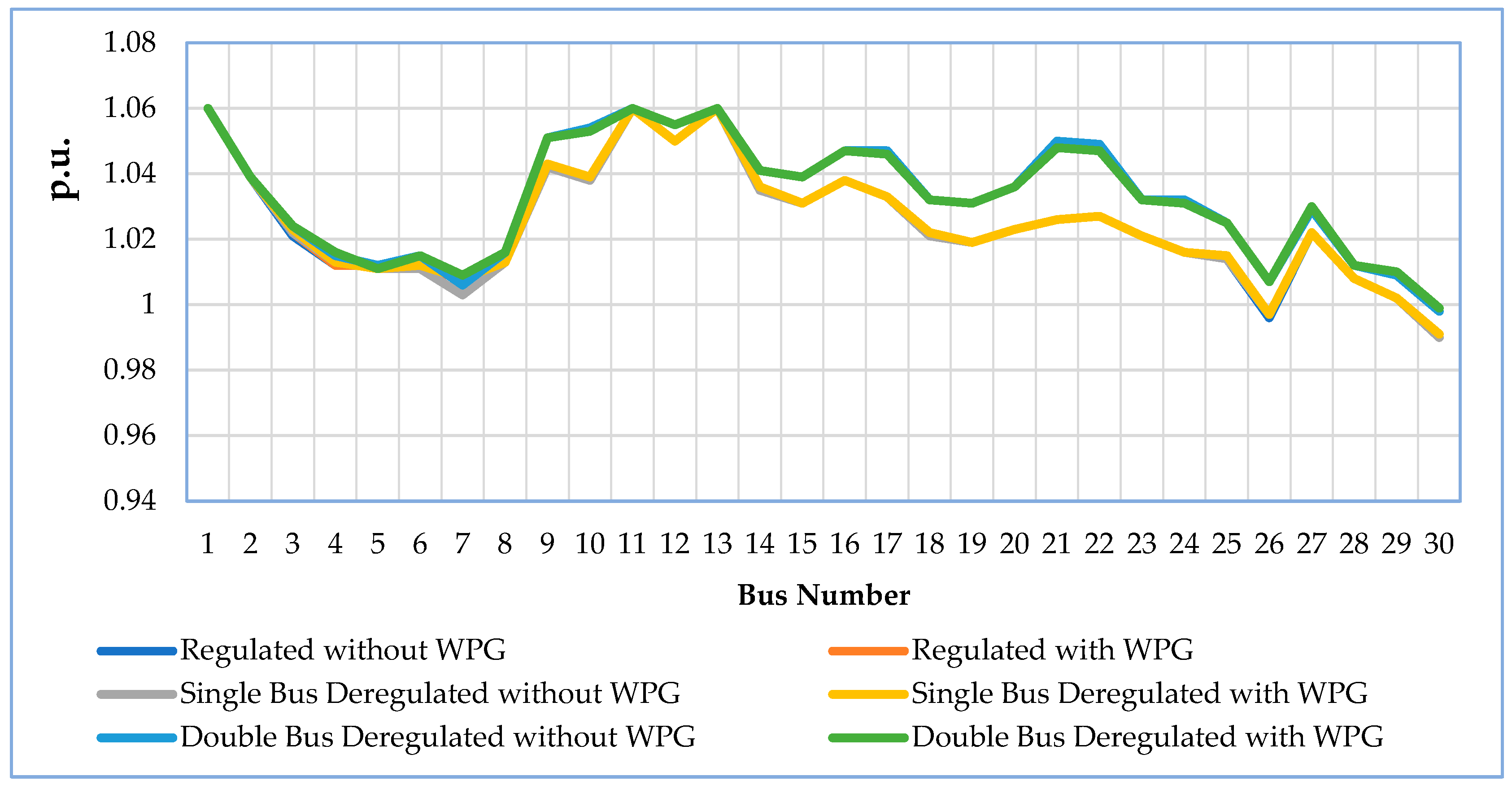
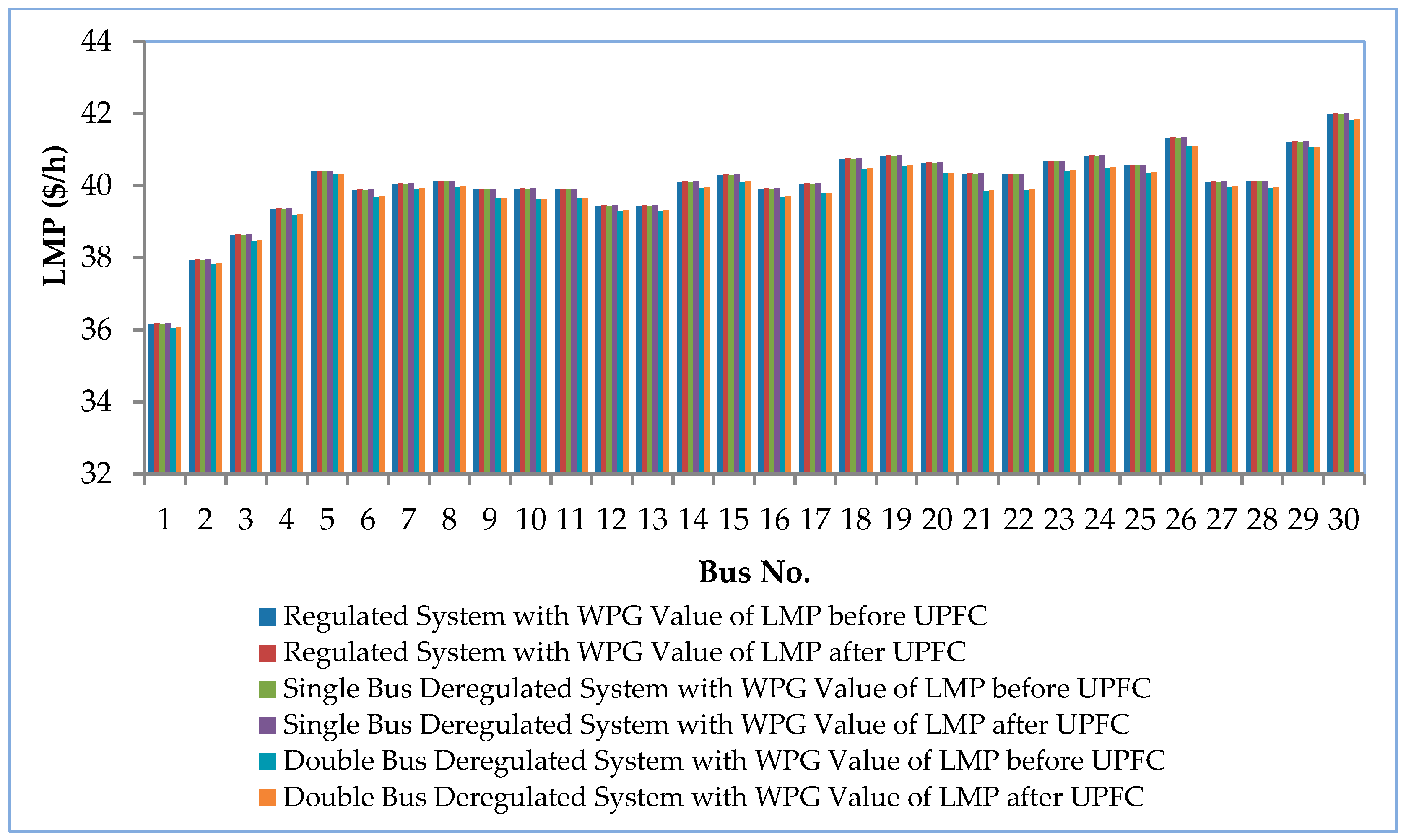
The changes in bus voltages are depicted in Figure 18. From the graphical representation of the bus voltage data as shown in Figure 18, it is clear that employing the UPFC enhanced the system’s voltage profile as well. The variation in the LMP value before and after installation of the UPFC for regulated, single-bus deregulated, and double-bus deregulated systems can be seen in Figure 19. From Figure 19, It is obvious that the LMP improved after the UPFC was installed.

5.7. Case 5: System Performance with Wind Farm and Fuel Cell Deployment

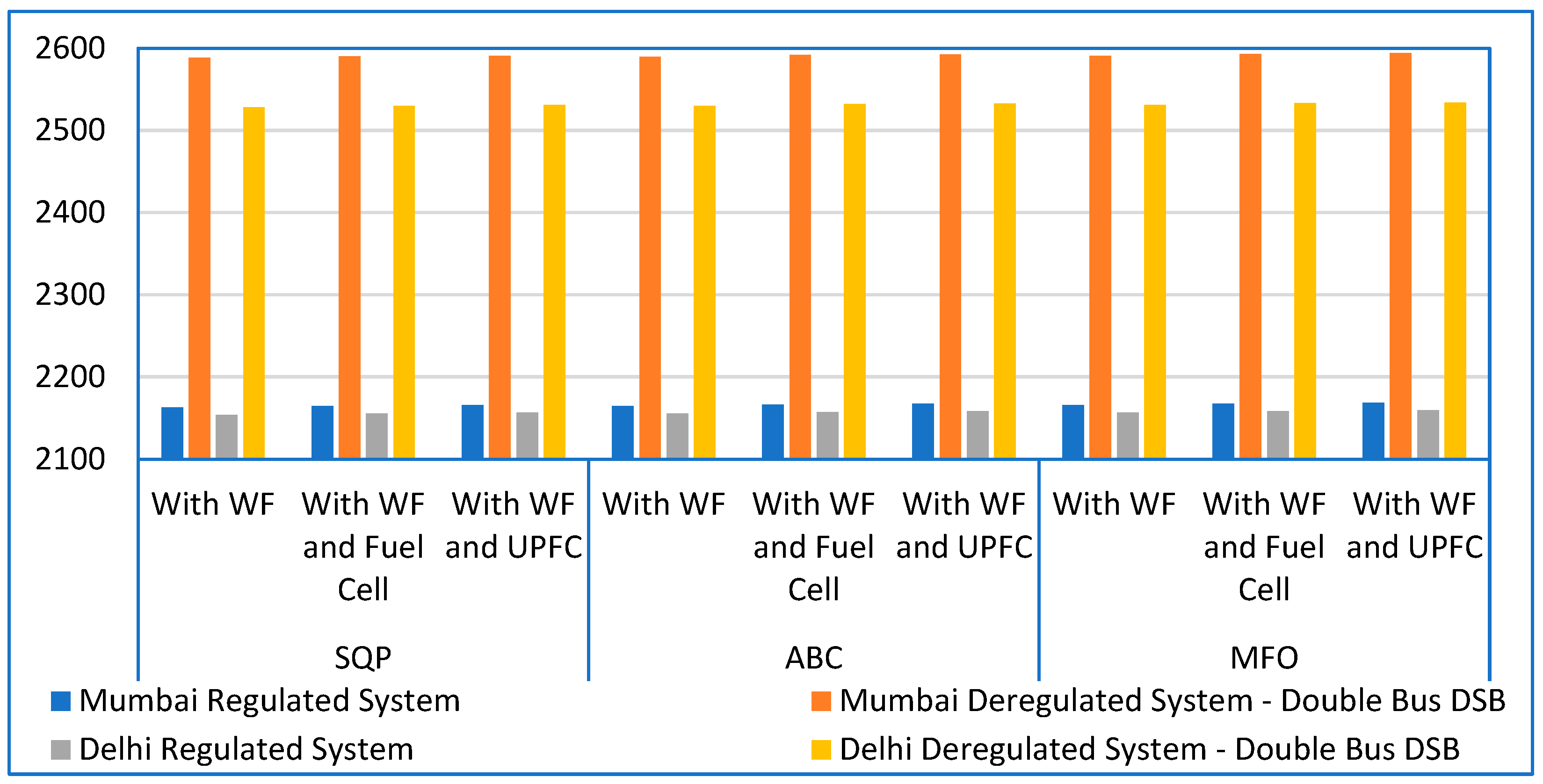
This part outlines the system economic assessments of the deregulated wind-integrated power system with the integration of fuel cells. From the preceding section, it is clear that the negative effects of imbalance costs reduce system profit. By installing the fuel cell system, the cost imbalance problem may be resolved. When wind power is available and during off-peak load periods, the fuel cell operates in charging mode. During peak load periods, it operates in discharge mode. Fuel cells can add some extra power to the system during periods of high load and lessen the difference between the planned and actual wind power schedules. In the modified IEEE 30-bus system, a fixed generating capacity with a 4 MW fuel cell system has been installed on bus number 6. The bus for the installation of the fuel cell was chosen using the logic of the greatest number of transmission lines connected to that particular bus.

Different optimization techniques, such as ABC and MFO, have been used alongside SQP to test the capabilities and applicability of the given method. The controlling variables for the MFO and ABC algorithms were taken from references [25,44,45,46,47]. The average hourly profits for Mumbai and Delhi using various optimization strategies are shown in

Table 10. Average hourly profit for Mumbai and Delhi using various optimization strategies.

Optimization Techniques	Conditions	Mumbai		Delhi
		Regulated System	Deregulated System—Double-Bus DSB	Regulated System	Deregulated System—Double-Bus DSB
SQP	With WF	2162.956	2588.267	2153.843	2528.186
	With WF and Fuel Cell	2164.625	2589.924	2155.538	2529.965
	With WF and UPFC	2165.538	2590.837	2156.429	2530.854
ABC	With WF	2164.456	2589.721	2155.364	2529.725
	With WF and Fuel Cell	2166.358	2591.629	2157.219	2531.693
	With WF and UPFC	2167.235	2592.538	2158.129	2532.535
MFO	With WF	2165.563	2590.814	2156.421	2530.816
	With WF and Fuel Cell	2167.683	2592.931	2158.563	2532.927
	With WF and UPFC	2168.529	2593.824	2159.428	2533.825

and Figure 20.

The results indicate that the system profits produced by the addition of fuel cells to the system are larger than those produced by a wind-integrated electrical system without fuel cells. This paper’s fundamental novelty is in applying MFO optimization for the first time to an economic problem of this nature. In terms of system profit maximization, MFO outperforms the other two applied optimization algorithms for all consideration circumstances. The placement of the fuel cells and the use of MFO procedures thereby enhance system profits in the context of an unbalanced cost.

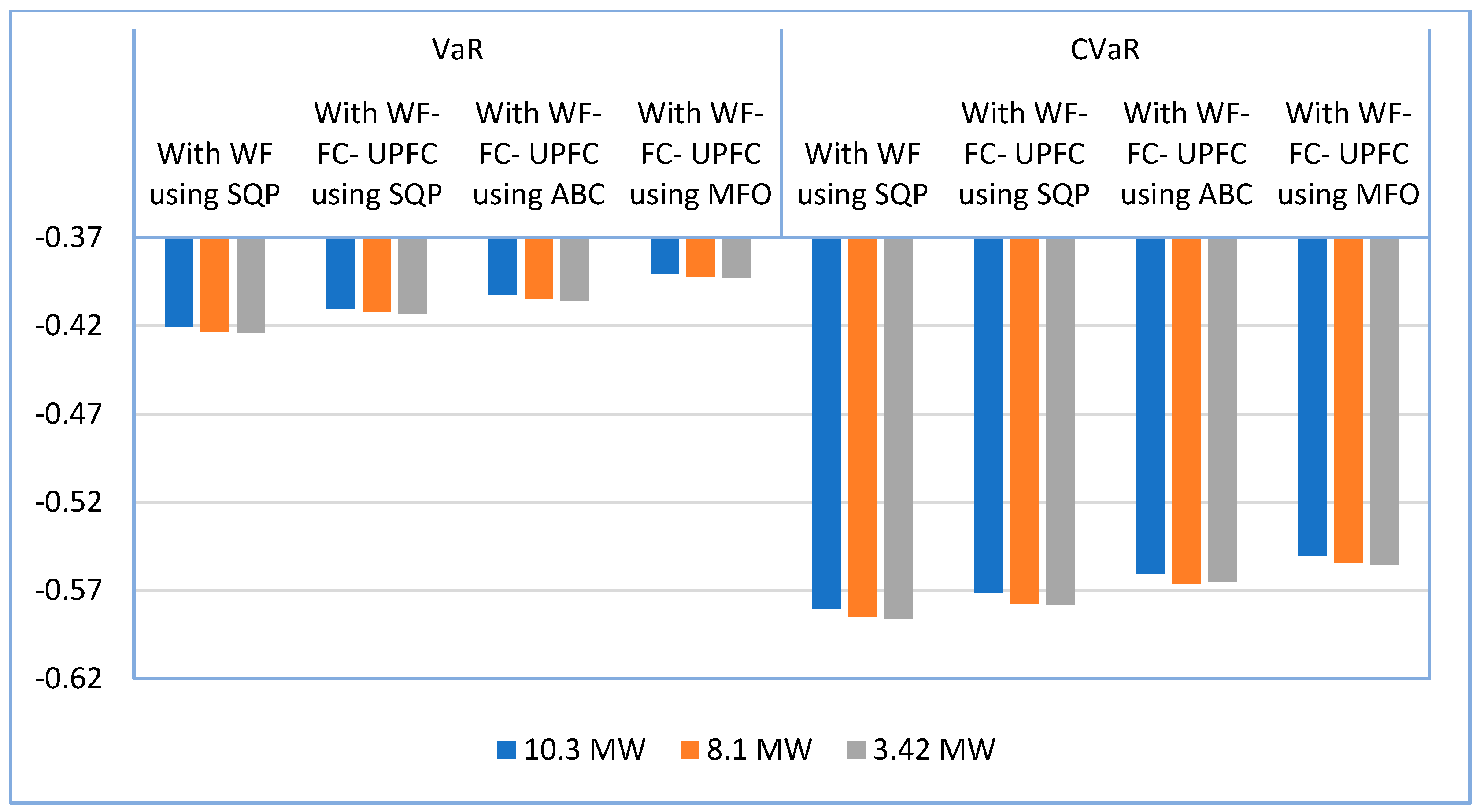
5.8. Case 6: System Risk Analysis Considering the positioning of the Wind Farm, Fuel Cell, and UPFC

The secure operation of an electrical system largely depends on system risk analysis. In the event that a fault has developed in the system, it must be fixed right away to prevent the failure of the system. The system risk has been determined using the risk analysis tools (VaR and CVaR) based on the LMP of each bus in the system under various scenarios. All of the risk data were determined with a 95% confidence level. The system risk for Delhi is shown in

Table 11. System risk for Delhi using multiple optimization techniques and various system situations.

Sl. No.	Wind Power	VaR				CVaR
		With WF Using SQP	With WF-FC-UPFC Using SQP	With WF-FC-UPFC Using ABC	With WF-FC-UPFC Using MFO	With WF Using SQP	With WF-FC-UPFC Using SQP	With WF-FC-UPFC Using ABC	With WF-FC-UPFC Using MFO
1	10.3 MW	−0.4205	−0.4103	−0.4023	−0.3907	−0.5807	−0.5714	−0.5604	−0.5504
2	8.1 MW	−0.4234	−0.4122	−0.4046	−0.3926	−0.5851	−0.5774	−0.5662	−0.5545
3	3.42 MW	−0.424	−0.4135	−0.4057	−0.393	−0.586	−0.578	−0.5653	−0.5556

and Figure 21 for various system configurations and optimization techniques. The application of MFO algorithms allows for the operation of the most wind farms with the lowest level of system risk. The system risk was decreased once the fuel cell and the UPFC were put into the system. By supplying more electricity locally, the load on the grid was reduced, which is why this occurred.

6. Conclusions

The optimum parameter settings for the UPFC and fuel cells in the regulated and deregulated power systems were presented in this research using different optimization techniques to mitigate the system risk and maximize the economic sustainability of the systems. On modified IEEE 30-bus test systems, the proposed methodology was performed. The test results demonstrated the viability of the suggested strategy. The goal of this study was to maximize societal welfare and system profit while minimizing the objective function using the cost models of UPFCs, fuel cells, and wind power generation. It has been noted that:

(a)

After adding the wind generator to the system, a UPFC was employed to mitigate the issues;

(b)

Fuel cells were successful in improving social welfare and cost imbalances;

(c)

SW became better once a UPFC was included to the pool model;

(d)

By integrating the UPFC and fuel cells with the WPG, the locational marginal price of the system significantly decreased;

(e)

The voltage profile in UPFC operation with the WPG was also stable.

This proposed approach is a universal method that may be utilized to enhance any size, type, integrated, or deregulated electrical system. In the future, this work can be performed with different renewable energy sources along with different optimization techniques to enhance system security and stability.