Article

Transformers-Based Encoder Model for Forecasting Hourly Power Output of Transparent Photovoltaic Module Systems

by
Jumaboev Sherozbek
1,
Jaewoo Park
1,
Mohammad Shaheer Akhtar
1,2,* and
O-Bong Yang
1,3,*
1
Graduate School of Integrated Energy-AI, Jeonbuk National University, Jeonju 54896, Republic of Korea
2
New and Renewable Energy Materials Development Center (NewREC), Jeonbuk National University, Buan-gun 56332, Republic of Korea
3
School of Semiconductor and Chemical Engineering, Jeonbuk National University, Jeonju 54896, Republic of Korea
*
Authors to whom correspondence should be addressed.
Energies 2023, 16(3), 1353; https://doi.org/10.3390/en16031353
Submission received: 27 December 2022 / Revised: 23 January 2023 / Accepted: 24 January 2023 / Published: 27 January 2023
(This article belongs to the Special Issue Advances in Solar Cells and Photocatalysis II)

Abstract

:
Solar power generation is usually affected by different meteorological factors, such as solar radiation, cloud cover, rainfall, and temperature. This variability has shown a negative impact on the large-scale integration of solar energy into energy supply systems. For successful integration of solar energy into the electrical grid, it is necessary to predict the accurate power generation by solar panels. In this work, solar power generation forecasting for two types of solar system (non-transparent and transparent panels) was configured by the smart artificial intelligence (AI) modelling. For deep learning models, the dataset obtained from the target value of electricity generation in kWh and other features, such as weather conditions, solar radiance, and insolation. In PV power generation values from non-transparent and transparent solar panels were collected from 1 January to 31 December 2021 with an hourly interval. To prove the efficiency of the proposed model, several deep learning approaches RNN models, such as LSTM, GRU, and transformers models, were implemented. Transformers model for forecasting power generation expressed the best model for non-transparent and transparent solar panels with lower error rates for MAE 0.05 and 0.04, and RMSE 0.24 and 0.21, respectively. The proposed model showed efficient performance and proved effective in forecasting time-series data.

1. Introduction

Maintaining a balance between efficiency and energy generation is one of the essentials for the reliable operation of solar power plants (SPP) [1]. The present solar generation facilities cannot guarantee the total electric power output at specified time. It is important that the forecast of the amount of energy generation and supply to the grid is highly relevant. Few research works have recently introduced the concept of energy meteorology (“energy-meteorology”) [2] as a new scientific discipline, the subject of which is the quantitative assessment of power generation based on renewable energy sources (RES) especially solar energy at hourly to minutes time intervals. In particular, several attentions have been paid to the hourly short-term forecast for solar energy generation forecasting. It is known that solar energy has a lot of advantages over other traditional energy sources, such as coal and natural gas; however, the power generation by photovoltaic arrays is highly variable [3,4]. Generally, the variability in solar power generation depends not only on solar radiation and temperature, but also on other meteorological factors, such as wind speed, hours of sunshine, humidity, cloud cover, and precipitation [5]. In addition, the Sun is an intermittent power source as it absorbs sunlight which is normally available in daytime. Such variability and intermittency of solar energy still challenge its large-scale integration into the energy system. So far, the energy from sun faces the unexpected changes by unwanted factors and negatively affecting the balance of the network, which resulting in increasing operating costs. Due to its irregular and unmanageable nature, an accurate solar power generation forecast is essential for the grid operator and companies supplying electrical energy from a photovoltaic system. Therefore, it is essential to develop an algorithm to maintain the stability of the power supply system. System stability can be achieved by creating methods to predict generated power and estimate future production. There are still several flaws and dependencies in the current PV power generation systems, such as temperature, humidity, and wind, which are typically caused by solar irradiation [6].
Solar energy generation forecasting methods are divided into four categories:
  • Meteorological methods: Indirect methods based on numerical weather forecasting and processing of satellite images allow first to predict the intensity of solar radiation, then convert it into the output power of a photovoltaic system.
  • Statistical methods: These methods use statistical approaches, such as the autoregressive moving average model (ARMA) [7], auto-regressive integrated moving average model (ARIMA) [8], and exponential smoothing (ES) [9]. These models can be used to directly predict the power output of photovoltaic arrays without the need first to predict solar radiation.
  • Machine learning methods: These approaches use machine learning algorithms, such as k-nearest neighbors, neural networks (NN) [10], support vector machine (SVR) [11], and pattern sequence-based forecasting (PSF) [12], to predict output directly the power of photovoltaic batteries. As a rule, there are two approaches to applying machine learning methods: building one forecasting model or combining several forecasting models to form an ensemble of forecasting models.
  • Hybrid methods: These methods combine models or different components from the previous three categories. Unlike ensembles that combine machine learning models, hybrid ones typically combine machine learning meteorological, and statistical models or their components. The use of machine learning methods, such as RNN [13] and SVR, and statistical methods, such as ARIMA and ES, are widespread for building models to predict solar plant capacity. However, most of these methods are based on one general prediction model for all meteorological conditions and their corresponding daily photovoltaic characteristics.
This work is focused on investigating the performance of existing modern deep learning methods for predicting solar power generation and create new methods for better forecasting results with improved performance. The time-series prediction model proposed in this study has a transformer structure. The original transformer architecture (Vanilla Transformer) [14] is an auto-encoder. The encoder receives a sequence with positional information as input. The decoder receives part of this sequence and the encoder output. However, the architecture of some transformer-based models consists only of an encoder. As a result, transformers maintain direct links to all previous temporal values, allowing information to reproduce over longer sequences. Another work related to transformer model has been studied [15] on the problem of forecasting influenza-like diseases. The author compared some results of various models working with time series. The base architecture is the same as the original transformers model. Adam was used as an optimizer in this work. For regularization, the authors added dropout and a dropout rate of 0.2 for each layer. In the other work [16], the authors applied the idea of creating a generative model for forecasting, where they applied generative adversarial neural networks. As a result, the error of a conventional transformer is about three times less than ARIMA (0.036). Herein, PV power generation forecasting for two solar panels (non-transparent and transparent) has been done by deep learning approaches in which some working AI models with time series are compared. Among various working models, the architecture original transformer shows the best AI model for both solar panels.

2. Experimental and Methods

2.1. Dataset

The original PV data was collected at New and Renewable Energy Materials Development center (NewREC) located in Buan-gun, Jeollabuk-do, Republic of Korea. In this work, the PV power generation data was extracted from two different solar modules, i.e., non-transparent and transparent modules, as shown in Figure 1 and details of modules summarized in Table 1. The period of collected PV data is from January to December 2021 on an hourly basis and contains weather-related information along with module energy generation outputs.
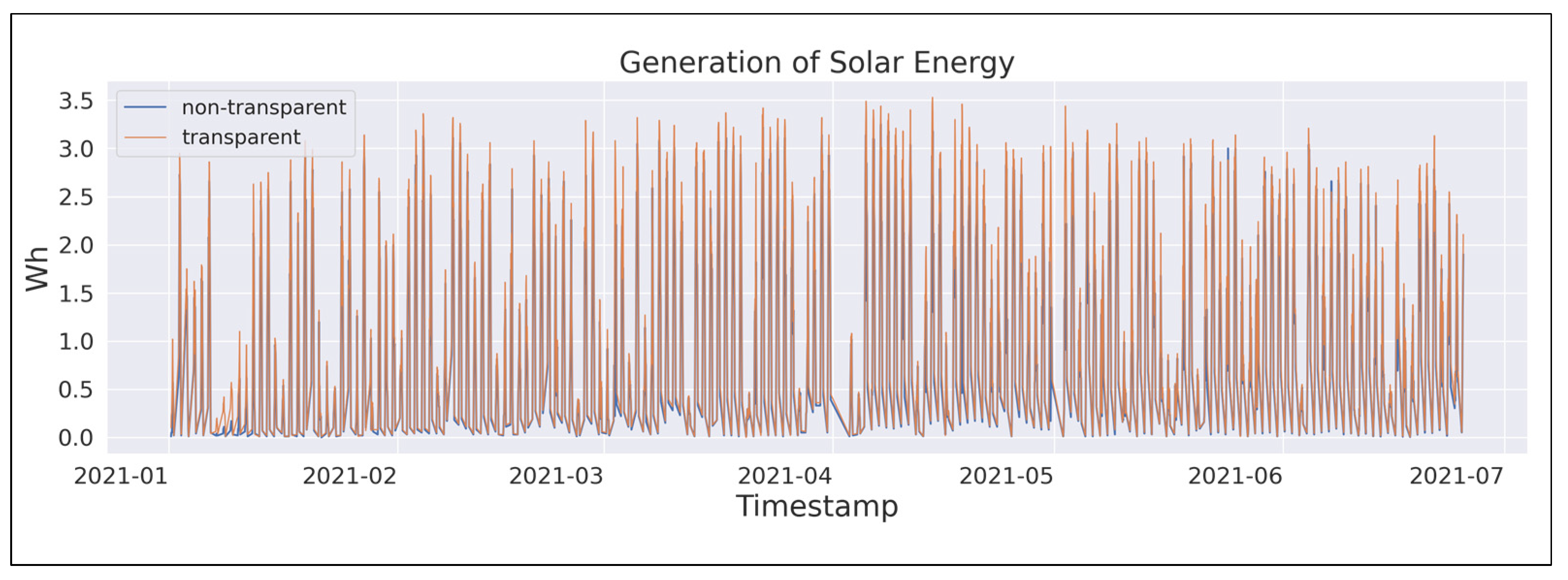
The main reason for collecting PV power generation data from two different modules in this work is to evaluate their different energy generation capability. In the case of a transparent module, the energy output is slightly higher than that of the non-transparent module due to its capability to absorb solar radiation from both sides. Bifacial transparent solar modules allow photovoltaic cells to capture reflected sunlight on the back surface. The light passes right through and collides, then bounces back towards the panels with a highly reflective surface (white roof, sandy, or rocky light soil). In our case, the surface of installed solar panels is a cement, which can reflect solar irradiation with a higher reflection rate. Table 1 shows the physical characteristics of PV modules. As seen in Figure 2, the transparent PV panels present the higher PV power generation as compared to non-transparent PV panels during the same period.
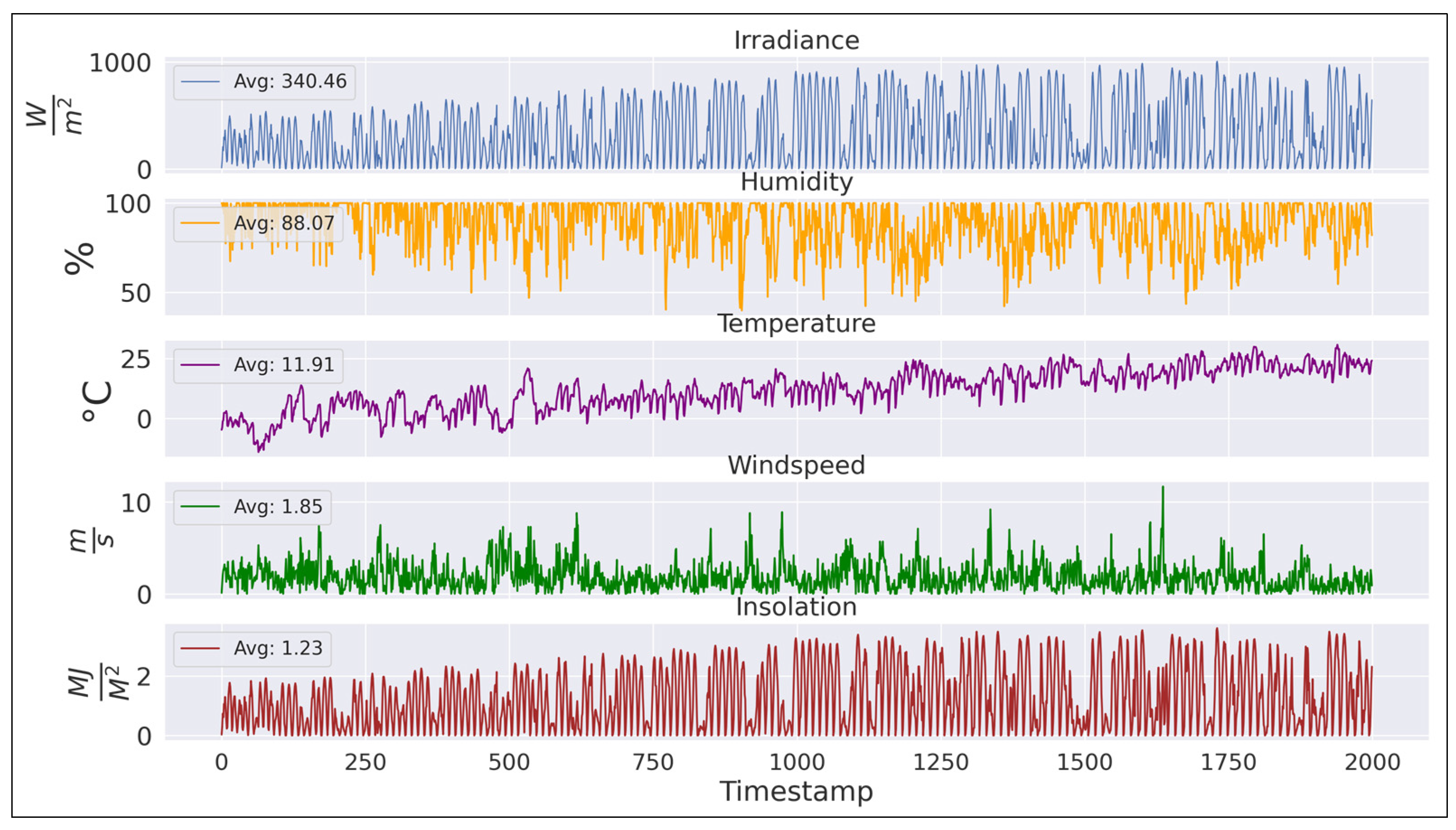
The weather data is utilized as a feature during the training process for energy forecasting, as shown in Figure 3.

2.2. Attention Based Encoder

Various computational algorithms have been developed at the academic and private sectors to increase forecasting accuracy. Transformers, a new technique in neural networks develop non-recursive modeling algorithms that specialize in predicting future elements within sequences. Transformers are initially positioned as a neural network for processing and understanding natural language [17]. One of the simplest examples is Google’s BERT language model, which is developed in 2018 [18]. However, in the four years since their inception, they have gained popularity, and have appeared in many other aspects of Deep Learning.
The traditional models, such as RNN models, are hard to train due to vanishing/exploding gradient problems, wherein older inputs have almost no effect on the output of the current stage. Additionally, the data in these models process sequentially, resulting in a poor possibility of parallelization. Even though using more powerful GPUs will not increase the speed of the training process. As a result, the processing a large amount of data is difficult. Utilizing Transformers architecture has considerable advantages over traditional RNN models. The main advantages of Transformers over LSTM [19] are reduced complexity by eliminating recurrence and parallelization technique, which improves overall computation efficiency.
In this work, the Transformers model was implemented for time-series PV power generation forecasting, and, furthermore, compared results with traditional recurrent neural network models, such as LSTM and GRU [20].
The advantage of RNN over traditional Feed-Forward Networks (FFN) is saving the input of the current layer and feeding it back in the loop form to predict the layer’s output. RNN is widely applied to solve issues of Feed-Forward Networks where FFN cannot handle sequential data. RNN also accepts not only current input, but previously received input as well. It is due to RNN’s internal memory, which memorizes historical information. However, these advantages over FFN may result in some drawbacks [21]. The Vanishing Gradient problem is the main disadvantage of using RNNs, where gradients used to compute weights become closer to zero. The deeper the model, the closer gradient to zero, resulting in a much longer computation time. The occurrence of this problem is due to certain activation functions, such as tangent hyperbolic or sigmoid functions, which squishes large input space into small output space.
To resolve these problems, a Transformer-based network is implemented, in which the recurrence is not utilized for sequential calculation. Moreover, its computation is parallelized, resulting in the acceleration of the training process. The transformer has an architecture in which several encoders are primarily accumulated. An encoder is called a Multi-Head Attention. It consists of a layer and a Feed Forward Neural Network layer. As mentioned above, the Attention module has parallelized computation repeatedly, and each repeated process is called an ‘attention head’. Primarily, the attention module has its Query, Key, and Value parameters, which are passed through the scaled dot product attention independently. Afterward, every Head is concatenated and combined with a final weight matrix. This technique is called Multi-Head Attention and is powerful for encoding multivariate time series. (Refer to [4] for more details). Figure 4A,B visualizes the implemented model with the original encoder algorithm.
The mathematical formula can be defined as:
Multihead ( Q , K , V ) = Concat ( head 1 , , head h ) W O
where h e a d i = A t t e n t i o n ( Q W i Q , K W i K , V W i V ) .
Learnable parameters of Multi-Head Attention layer:
W 1 . . h Q R D × d k , W 1 . . h K R D × d k , W 1 . . h V R D × d v     a n d       W O R h d k × d o u t
where D is the input dimensionality.
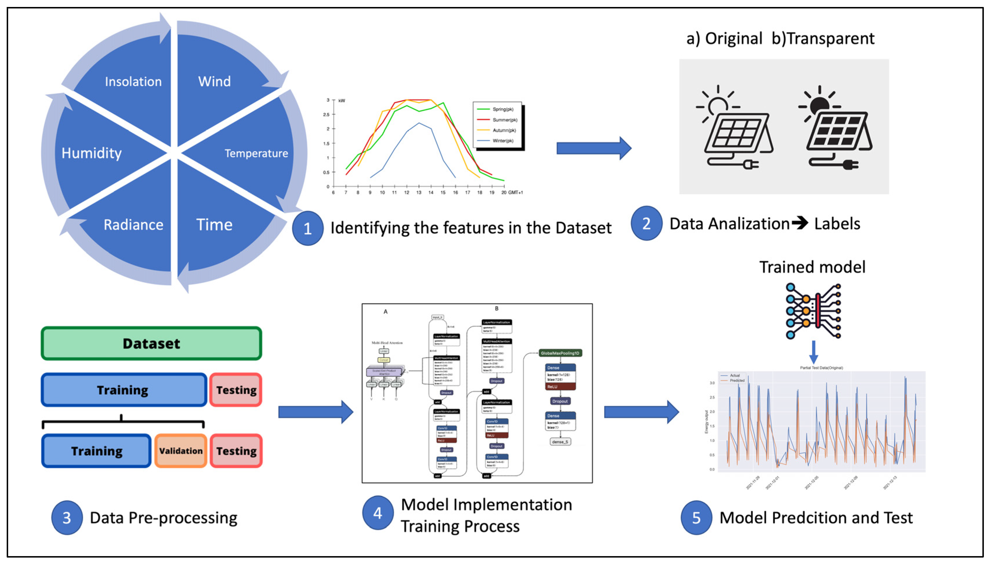
The overall workflow of the power generation forecasting system is described in Figure 5. In this work, the pre-processing stage required observation of the collected dataset to analyze all dependent variables. Dependent variables as features are wind, humidity, temperature, solar radiance, solar insolation, and time. In the second step, the data divided into two parts as collected two target variables (label) from non-transparent and transparent type solar modules. Afterward, thoroughly inspecting the raw dataset, the pre-processed dataset was split into training and test subsets in random shifted order. Furthermore, the training subset feeds into the model for the training process and accuracy results obtained on the test dataset.

3. Results and Discussions

3.1. Performance Evaluation

Transformer models have shown state-of-the-art performance on many time series forecasting problems [22,23]. To evaluate the effectiveness of the proposed method, experiments were conducted using one year of data (from 1 January to 31 December 2021) from NewREC located in Buan-gun, Republic of Korea. For each day, data were collected only during daylight hours, from 5 am to 7 pm. The original PV data is collected at one-hour intervals. Upon completion of the prediction process on the test dataset, the result is compared with the actual and predicted values with implemented Deep Learning models, including LSTM, GRU, and Transformer models.
To evaluate the accuracy of the implemented model on the test dataset, we utilized MAE as the loss function and RMSE and MSE as accuracy metrics, as these are the primarily used metrics in the time-series models. These metrics provide a good summary of the model’s capability to make a prediction on unseen data.
The loss function can be expressed as:
MAE = i = 1 n | y i y i ^ | n
where y i is the actual value and y i ^ is the predicted one. The mean absolute error MAE is the average of the absolute errors between the predicted and actual values, reflecting the actual predicted error. The lower the error value, the better the model.
Two coefficients used to assess the accuracy of predictive models are presented in formulas (4) and (5), respectively:
MSE = 1 n i = 1 N ( y i y i ^ ) 2
where N is the number of observed samples, y i is the actual number, and y i ^ is the predicted value by the model. The essence of the metric is to minimize the sum of squared deviations of the actual values from the predicted ones (Sum of Squared Errors).
RMSE = i = 1 N ( y i y i ^ ) 2 N
RMSE error is simply the square root of the MSE error. Unlike MSE, it has the same units as the original values of the dataset. As a result, it also operates with smaller absolute values and has a faster computation time.
Table 2 presents the overall metrical results of the implemented models (traditional RNN models-LSTM, GRU, and Transformers) for non-transparent and transparent solar panels. Additionally, the accuracy results of traditional RNN models-LSTM and GRU, and our best implemented Transformer model summarized in terms of MSE, MAE, and RMSE values. It is seen that the implemented Transformer model outperforms the other two models in terms of the accuracy of forecasted values.

3.2. Visualization Results

Upon completion of the training process, the result is compared with the actual values of the test dataset. We visualized the test results of the implemented Transformer model in Figure 6 and Figure 7 for both Transparent and non-Transparent module types, respectively. Figures show the actual hourly generated electricity compared to the forecasting models’ predictions. We can observe that forecasts match the actual data, particularly in the winter season, when the system does not generate much power.

3.3. Feature Importance

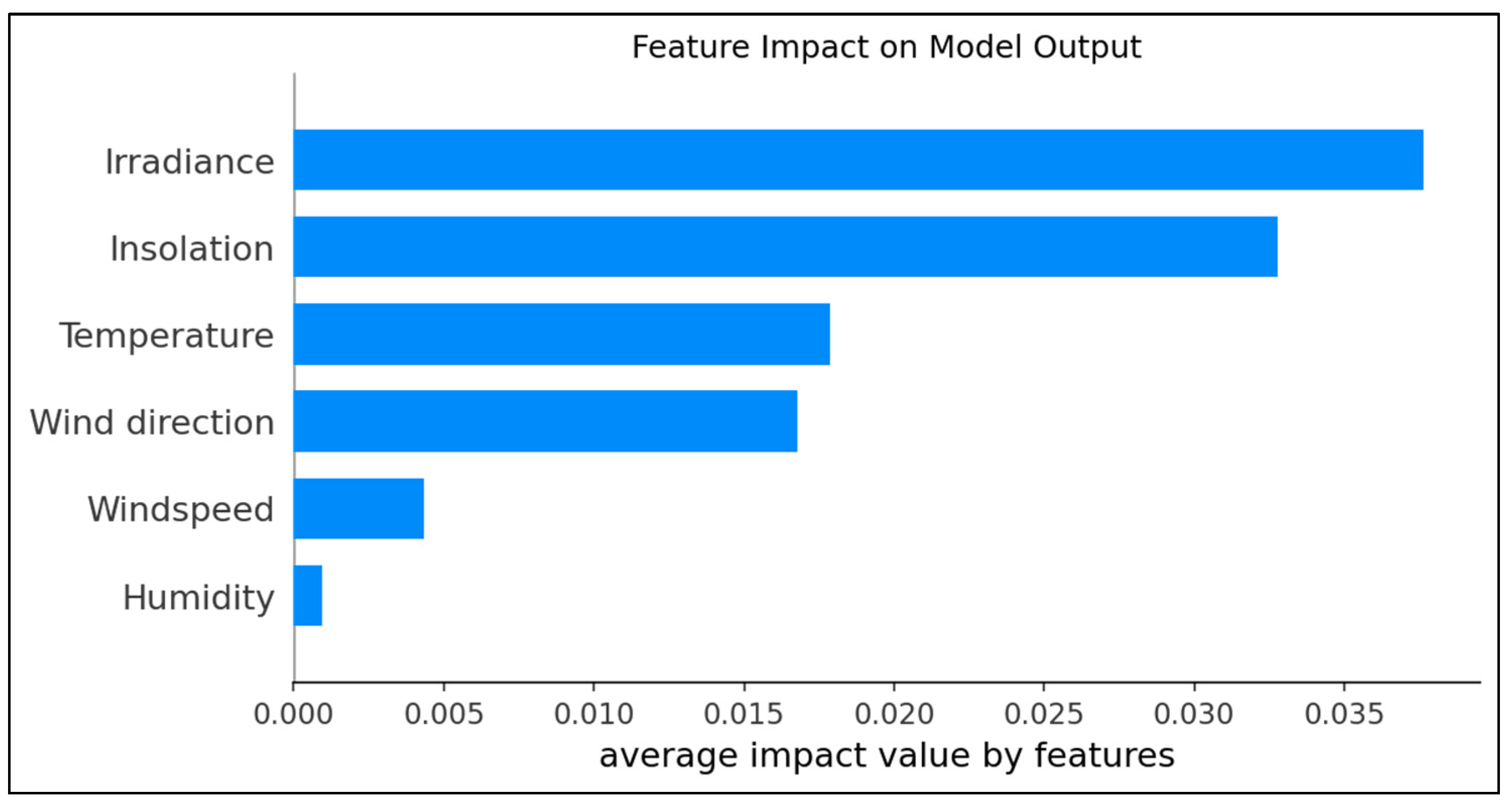
In our dataset, we have six features to train our model. The followings are temperature, wind speed, wind direction, humidity, irradiance, and insolation. It is a well-known fact that not all dataset features will equally impact the performance of the trained model. Therefore, determining which features have the most predictive power is another critical step in model-building. A higher score on the feature means a more significant effect on the model`s ability to predict target variables.
Figure 8 demonstrates the average impact value of each feature of our dataset. The top three features with the highest impact are irradiance, insolation, and temperature. By analyzing this data, one can understand the relationship between the features and target variables. In support, the low impact features on the model can be deleted after checking the relationship with variables. As a result, the model would become lighter and increasing the speed the model’s prediction of the target variables.
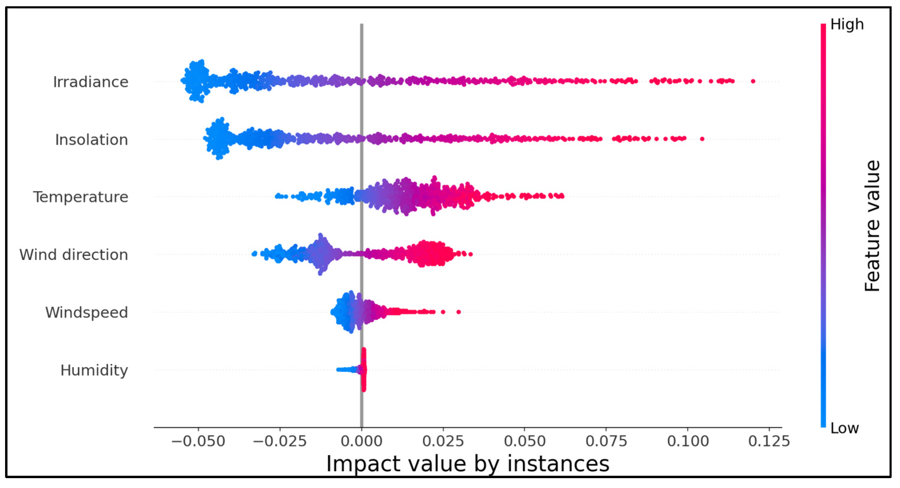
To further analyze the impact score of each feature, each instance of the test dataset on the model’s performance using SHAP [24] values have been observed. Figure 9 demonstrates the feature importance analysis of all 708 instances of the test dataset. As mentioned above, the most critical features are irradiance, insolation, and temperature, and most of their instances positively affect the prediction ability of the model. However, it can be seen that some of the instances are negative numbers, which means the overall accuracy loss.

4. Conclusions

This research presents a method for predicting the PV power generation of photovoltaic stations in eastern part of Korea by the Transformers algorithm. The original dataset for deep learning models is obtained from the target value of electricity generation in kWh and other features, such as weather conditions, solar radiance, and insolation. All PV power generation data were collected from two operational PV panels, such as non-transparent and transparent solar panels. Deep learning models with time series algorithms were designed to forecast the hourly PV power generation of non-transparent and transparent solar panel systems. The study results show that the developed predictive model has a mean absolute error (MAE) of approximately 0.18 kWh and 0.17 kWh for both non-transparent and transparent type modules over the predicted interval. The root mean square error of the model (RMSE) is 0.24 kWh and 0.21 kWh, respectively. The developed model makes it possible to increase the efficiency of the operation of photovoltaic stations and reduce economic losses. In addition to a higher power generation capability, the transparent module is less prone to be heated up, making it possible to do without cooling devices and lowering the cost of building a solar system overall. Moreover, we can further improve the predictive model to reduce the prediction error by considering accumulated experience, more detailed analysis of the input data, and precisely tuning neural networking layers.

Author Contributions

Conceptualization, J.S. and M.S.A.; methodology, J.S.; software, J.S.; validation, J.S., J.P., and M.S.A.; formal analysis, J.S.; investigation, J.S..; resources, J.S., J.P., and M.S.A.; data curation, J.S.; writing—original draft preparation, J.S.; writing—review and editing, J.S., O.-B.Y., and M.S.A.; visualization, J.S.; supervision, M.S.A.; project administration, O.-B.Y.; funding acquisition, M.S.A. All authors have read and agreed to the published version of the manuscript.

Funding

This research received no external funding.

Data Availability Statement

Raw data were generated at NewREC, Buan-gun, Republic of Korea. Derived data supporting the findings of this study are available from the corresponding author on request.

Acknowledgments

This work was supported by the “Human Resources Program in Energy Technology” of the Korea Institute of Energy Technology Evaluation and Planning (KETEP), granted financial resource from the Ministry of Trade, Industry and Energy, Republic of Korea (No. 20204010600470). This work was also supported by the National Research Foundation of Korea (NRF) grant funded by the Korea government (MSIT). (Project No. 2022M3J7A1066428).

Conflicts of Interest

The authors declare no conflict of interest.

References

  1. Halkos, G.E.; Gkampoura, E.C. Reviewing usage, potentials, and limitations of renewable energy sources. Energies 2020, 13, 2906. [Google Scholar] [CrossRef]
  2. Reindl, T.; Walsh, W.; Yanqin, Z.; Bieri, M. Energy meteorology for accurate forecasting of PV power output on different time horizons. Energy Procedia 2017, 130, 130–138. [Google Scholar] [CrossRef]
  3. Hayat, M.B.; Ali, D.; Monyake, K.C.; Alagha, L.; Ahmed, N. Solar energy—A look into power generation, challenges, and a solar-powered future. Int. J. Energy Res. 2019, 43, 1049–1067. [Google Scholar] [CrossRef]
  4. Sampaio, P.G.V.; González, M.O.A. Photovoltaic solar energy: Conceptual framework. Renew. Sustain. Energy Rev. 2017, 74, 590–601. [Google Scholar] [CrossRef]
  5. Sağlam, Ş. Meteorological parameters effects on solar energy power generation. WSEAS Trans. Circuits Syst. 2010, 9, 637–649. [Google Scholar]
  6. Kabir, E.; Kumar, P.; Kumar, S.; Adelodun, A.A.; Kim, K.H. Solar energy: Potential and future prospects. Renew. Sustain. Energy Rev. 2018, 82, 894–900. [Google Scholar] [CrossRef]
  7. Choi, B. ARMA Model Identification; Springer Science & Business Media: Berlin/Heidelberg, Germany, 2012. [Google Scholar]
  8. Shumway, R.H.; Stoffer, D.S. Time series regression and ARIMA models. In Time Series Analysis and Its Applications; Springer: New York, NY, USA, 2000; pp. 89–212. [Google Scholar] [CrossRef]
  9. Gardner, E.S., Jr. Exponential smoothing: The state of the art. J. Forecast. 1985, 4, pp. 1–28 doiorg/101002/for3980040103. [Google Scholar] [CrossRef]
  10. Gurney, K. An Introduction to Neural Networks; CRC press: Boca Raton, FL, USA, 2018. [Google Scholar] [CrossRef]
  11. Drucker, H.; Burges, C.J.; Kaufman, L.; Smola, A.; Vapnik, V. Support vector regression machines. In Advances in Neural Information Processing Systems 9; MIT Press: Cambridge, MA USA, 1996. [Google Scholar]
  12. Martínez–Álvarez, F.; Troncoso, A.; Riquelme, J.C.; Aguilar–Ruiz, J.S. LBF: A labeled-based forecasting algorithm and its application to electricity price time series. In Proceedings of the 2008 Eighth IEEE International Conference on Data Mining, Pisa, Italy, 15–19 December 2008; IEEE: Piscataway, NJ, USA, 2008; pp. 453–461. [Google Scholar] [CrossRef] [Green Version]
  13. Sherstinsky, A. Fundamentals of recurrent neural network (RNN) and long short-term memory (LSTM) network. Physica D Nonlinear Phenom. 2020, 404, 132306. [Google Scholar] [CrossRef]
  14. Vaswani, A.; Shazeer, N.; Parmar, N.; Uszkoreit, J.; Jones, L.; Gomez, A.N.; Kaiser, Ł.; Polosukhin, I. Attention is all you need. In Proceedings of the 31st Conference on Neural Information Processing Systems (NIPS 2017), Long Beach, CA, USA, 4–9 December 2017; Volume 30. [Google Scholar] [CrossRef]
  15. Wu, N.; Green, B.; Ben, X.; O’Banion, S. Deep transformer models for time series forecasting: The influenza prevalence case. arXiv 2020, arXiv:2001.08317. [Google Scholar] [CrossRef]
  16. Wu, S.; Xiao, X.; Ding, Q.; Zhao, P.; Wei, Y.; Huang, J. Adversarial sparse transformer for time series forecasting. Adv. Neural Inf. Process. Syst. 2020, 33, 17105–17115. [Google Scholar]
  17. Wolf, T.; Debut, L.; Sanh, V.; Chaumond, J.; Delangue, C.; Moi, A.; Cistac, P.; Rault, T.; Louf, R.; Funtowicz, M.; et al. Transformers: State-of-the-art natural language processing. In Proceedings of the 2020 Conference on Empirical Methods in Natural Language Processing: System Demonstrations, Online, 16–20 November 2020; Association for Computational Linguistics: Cedarville, OH, USA, 2020; pp. 38–45. [Google Scholar] [CrossRef]
  18. Devlin, J.; Chang, M.W.; Lee, K.; Toutanova, K. Bert: Pre training of deep bidirectional transformers for language understanding. arXiv 2018, arXiv:1810.04805. [Google Scholar] [CrossRef]
  19. Hochreiter, S.; Schmidhuber, J. Long short-term memory. Neural Comput. 1997, 9, 1735–1780. [Google Scholar] [CrossRef] [PubMed]
  20. Chung, J.; Gulcehre, C.; Cho, K.; Bengio, Y. Empirical evaluation of gated recurrent neural networks on sequence modeling. arXiv 2014, arXiv:1412.3555. [Google Scholar] [CrossRef]
  21. Available online: https://towardsdatascience.com/the-fall-of-rnn-lstm-2d1594c74ce0 (accessed on 25 September 2022).
  22. Grigsby, J.; Wang, Z.; Qi, Y. Long-range transformers for dynamic spatiotemporal forecasting. arXiv 2021, arXiv:2109.12218. [Google Scholar] [CrossRef]
  23. Zhou, H.; Zhang, S.; Peng, J.; Zhang, S.; Li, J.; Xiong, H.; Zhang, W. Informer: Beyond efficient transformer for long sequence time-series forecasting. In Proceedings of the AAAI Conference on Artificial Intelligence, Online, 2–9 February 2021; Curran Associates, Inc.: Red Hook, NY, USA, 2021; Volume 35, pp. 11106–11115. [Google Scholar] [CrossRef]
  24. Lundberg, S.M.; Lee, S.I. A unified approach to interpreting model predictions. Adv. Neural Inf. Process. Syst. 2017, 30. [Google Scholar] [CrossRef]
Figure 1. Real photographs of (A) Non-transparent and (B) Transparent Photovoltaic Modules.
Energies 16 01353 g001
Figure 2. Generation of Solar Energy on hourly basis from both non-transparent and transparent type solar modules.
Energies 16 01353 g002
Figure 3. The features of the dataset: Irradiance, Humidity, Temperature, Insolation, and Windspeed, with their average values.
Energies 16 01353 g003
Figure 4. The architecture of implemented Transformer model. (A) Multi-Head Attention structure. Original paper: [14], (B) Implemented Network Architecture.
Energies 16 01353 g004
Figure 5. General workflow of the implemented system.
Energies 16 01353 g005
Figure 6. Transformers model test result visualization of Transparent type module.
Energies 16 01353 g006
Figure 7. Transformer model test result visualization of not-transparent type module.
Energies 16 01353 g007
Figure 8. Impact of feature on overall performance of the Transformers model.
Energies 16 01353 g008
Figure 9. Feature impact by instance of the test dataset on model’s performance.
Energies 16 01353 g009
Table 1. Physical characteristics of PV modules.
TypeNon-TransparentTransparent
Module output400 W405 W
Module size2039 × 1001 × 40 mm2039 × 1001 × 40 mm
Module weight22.2 kg22 kg
Table 2. Evaluation metric results for Non-Transparent and Transparent modules.
Non-Transparent ModuleTransparent Module
Model/MetricsMSEMAERMSEModel/MetricsMSEMAERMSE
LSTM0.0700.2170.27LSTM0.0570.190.23
GRU0.6570.2100.26GRU0.0520.180.22
Transformers0.0570.1870.24Transformers0.040.170.21
Disclaimer/Publisher’s Note: The statements, opinions and data contained in all publications are solely those of the individual author(s) and contributor(s) and not of MDPI and/or the editor(s). MDPI and/or the editor(s) disclaim responsibility for any injury to people or property resulting from any ideas, methods, instructions or products referred to in the content.