Article

A Deep Learning Approach for Exploring the Design Space for the Decarbonization of the Canadian Electricity System

1
Institute for Integrated Energy Systems, University of Victoria, Victoria, BC V8P 5C2, Canada
2
Department of Civil Engineering, University of Victoria, Victoria, BC V8P 5C2, Canada
3
Department of Computer Science, University of British Columbia, Vancouver, BC V6T 1Z4, Canada
*
Author to whom correspondence should be addressed.
Energies 2023, 16(3), 1352; https://doi.org/10.3390/en16031352
Submission received: 5 January 2023 / Revised: 23 January 2023 / Accepted: 25 January 2023 / Published: 27 January 2023

Abstract

:
Conventional energy system models have limitations in evaluating complex choices for transitioning to low-carbon energy systems and preventing catastrophic climate change. To address this challenge, we propose a model that allows for the exploration of a broader design space. We develop a supervised machine learning surrogate of a capacity expansion model, based on residual neural networks, that accurately approximates the model’s outputs while reducing the computation cost by five orders of magnitude. This increased efficiency enables the evaluation of the sensitivity of the outputs to the inputs, providing valuable insights into system development factors for the Canadian electricity system between 2030 and 2050. To facilitate the interpretation and communication of a large number of surrogate model results, we propose an easy-to-interpret method using an unsupervised machine learning technique. Our analysis identified key factors and quantified their relationships, showing that the carbon tax and wind energy capital cost are the most impactful factors on emissions in most provinces, and are 2 to 4 times more impactful than other factors on the development of wind and natural gas generations nationally. Our model generates insights that deepen our understanding of the most impactful decarbonization policy interventions.

1. Introduction

Global greenhouse gas emissions (GHGs) must reach net-zero by 2050–2070 to limit warming to well below 2 °C in alignment with the Paris climate agreement [1] to prevent further escalation of the climate crisis. Decarbonization of the energy system, across all sectors, can be accelerated through the adoption of new technologies and policies across all sectors [2], with the ultimate goal of transitioning the energy system from fossil fuel reliance to sustainable and low-carbon energy sources.
Decarbonization of the power system is central to the decarbonization of the entire energy system. This is because many fossil fuel displacement technologies are electrified devices that rely on electricity, and they will not achieve significant emissions reductions if the electricity they use is generated from high-carbon sources.

1.1. Modelling the Energy System Transition

Energy Systems Models (ESM) are widely used by researchers and engineering analysts to analyze complex and interrelated technical, socio-economic, and spatiotemporal factors in the energy sector [3]. These models are particularly useful for assessing the viability of energy systems, such as the electricity sector, to meet energy demand [4,5]. Conventional ESMs for the electricity sector are typically based on established principles in the field, such as power systems engineering and economics, to optimize technically feasible systems for the least-cost. Then, the insights gained from these models are used by decision-makers and policy analysts to explore alternative pathways and design and evaluate policy related to the energy system [6].
Decision-makers require holistic insights to effectively and accurately evaluate system-level policy responses in a timely manner. However, conventional ESMs are limited in their ability to provide holistic analysis due to the high computational load required to simulate scenarios of transformative systemic change, such as those needed to achieve GHG targets or climate stabilization. These limitations are further compounded when comparing multiple scenarios, making it difficult to identify high-level interactions within the system for policy planning. For example, ESMs are not able to directly quantify the generalized effect of an input parameter (e.g., price of wind energy) on a target output variable (e.g., carbon emissions). Instead, many scenarios must typically be run to search for a trend. Conducting comprehensive sensitivity analyses to assess the robustness of findings is often computationally infeasible.
Therefore, there is a need to improve ESM methods to support the attainment of Canada’s considerable decarbonization obligations by allowing for the prediction of the complex relationships within key sectors and linkages to the broader socio-economic landscape [7,8]. Increasing the computational efficiency of ESMs enables the generation of broader, deeper, and more relevant quantifiable insights delivered by modelling a much wider range of scenarios. A computationally efficient ESM:
  • Facilitates the development of robust, well-supported policy options, including identification of the most critical policy-planning inputs.
  • Provides insights into critical relationships within the energy system design space that would have been previously inaccessible using conventional ESMs, altering the nature of decarbonization conversations, and allowing for large-scale and impact-ranked policy assessment.
We demonstrate that the creation of a novel type of ESM based on surrogate modelling techniques using machine learning (ML) can achieve these goals.

1.2. Literature Review

When an engineering model is computationally expensive for a particular research objective, surrogate modelling techniques can be used to create a lower computational burden statistical model that accurately mimics the behavior of the base model. The ML-based surrogate is trained on a data set containing inputs and outputs from the original model, followed by validation. This surrogate model can then be used to predict the outputs for a large number of input sets quickly, without the need for extensive computational recourses. This significant reduction in required resources enables design space exploration by widening the scope of the design phase, sensitivity analysis, uncertainty analysis, and singular- or multi-objective optimization [9,10].
Surrogate models have been deployed in a variety of engineering disciplines, but their use in describing energy systems is a relatively new area with significant potential. Successful implementation of surrogate techniques have been reported in the context of building energy system models [9]; ML techniques are widely used in this field for creating efficient models, reducing computational cost, and providing faster predictions [11].

Machine Learning for Energy Systems Analysis

ML techniques have been shown to be effective in exploring a wide range of design options and scenarios for energy systems [7]. Provided the training data set is adequately populated in the region of the chosen input values, scenarios involving any combination of chosen input parameter values can be quickly examined without the need for specialized resources. Other ML methods such as classification [12], clustering [13], and outlier detection [14] are capable of extracting similarities and outliers, as well as clustering the results and their input features based on the objective of the problem. Classification methods provide the model with the ability to accurately predict the class of a label for unseen instances of data [15], clustering methods group unlabeled examples based on their similarities and outlier detection methods identify abnormal data. Examples of these techniques in energy systems include the classification of power quality distribution at power system frequency and out of power system frequency [16], outlier detection for identification of abnormally high or low energy use in a building [17], and automatic identification of operational cycles and patterns within complex building energy system [18].
Several studies have demonstrated the power of ML methods in representing energy systems by imposing minimal assumptions on the historical or synthesized data, allowing the extraction of complicated patterns that are difficult to explain mathematically from physical principles. Mosavi et al. [7] reviewed publications that have used various supervised learning methods for a wide range of applications in renewable energy systems and planning. Many of the works reviewed confirmed the ability of supervised algorithms, specifically neural networks (NNs), to extract complex features from a batch of examples in the energy systems context. Zhang et al. [19] compared a collection of ML algorithms as surrogate models for electrical and heating networks with the objective of integrating renewables into the Dutch energy system. Their results showed that the linear regression model and the long short-term memory model had the highest performance the best in each electrical and heating network. Sciazko [20] implemented various interpolation techniques and NN architectures to develop surrogate models for a steam energy network, resulting in the generalization of features of different types of surrogate models and the use of a surrogate model for optimization with a genetic algorithm. Kim et al. [21] employed NN to predict energy consumption in an actual building’s air conditioning system. The model developed in this study enabled forecasting energy consumption with limited variables. The authors reported relatively high accuracy but acknowledged that a sufficient amount of data and model improvement were necessary to achieve even higher accuracy. Uselis et al. [22] studied the use of localized convolutional neural networks for geospatial wind forecasting. They compared the recent state-of-the-art spatiotemporal prediction models on the same data and concluded that convolutional layers can be extended with localization. Harrison-Atlas et al. [23] used an ML technique, namely boosted regression trees, for spatially-explicit prediction of capacity density advances geographic characterization of wind power potential. The study’s findings indicated that this methodology could improve the characterization of spatial aspects of technical potential, a critical element in delivering reliable and actionable conclusions from renewable energy scenarios. Antonopoulos et al. [24] conducted a review of the use of artificial intelligence approaches to model energy demand response with the aim of cost-effectively enhancing the flexibility and reliability of energy systems. This review outlines directions for future research in this rapidly growing area by discussing the advantages and potential limitations of artificial intelligence/ML techniques for different demand response tasks. Ahmad and Chen [15] review the ML forecasting growth and their real-time applications in various energy systems. The authors conclude that supervised learning approaches are suitable for regression problems, like short-term load and price forecasting. NNs also have a wide range of applications in the decarbonization of energy systems, such as decreasing carbon emissions and enhancing energy storage. One example of their successful use is in the efficient and reliable utilization of lithium batteries. In addition to serving as the primary storage method for a decarbonized power system, batteries also hold a significant role in the process of decarbonization [25].
This study builds upon previous successes in using surrogate modelling and ML techniques to represent complex energy systems. The goal is to develop a computationally efficient large-scale electricity system planning ESM that can provide holistic insights and support the attainment of decarbonization goals.

1.3. Objectives and Contributions

The objectives of this research are as follows:
  • To develop a computationally efficient ESM to investigate complex relationships within the Canadian electricity system.
  • To leverage the expanded functionality of this modelling approach to produce high-impact insights into key drivers of Canada’s decarbonization pathways.
To achieve the objectives of this research, we propose a method to explore the Canadian electricity system design space using an ML surrogate of the Canadian Opportunities for Planning and Production of Electricity Resources (COPPER) model [8]. With a computationally efficient model emulating the results of COPPER, complex relationships within the electricity system are comprehensively explored, by pulling out emergent trends over thousands of optimal solutions allowing for the identification of key factors, clustering input-output correlations, and quantification of sensitive design variables. This effort ultimately supports more evidence-based dialogue and informed policy for rapid national-scale decarbonization.
Many of the successful applications of ML to renewable energy systems have focused on analysis with a narrower scope, such as a single technology, sector, or geographical region [7]. To the best of our knowledge, there is not yet any tool that utilizes ML methods to investigate the complex interdependency of factors involved in large-scale energy systems and the efficacy of sustainable energy policies Therefore, the contributions of this work are as follows:
  • We propose a pipeline that utilizes ML methods to reduce the computational burden of a capacity expansion model at a national level by 5 orders of magnitude, with a mean R-squared value of 0.93. Utilizing this tool, we investigate the complex interdependency of factors involved in large-scale energy systems and the efficacy of sustainable energy policies.
  • Using this model, we identify key variables affecting power systems and provide sensitivity measures leading to a more robust analysis.
  • We implement an easy-to-interpret method utilizing an unsupervised ML method and comparative maps, allowing for the effective conveyance of results to stakeholders.
  • We compare the outputs’ behavior to changes in all inputs. The impact of all inputs on specific outputs is evaluated with a quantitative metric.
  • The results of this study contribute a huge number of insights into Canada’s electricity system development, some of which are further explored and understood through advanced visualizations.
This paper has been divided into 6 sections. Section 2 elaborates on our methodology in utilizing ML methods for exploring the vast design space. In Section 3.1, the performance of the surrogate model is assessed in terms of accuracy, speed, and memory usage relative to the base COPPER model. Then in Section 3.2, the results are visualized to qualify and quantify the correlations of policy-relevant inputs to emergent system outputs, allowing for the identification of key factors driving emissions and wind and natural gas (gas) generation capacity. The results of the model development process and the ensuing analysis are then summarized, and the implications of this work are discussed in Section 4.

2. Materials and Methods

In this work, we employed NNs as a surrogate modelling technique to describe the Canadian electricity system.

2.1. Electricity System Capacity Expansion Modelling Using COPPER

COPPER is a recently developed long-term planning model that determines the least-cost generation and transmission capacity mix over a specified period and timestep. This calculation is based on a predefined set of inputs including projected demand, geographical wind, and solar resource distributions, and modelled policies. COPPER was designed to address research questions regarding various Canadian capacity expansion scenarios using an objective function that minimizes total costs under technical power system constraints, simulating across time steps to chart effective pathways. Scenarios can then be compared through visualizations. It was chosen as the base model for this analysis due to its inclusion of major carbon management policies aimed at reaching Canada’s goal of net-zero emissions. The version of COPPER used in this work includes a carbon tax, coal power phase-out, and gas-fired power plant performance standards.
COPPER is a powerful tool, and this scenario-based analysis method has been used to evaluate and compare the effects of distinct carbon pricing options on the future generation mix [8]. However, COPPER’s framework is computationally intensive and impractical for isolating, quantifying, or ranking the impact of a carbon tax or other important policy parameters relative to other design variables. Running a single scenario can require 16 to 32 CPUs, 64 to 132 GB of memory, and 11–72 h of computing time. To address this issue, this work applies surrogate modelling techniques to the COPPER model to make it more efficient for exploring research questions related to input sensitivities in the Canadian climate policy design space. This includes the effects of altering technology costs through subsidies, carbon tax values, and demand growth through efficiency regulations on emissions and generation capacity.

2.2. Surrogate Model Development with Deep Neural Networks

A NN is a parametric function that transforms an input into a corresponding output by utilizing stacked layers of linear parametric transforms combined with nonlinear “activation” functions between the layers. Theoretically, NNs can model any base function with enough parameters [26], including complex mappings between inputs and outputs exhibited by energy systems models, with reasonable computation time and high accuracy [27,28].
NNs with more than two layers are referred to as deep NNs, and each added layer allows the NN to capture more complex mappings. Among the various deep NN architectures introduced in literature [29], residual networks have gained popularity for their performance and ease in training. The core feature of residual networks is the existence of residual (skip) connections between various layers, which enables the NN to learn more intricate relationships [30]. This is particularly crucial when attempting to model complex interdependencies within the electricity system over time, as represented by the COPPER model.
A typical training procedure involves providing a deep network with paired inputs and corresponding outputs. The parameters of the NN are then optimized via gradient-based learning [26] to minimize the discrepancy between the deep network outputs and the supplied outputs. The optimization process typically involves selecting a random subset of the training data, called the training batch, and an optimization process, such as ADAM [26], that is specifically designed for NN training. We followed standard protocols for deep NN training, as outlined in [27].

2.3. COPPER Surrogate Model Development

The model development was carried out in three phases: (1) data generation, (2) data preparation, and (3) model training.

2.3.1. Data Generation

To train, validate, and test the surrogate NN options, a dataset of COPPER simulations was generated. In this analysis, the carbon tax, capital costs by generation type, and annual demand growth rate by province were selected as the most important design inputs based on optimization constraints in COPPER [8]. These variables represent possible Canadian climate policy pathways; specific carbon tax values, technology subsidies, efficiency regulations, and demand-side interventions. These variables were initially sampled uniformly over predefined ranges listed in Table 1.
The lower and upper bounds for each input were determined in consultation with subject matter experts considering the feasible ranges for policy tuning based on values taken from the paper proposing CREST [31] and COPPER [8]. We increased these values by approximately 25% for the upper bounds and decreased by approximately 25% for the lower bounds, which is a common practice in sensitivity analysis to cover the whole design space. A carbon tax range was selected based on the minimum and maximum increase in each year present in scenarios developed for COPPER [8], which encompasses Canada’s “A Healthy Environment and a Healthy Economy” (HEHE) [32] carbon pricing plan. Capital costs are location-specific and exhibit wide variability between studies, so the ranges selected for this analysis were also based on values taken from the papers proposing CREST [31] and COPPER [8]. The ranges for capital costs of wind and solar were chosen to be wider than in [8] in consideration of the uncertainty in the technological evolution of these renewable energy sources and covering the design space. Demand growth varies between provinces and was taken from [8,31], and it was also widened by 25% on either side of the nominal value. In COPPER V5 was used in this work, and capital costs and capacity factors are considered constant in each year. This work does not account for technological evolution over time is not accounted for, adding a limitation to the validity of this work.
Next, complete input datasets including the randomly sampled values of the design inputs were used to generate COPPER simulation output datasets. Given the long duration required for COPPER runs, the initial sample size was 1000 datasets, each consisting of a full set of COPPER results in 2030, 2040, and 2050. For dataset generation, we applied the default constraints in COPPER. These conditions include the application of the carbon tax to gas prices; consideration of existing transmission between provinces with no interprovincial transmission capacity expansion; consideration of existing hydro generating capacities with no hydro generation capacity expansion. These constraints were selected to encompass the most practical and non-contentious pathways, as the thorough examination of these matters is not the primary focus of this analysis. Additional information on the parameters used in the COPPER model can be found in reference [8].
The training dataset was derived from the COPPER simulation results. Specifically, the annual carbon emissions by province and the capacity for wind and gas at both the provincial and national levels were isolated. These variables were chosen as crucial indicators of interest in policy formulation.

2.3.2. Data Preparation

The data were preprocessed for NN training through cleaning, normalization, and standardization. Firstly, the model outputs were cleaned up by removing the missing values (NaNs), constant values, and the output data outliers based on a 5-sigma margin. Next, outputs were standardized based on their mean and standard deviation, to increase the speed of model training and give equal weight to all the model outputs. Additionally, variance clipping was applied to the model outputs; where values with a standardized variance of less than 0.001 were considered model noise and excluded from the training process. The model inputs were normalized based on their maximum and minimum values such that all inputs are in the range of 0 to 1. The data set of COPPER simulations was generated and split into training (80%), validation (10%), and testing (10%) subsets. Normalization of inputs and standardization of outputs were performed as per eqns. (1) and (2), respectively:
For i in X:
x ^ i = x i m i n ( x i ) m a x ( x i ) m i n ( x i )
For i in Y:
y ^ i = y i m e a n ( y i ) s t d ( y i )

2.3.3. Model Training

The model training algorithm aimed to minimize the loss function, which was defined as mean-squared error (MSE) between the NN output predictions and the provided data (calculated using eqn. (3)). Lower MSE values are indicative of greater model accuracy. To prevent overfitting, the training and validation losses were compared during the model tuning process. The NN architecture was selected based on empirical experimentation, by ensuring that the validation loss did not increase over additional training epochs. The model training platform was developed with the PyTorch Lightning library in Python [33], and it was executed on a Graphics Processing Unit provided by Compute Canada.
M S E = 1 n i = 1 n ( Y i Y i ^ ) 2

2.3.4. Ablation Study to Determine Model Architecture

We experimented with a multi-layered NN architecture featuring residual blocks [30] to regress the model outputs against the training dataset. The key design choices in model architecture are the number of layers and neurons per layer, activation function (sigmoid, ReLu, hyperbolic tangent, etc.), batch size, and learning rate [26]. Dropout was used to reduce the risk of overfitting by random omissions of neurons during a neural network’s training process [34]. A detailed examination of the impact of changes in design parameters on the model’s performance is provided in Table 2, which presents a selection of high-accuracy architectures identified during the experimental process, along with their corresponding prediction errors.
Finally, the model architecture with 12 residual blocks was selected. Each block consists of two linear layers, two batch normalizations, two ReLu activation functions, and two dropout layers. This model is summarized in Table 3, and its architecture schematic is shown in Figure 1.

2.4. Exploring Correlations in the Design Space

The proposed model was used to analyze the design space, quantify correlations between outputs and inputs, and identify key factors affecting model results. Correlations between each input and output were investigated using the COPPER surrogate model. The inputs were randomly sampled 1000 times from a uniform distribution, with one input being varied randomly while the other inputs were kept constant at their respective mean values. The outputs of the surrogate model were then calculated, recorded, and plotted against the chosen input variable. This process generated more than 2000 plots, which collectively illustrate interdependencies between inputs and outputs. Due to the scale of this analysis, a pipeline was implemented to process results effectively and identify key insights. Two analytical and visualization techniques were applied to communicate the findings:
  • Clustering and mapping input-output relationships onto heat maps to provide qualitative depictions of the strength of each correlation.
  • Charting the normalized maximum derivatives of two key outputs in each time step with respect to each input as a supplementary indicator showing the relative quantified impact of all inputs on a target output.

2.4.1. Clustering and Dimensionality Reduction of the Results:

We used clustering and dimensionality reduction techniques to group similar relationships that were found between each input and output. This allowed us to identify strong or surprising correlations among the 2000 plots more efficiently, rather than having to review each one individually.
Clustering is a data analysis technique used to group similar subgroups (clusters) in the dataset. Firstly, we used the K-means algorithm to group data points based on their similarity in terms of shape. This allows us to quantify correlation and identify the key factors that affect the model results. K-means is an unsupervised ML algorithm that iteratively identifies k distinct, non-overlapping clusters within the data set such that each datum can be assigned to a group. The pattern of change (increase, decrease, etc.) in input-output variation can then be identified through observation for each grouping.
After clustering the data, we used visualization techniques to help identify the unique relationship of each group. We used the t-distributed stochastic neighbor embedding (t-SNE) technique [35], which is a dimensionality reduction method that maps the high-dimensional data to a 2D plot, making it easier to visualize and understand the multidimensional clusters. This technique helped us to more easily identify the characteristic relationship of each group.
Then, the characteristic relationships observed within each group were labeled to facilitate the interpretability of the large quantity of information to stakeholders effectively. Eight distinct input-output relationship types were identified, as summarized in Table 4.

2.4.2. Relative Impact of Policy Parameters

To quantify the relative impact of specific input parameters on selected outputs, we employed a mathematical technique known as maximum absolute derivatives of standardized outputs with respect to each normalized input. This method provides a quantitative measure of the relative influence of each input parameter on the selected outputs by determining the peak sensitivity of an output to variations in specific input parameters. Calculation of maximum derivatives is a computationally demanding process that is made feasible using a surrogate model. We chose two outputs, wind and gas capacity over time, for this analysis as they are indicative of successful decarbonization in future energy system capacity expansion. The normalized maximum derivatives for these outputs with respect to all inputs were visualized using bar charts to identify which inputs have the greatest impact on these outputs, thus providing insights on how to achieve decarbonization.

3. Results

The results of this work are presented in two sections. The first section covers the results of the surrogate model development, including the model evaluation, performance, and limitations. The second section presents the results of the analysis that was conducted using the proposed model.

3.1. COPPER Surrogate Model Performance

In this section, we evaluate the results, performance, and computational cost of the surrogate model in comparison to the actual COPPER model and point out the limitations of the surrogate model. This section of the results will help to determine how well the surrogate model approximates the actual COPPER model, and to identify any output where the surrogate model may not be as accurate or efficient as the actual model. This comparison will give an idea about the validity of the proposed model and its limitations.

3.1.1. Model Evaluation

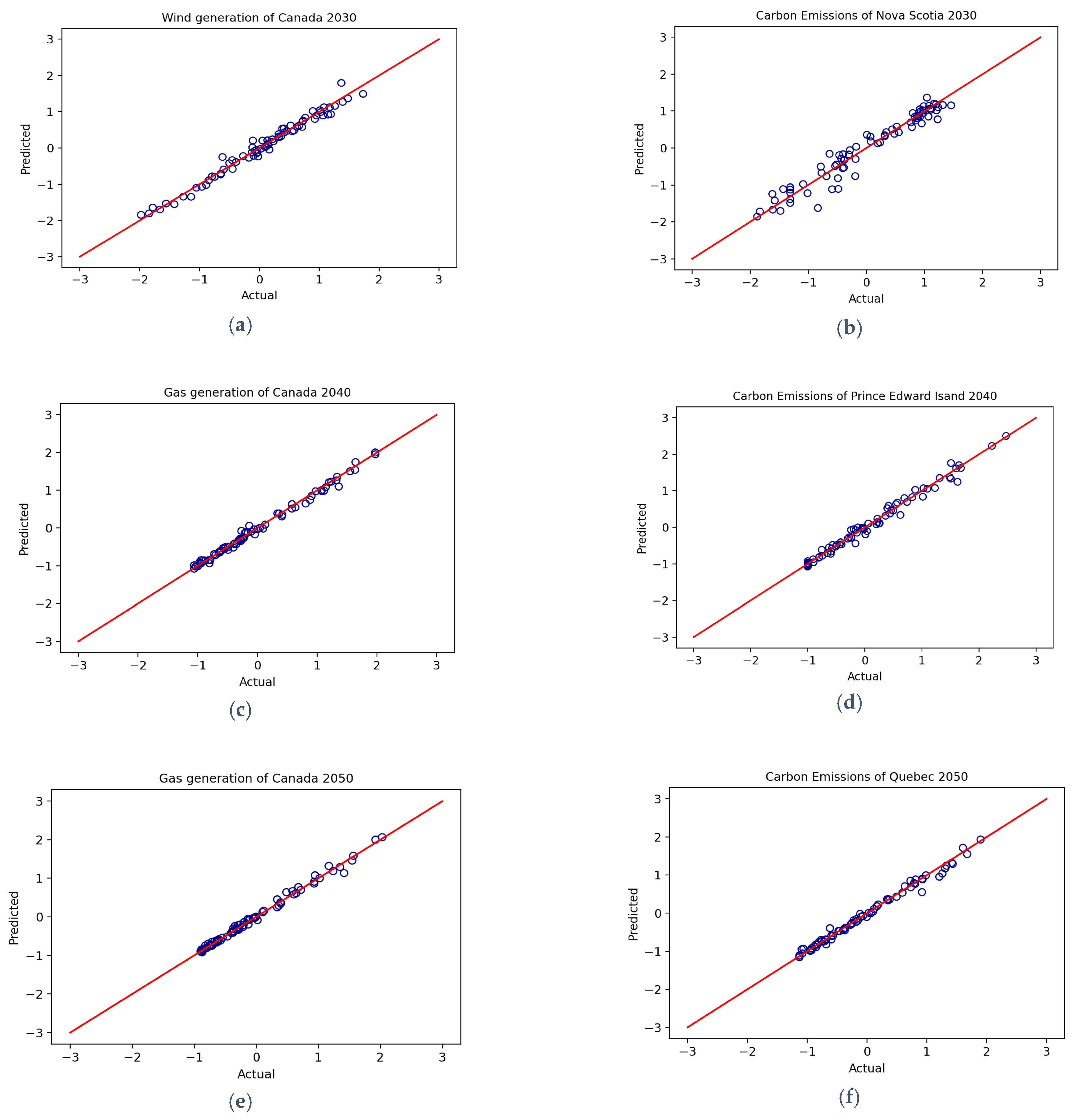
A lower MSE loss generally indicates greater accuracy in predictions during model tuning. However, it is not clear what MSE loss value should be considered a sufficiently close approximation of the base COPPER model. To resolve this, we assess the quality of the output regressions, which means comparing the results of the surrogate model with the actual results of COPPER, to evaluate the quality of the prediction. For each ML model output, we generated a scatter plot for comparison to the same output from the test dataset. An ideal surrogate model would produce diagonal lines with R-squared values of 1 for all plots. As a secondary metric, we report the minimum R-squared value overall output regression plots and set an acceptance threshold of 93%.
Table 5 reports the performance results of the proposed model, including training, validation, and test errors, as well as the R-squared value for the test data set. The R-squared value is a measure of the goodness of fit of the model, with a value of 1 indicating a perfect fit and a value of 0 indicating no fit. For each datum in the test dataset, R-squared is calculated, and then the minimum, maximum, and mean are calculated over the test dataset. This table shows the R-squared distribution statistics with a mean of 0.93 for all regressions. These results give an overall idea of how well the model is performing on various data sets. Figure 2 shows six selected regression plots out of 54 with the minimum, maximum, and mean R-squared for the unseen test data set. These figures demonstrate that even in cases where the R-squared value is low, the model still achieves a high degree of accuracy in its predictions. Note, all values are normalized in the figure to facilitate visualization.

3.1.2. Computational Cost Evaluation

Table 6 compares the run-time and required resources of the proposed model against COPPER to evaluate the computational cost of the model. The results show a significant reduction in computational time and required resources when using the proposed model. These results are important for a wide range of applications, as the reduction in computational time and resources can lead to cost savings and make the model more accessible to a broader range of users.

3.1.3. Limitations of Machine Learning Models for Surrogate Energy Systems Analysis

The developed model is less sensitive to parameters with relatively small nominal values across its variation range. This is because these small values approach zero when the input dataset is normalized, leading to their contribution to the MSE in the network being relatively small. As a result, the relative inaccuracy of small values is not a large driver of network optimization or architecture choices, and it is not captured in an overall accuracy metric. This means that the corresponding prediction accuracy for small-valued outputs may be lower than for larger-valued outputs. This is particularly relevant for parameters where there are small variations between provinces. This limitation should be considered when interpreting the results of the model and when making predictions for small-valued parameters. For example, the annual carbon emissions in Nova Scotia are much lower than in Alberta due to differences in population and the carbon intensity of their power grids. Because the model is less sensitive to small values and variations, the predictions for Alberta will tend to be more accurate than for Nova Scotia. This is a common limitation of ML. To overcome this limitation, one could consider collecting more data specific to Nova Scotia or using different techniques such as weighting the loss function to give more importance to specific regions like Nova Scotia or Alberta.
Another limitation of the surrogate model relates to the wider range of inputs that can be changed in COPPER for the purpose of exploring specific scenarios of interest or adding new constraints. In contrast, this surrogate model is limited to the initial input selection chosen for this work. To address this limitation and the uncertainty associated with future capital costs in future work, the selected variation ranges can be widened such as ±50% instead of ±25%, or the analysis could be preceded by a systematic literature review of capital cost projections that were considered beyond the scope of this analysis.
Furthermore, as COPPER improves and more features are added, the NN will need to be retrained to continue to accurately model the Canadian electricity system, which includes the computational cost of producing and updating the training data and retraining the model. For example, we used COPPER V5 for our model development, in which uncertainty of capital costs is not considered and they are constant for each year, but in the latest version of COPPER technology evolutions are considered and capital costs are not constant. Therefore, this model will need to be retrained and updated as COPPER evolves to ensure its continued accuracy.
There are caveats associated with the analysis conducted in this work relative to standard sensitivity analysis methods:
There is an inherent level of error (correlations aren’t R_squared = 1), so it is unclear to what extent the model can accurately reproduce sensitivities.
The input parameters are varied one-at-time (OAT), and this is not considered suitable for sensitivity analysis for a non-linear system. For a non-linear system, a more appropriate sensitivity analysis method would be global sensitivity analysis, which considers the interactions between inputs and can provide more accurate results.

3.1.4. Limitations Relative to COPPER for Policymakers

Finally, the surrogate modelling methodology used in this work has some limitations relative to the base COPPER model in relevance, intelligibility, and validity.
Firstly, the systematic errors identified above demonstrate that the surrogate model is useful for identifying strong key relationships rather than specific numeric results. So, the base COPPER model is more suitable to use in policy design projects where there are numeric objectives. Similarly, the surrogate is the most successful at capturing large values. This led to it producing the most accurate predictions for larger provinces and limiting its relevance to smaller jurisdictions.
Secondly, due to the comparative nature of this analysis and the use of normalized data to generate model outputs results in analysis where all findings are relative, and no numeric results descriptive of the real system are presented in this work. As such, the surrogate lacks some of the intelligibility of the base model, and the values must be abnormalized to be interpreted in the context of the real system.
Finally, the linear programming method used by COPPER has structural validity that the surrogate does not inherently have, as the deep NN structure of the model does not reflect the structure of the real system. Further validation steps must be taken before results developed using this model are implemented.
Each of these limitations could be addressed by simulating with COPPER to replicate key results found using the surrogate model and validating that the simulation results agree with the surrogate results. Then, these simulation results could be used for detailed and nominal value-based policy planning activities more akin to typical COPPER uses.

3.2. Key Relationships in Canada’s Electricity System Design Space

The use of the surrogate model enabled the evaluation of the changes in system outcomes for variations in policy design inputs in the electricity sector design space. A broad array of insights can be drawn from this analysis about Canada’s mid-term electricity sector decarbonization options, including findings regarding the effects of demand growth, technology costs, and carbon taxes in each province between the present time and end dates corresponding to the Paris Agreement targets.
The analysis firstly presents the relationships in a heat map format where the color corresponds to the nature of the relationship, making it easy to identify the strongest relationships affecting key system indicators at each timestep. This allows for a clear visual representation of the data and facilitates the identification of key relationships. Secondly, the outputs’ maximum derivatives with respect to each input are provided as a quantitative metric for understanding the relative importance of policy-relevant inputs for the capacity expansion of gas and wind generation. This allows for a more in-depth understanding of the impact of different inputs on the electricity sector, providing valuable insights into decision-making and policymaking.

3.2.1. Correlations between Inputs, and Emissions and Generation Output

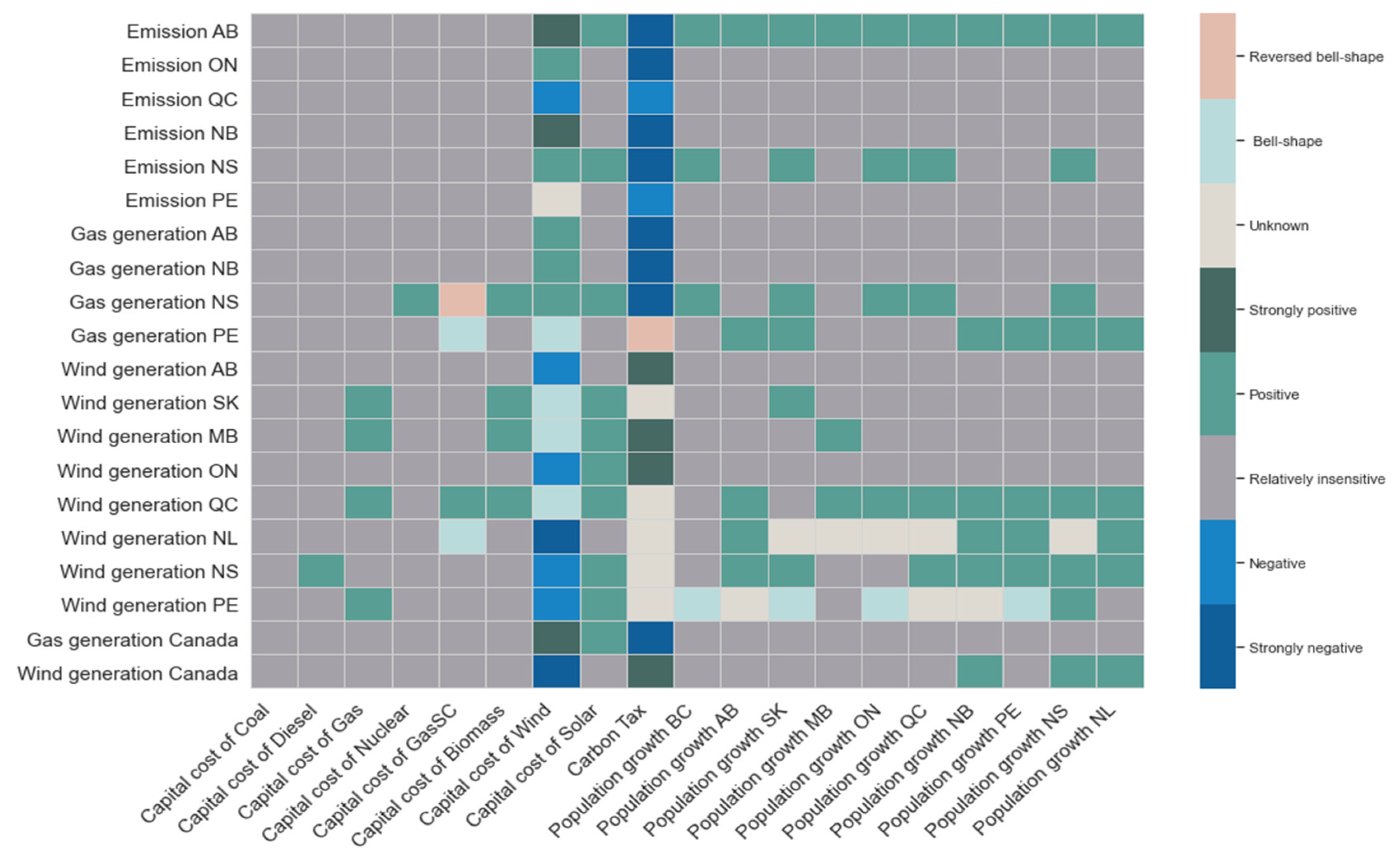
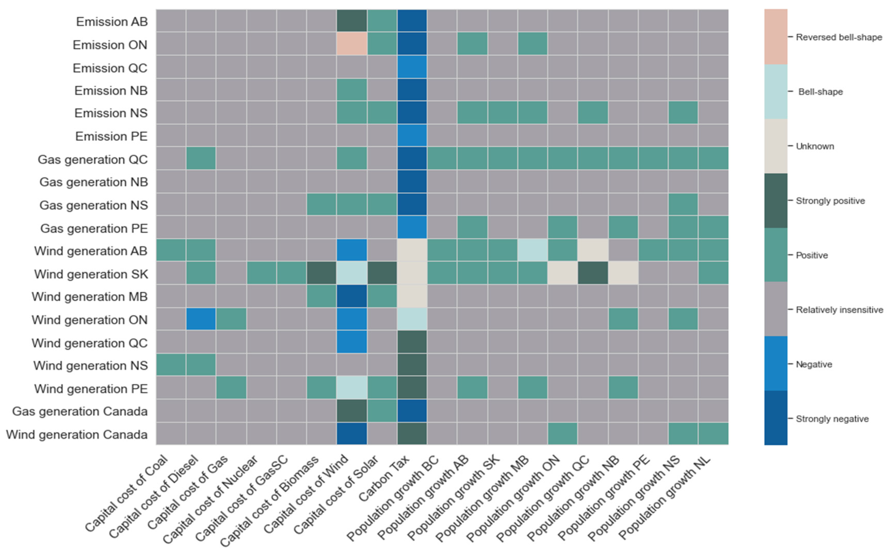
The heat maps depicting the characteristic relationship between each input and each output for the years 2030, 2040, and 2050 are presented in Figure 3, Figure 4 and Figure 5, respectively. They provide a visual representation of how each input affects each output at different timesteps.
The heat map grid size (i.e., the number of input and outputs for which a relationship was classified) vary over the considered timesteps because, as stated above, values that are constant or have very small variations in the training dataset at a timestep were removed from model training process during data preparation based on 5-sigma threshold for standard deviation. In other words, if any selected design output was not associated with relatively significant variation in COPPER simulations, it has been excluded from the surrogate model calculations.
The heat maps present a large amount of information that can be interpreted by analyzing and comparing the pattern of change in output values given variation for each input variable. This clustering can provide valuable insights into the types of relationships between policy inputs and system outcomes. However, the surrogate analysis generates a large amount of information and it would not be feasible to explore every relationship in depth in this work. Therefore, this analysis should be considered as a starting point for further research to identify the most important relationships and their implications.
The results suggest that the carbon tax is the most influential determinant of Canadian electricity system outcomes between now and 2050. The carbon tax level is strongly negatively associated with emissions in most provinces at all time steps. This confirms the importance of Canada’s federal-level commitment to carbon pricing policies, such as the Pan-Canadian Approach to Carbon Pollution Pricing [36].
The results further suggest that wind is the renewable energy source with the greatest influence on Canada’s electricity grid development, particularly for 2030. The capital cost of wind is shown to the positively correlated with emissions in some provinces and negatively correlated with built wind capacity in most provinces. Of all the renewable energy subsidy options, this analysis suggests that reducing the capital cost of wind across Canada results in the greatest emissions reductions. This is a crucial insight for Canada’s 2030 electricity system greenhouse gas targets, as it highlights the importance of reducing the cost of wind energy to achieve emissions reduction goals.

3.2.2. Ranking of Factors Affecting Gas and Wind Capacity Development

In this section, we explore the factors that determine the expansion of gas and wind energy generation capacity at the national scale. These key outcomes do not directly correspond to current Canadian policy targets, such as annual GHG emissions. However, they are responsible for significant contributions to Canadian energy generation and are indicative of either the continuation of business-as-usual or realized decarbonization efforts. By understanding the determinants of these outcomes, policy makers can identify the most effective policies and strategies to promote decarbonization in the Canadian electricity sector.
The analysis of system parameters and their potential impact on the future supply mix in Canada is represented by the maximum derivatives of gas and wind capacities with respect to each input. These values are normalized to determine the relative impact of each variable and are used to rank policy options based on their relative impact. The negative values indicate a negative correlation, positive values indicate a positive correlation, and the absolute value of the maximum derivative represents the strength of the correlation. The results are displayed in bar charts for Canada for the years 2030, 2040, and 2050 in Figure 6, Figure 7 and Figure 8, respectively, which provide a clear visual representation of the relative importance of each input variable in determining the expansion of gas and wind energy generation capacity. This information can help policy makers identify the most sensitive parameters and prioritize efforts to achieve decarbonization goals.
The results reinforce the previously mentioned findings that the most influential determinants of Canadian electricity system outcomes between now and 2050 are the carbon tax and the capital cost of wind. The capital cost of wind plays a particularly significant role, exhibiting a relative impact on the expansion of gas and wind capacities four times as large as any other technology cost. The results show that across all time steps, changes in other demand growth and non-wind energy technology cost parameters have minimal effects on the development of wind and gas generation capacities.

4. Discussion

We find that there is a broad array of holistic insights we can draw from this surrogate model by clustering or by ranking each correlation, and then comparing these relationships across years, provinces, or parameters. The results confirm the effectiveness of policies such as carbon pricing and wind subsidies and highlight their significance compared to other options. The remainder of the analysis will focus on the most notable findings from national-level results.

4.1. Demand Growth Effects

The analysis shows that the relationship between electricity demand and emissions is not consistent across provinces and over time. An increase in demand growth rate will lead to an increase in carbon emissions in most provinces, in New Brunswick and Nova Scotia until 2030 and Alberta until 2040. Of particular interest are the highly positive and positive correlations, respectively, between emissions and gas generation capacity, and demand growth in many of the provinces with the highest populations (i.e., BC, AB, QB) and Nova Scotia. This uneven distribution suggests that policies aimed at addressing future load growth, such as efficiency measures and renewable energy expansion, or increased stringency of renewable portfolio standards over time, should be tailored to the specific needs of each province when implemented at the provincial level.

4.2. Capital Cost Effects

The capital cost of non-renewable energy technologies, including nuclear energy, does not have a significant impact on emissions because carbon pricing is already high enough that non-renewable sources cannot compete with renewable sources in terms of cost. However, the capital costs of solar and wind energy have a significant impact on Canada’s electricity system development and are negatively correlated with emissions and gas capacity in many provinces. This suggests that policies aimed at reducing the cost of renewable energy technologies can effectively reduce reliance on additional gas generation capacity, particularly in New Brunswick and Nova Scotia. Climate policy that raises the capital cost of coal and diesel raises wind capacity in some provinces but also increases gas capacity in other provinces, highlighting the importance of considering localized impacts when implementing federal-level policies like a coal phase-out.

4.3. System Sensitivity over Time

The sensitivity analysis of COPPER, a model used to simulate the electricity sector under a net-zero constraint, shows that the system’s outputs become more stable over time as the grid approaches the net-zero constraint. The greatest variation in emissions and generation mix is seen in 2030, with the impact of changes in demand growth being the highest. By 2040, technology capital costs become less of a determinant of emissions and generation capacities, and the system is less susceptible to diverse outcomes due to changes in parameters. This finding is in line with prior simulations produced using COPPER, which show that carbon-intensive generation (coal, diesel) should be phased out in 2030 to prevent their continued usage into 2050, as their life cycle can be around 20–25 years [8]. This confirms that the most important period for government intervention, decarbonization policies, and green investment is within the next decade.

5. Conclusions

The COPPER model is able to model high-resolution spatiotemporal constraints and detailed policy options, but its computational burden limits its use. The ESM developed in this work addresses this limitation by efficiently exploring the design space for the electricity sector by characterizing the relationships between policy inputs and system outcomes over thousands of model runs. The efficient computational techniques explored in this work have not previously been applied to large-scale ESMs.
The proposed deep NN pipeline outlined in this paper reduced the computational time and required resources by 5 and 6 orders of magnitude, respectively, by only requiring a single CPU while maintaining a high degree of overall accuracy (mean test regression R-squared of 0.93). This addresses the computational limitations of the base COPPER model. The surrogate model was used to produce over 2000 input-output correlation plots, so a visualization method utilizing K-means clustering, comparative heat maps, and ranked bar charts were developed to communicate these insights to diverse stakeholders in an accessible way. This tool allows for easy determination of holistic insights to guide policymakers with quantitative metrics for more effective electricity system decarbonization planning. It has the ability to produce many insights, and in this work, we highlighted the strongest relationships within the system and determinants of key components of the electricity supply mix were highlighted.
The rapid evaluation enabled by this low-burden model allowed for the exploration of new types of research questions and the vast design space for Canada’s electricity system. This analysis revealed that carbon taxes and the capital cost of wind are the most impactful parameters for electricity system outcomes, including emissions reductions, in many provinces. This finding reaffirms and justifies Canada’s commitments to its carbon pricing plan as the most impactful policy measure facilitating the decarbonization of Canada’s electricity sector. Additionally, the analysis revealed that reducing the capital cost of wind is an effective secondary strategy for emissions reduction and research and policy support in this area should be a priority in the near-term.
Next, the analysis using maximum derivatives found that increasing carbon pricing and reducing the capital cost of wind are the most effective measures for increasing wind capacity and decreasing gas capacity across Canada. The implementation of a carbon tax was found to have up to four times more impact than changes in the cost of wind technologies and the cost of wind technologies had twice the impact of any other energy technology cost. These interventions will be substantially more impactful on the resulting system than policies impacting other technologies or demand growth.
In addition to the previously mentioned findings, the analysis also identified the localized effects of changes in the demand growth rate, the relatively small impact of increasing the capital cost of non-renewable energy sources, and the importance of the next decade for electricity system development and decarbonization. This highlights the need to consider regional variations and the importance of taking action in the near term to effectively decarbonize the country’s electricity sector.
This work is focused on the future of Canada’s electricity system as modelled by the COPPER ESM to develop a set of insights for policy decisions toward GHG emission reduction goals. However, the novel surrogate modelling methodology used here is generalizable. It can be applied to many large-scale ESMs, covering a variety of scopes, to answer a wide range of research questions regarding design options, optimization, and measures of robustness, as has been achieved in other fields using surrogate modelling techniques [9]. Our method was used to develop a set of insights for policy decisions toward Canada’s GHG emission reduction goals.

Future Work

The findings developed using this ESM surrogate have potential implications that will be further explored in future research. This includes reversing the normalization process to explore the relationships in real-world contexts, using the low-burden ESM to find the optimum input variables for policy planning, conducting a more comprehensive and standard uncertainty analysis and global sensitivity analysis, and widening the selected ranges by ±50% to analyze uncertainties related to technology evolution over time. Finally, future development of large-scale surrogate ESMs could address the limitations identified in this work, such as using feature scaling to account for magnitude differences in training data or retraining the model to account for new features being added to COPPER.

Author Contributions

Z.J. contributed to conceptualization, methodology, software, validation, formal analysis, investigation, writing (original draft preparation), writing (review and editing), and visualization. M.J. contributed to the conceptualization, writing (original draft preparation), and writing (review and editing). K.M.Y. contributed to supervision, resources, writing (review and editing). M.M. contributed to supervision, resources, writing (review and editing), and funding acquisition. All authors have read and agreed to the published version of the manuscript.

Funding

This research was funded by NSERC New Frontiers in Research Fund. The grant number is NFRFE-2018-00338.

Data Availability Statement

Our code for generating data, developing the model, and visualizing the results is available at https://github.com/ZahraJahangiri/DL_COPPER (accessed on 5 January 2023).

Acknowledgments

The authors would like to thank Compute Canada for providing computational resources, Mohammad Miri for his help in data generation, and Tim Crownshaw for his review and edits.

Conflicts of Interest

The authors declare no conflict of interest.

Abbreviations

SymbolDefinition
ABAlberta
BCBritish Columbia
SKSaskatchewan
MBManitoba
ONOntario
QCQuebec
NBNew Brunswick
PEPrince Edward Island
NSNova Scotia
NLNewfound land and Labrador

References

  1. Sixth Assessment Report—IPCC. Available online: https://www.ipcc.ch/assessment-report/ar6/ (accessed on 19 December 2022).
  2. Rissman, J.; Bataille, C.; Masanet, E.; Aden, N.; Morrow, W.R.; Zhou, N.; Elliott, N.; Dell, R.; Heeren, N.; Huckestein, B.; et al. Technologies and policies to decarbonize global industry: Review and assessment of mitigation drivers through 2070. Appl. Energy 2020, 266, 114848. [Google Scholar] [CrossRef]
  3. Abdullah, L.; Najib, L. Sustainable energy planning decision using the intuitionistic fuzzy analytic hierarchy process: Choosing energy technology in Malaysia. Int. J. Sustain. Energy 2016, 35, 360–377. [Google Scholar] [CrossRef]
  4. Karunathilake, H.; Hewage, K.; Mérida, W.; Sadiq, R. Renewable energy selection for net-zero energy communities: Life cycle based decision making under uncertainty. Renew Energy 2019, 130, 558–573. [Google Scholar] [CrossRef]
  5. Solangi, Y.A.; Tan, Q.; Mirjat, N.H.; Ali, S. Evaluating the strategies for sustainable energy planning in Pakistan: An integrated SWOT-AHP and Fuzzy-TOPSIS approach. J. Clean. Prod. 2019, 236, 117655. [Google Scholar] [CrossRef]
  6. Nguyen, Q.K. Long Term Optimization of Energy Supply and Demand in Vietnam with Special Reference to the Potential of Renewable Energy. Doctoral Dissertation, Universität Oldenburg, Oldenburg, Germany, 2005. [Google Scholar]
  7. Mosavi, A.; Salimi, M.; Ardabili, S.F.; Rabczuk, T.; Shamshirband, S.; Varkonyi-Koczy, A.R. State of the art of machine learning models in energy systems, a systematic review. Energies 2019, 12, 1301. [Google Scholar] [CrossRef] [Green Version]
  8. Arjmand, R.; McPherson, M. Canada’s electricity system transition under alternative policy scenarios. Energy Policy 2022, 163, 112844. [Google Scholar] [CrossRef]
  9. Westermann, P.; Evins, R. Surrogate modelling for sustainable building design—A review. Energy Build. 2019, 198, 170–186. [Google Scholar] [CrossRef]
  10. Pour, P.A.; Rodemann, T.; Hakanen, J.; Miettinen, K. Surrogate assisted interactive multiobjective optimization in energy system design of buildings. Optim. Eng. 2022, 23, 303–327. [Google Scholar] [CrossRef]
  11. Westermann, P.; Evins, R. Using Bayesian deep learning approaches for uncertainty-aware building energy surrogate models. Energy AI 2021, 3, 100039. [Google Scholar] [CrossRef]
  12. Dreiseitl, S.; Ohno-Machado, L. Logistic regression and artificial neural network classification models: A methodology review. J. Biomed. Inform. 2002, 35, 352–359. [Google Scholar] [CrossRef] [Green Version]
  13. Fraley, C.; Raftery, A.E. How Many Clusters? Which Clustering Method? Answers Via Model-Based Cluster Analysis. Comput. J. 1998, 41, 578–588. [Google Scholar] [CrossRef]
  14. Ben-Gal, I. Outlier Detection. In Data Mining and Knowledge Discovery Handbook; Springer: Berlin/Heidelberg, Germany, 2005; pp. 131–146. [Google Scholar] [CrossRef]
  15. Ahmad, T.; Chen, H. A review on machine learning forecasting growth trends and their real-time applications in different energy systems. Sustain. Cities Soc. 2020, 54, 102010. [Google Scholar] [CrossRef]
  16. Arikan, Ç.; Özdemir, M.; Üniversitesi, Y.T.; Üniversitesi, M. Classification of Power Quality Disturbances at Power System Frequency and out of Power System Frequency Using Support Vector Machines. Prz. Elektrotech. 2013, 89, 284–291. [Google Scholar]
  17. Li, X.; Bowers, C.P.; Schnier, T. Classification of Energy Consumption in Buildings With Outlier Detection. IEEE Trans. Ind. Electron. 2010, 57, 3639–3644. [Google Scholar] [CrossRef]
  18. Habib, U.; Hayat, K.; Zucker, G. Complex building’s energy system operation patterns analysis using bag of words representation with hierarchical clustering. Complex Adapt. Syst. Model. 2016, 4, 8. [Google Scholar] [CrossRef] [Green Version]
  19. Zhang, G. Surrogate Modelling for Multi-Carrier Distribution Networks. 2021. Available online: https://repository.tudelft.nl/islandora/object/uuid%3A9a65a8f5-7e1c-4b51-a1ce-ff65880ed735 (accessed on 6 August 2021).
  20. Sciazko, A. Surrogate Modeling Techniques Applied to Energy Systems. 2011. Available online: https://skemman.is/handle/1946/7764 (accessed on 6 August 2021).
  21. Kim, J.H.; Seong, N.C.; Choi, W. Forecasting the Energy Consumption of an Actual Air Handling Unit and Absorption Chiller Using ANN Models. Energies 2020, 13, 4361. [Google Scholar] [CrossRef]
  22. Uselis, A.; Lukoševičius, M.; Stasytis, L. Localized Convolutional Neural Networks for Geospatial Wind Forecasting. Energies 2020, 13, 3440. [Google Scholar] [CrossRef]
  23. Harrison-Atlas, D.; Maclaurin, G.; Lantz, E. Spatially-Explicit Prediction of Capacity Density Advances Geographic Characterization of Wind Power Technical Potential. Energies 2021, 14, 3609. [Google Scholar] [CrossRef]
  24. Antonopoulos, I.; Robu, V.; Couraud, B.; Kirli, D.; Norbu, S.; Kiprakis, A.; Flynn, D.; Elizondo-Gonzalez, S.; Wattam, S. Artificial intelligence and machine learning approaches to energy demand-side response: A systematic review. Renew. Sustain. Energy Rev. 2020, 130, 10989. [Google Scholar] [CrossRef]
  25. Li, D.; Yang, D.; Li, L.; Wang, L.; Wang, K. Electrochemical Impedance Spectroscopy Based on the State of Health Estimation for Lithium-Ion Batteries. Energies 2022, 15, 6665. [Google Scholar] [CrossRef]
  26. Dayhoff, J.E. Neural Network Architectures: An Introduction; Van Nostrand Reinhold Company: Washington, DC, USA, 1990; p. 259. [Google Scholar]
  27. Bishop, C.M. Neural networks and their applications. Rev. Sci. Instrum. 1994, 65, 1803–1832. [Google Scholar] [CrossRef] [Green Version]
  28. Schmidhuber, J. Deep Learning in neural networks: An overview. Neural Netw. 2015, 61, 85–117. [Google Scholar] [CrossRef] [PubMed] [Green Version]
  29. Mosavi, A.; Ardabili, S.; Várkonyi-Kóczy, A.R. List of Deep Learning Models. Lect. Notes Netw. Syst. 2019, 101, 202–214. [Google Scholar] [CrossRef]
  30. He, K.; Zhang, X.; Ren, S.; Sun, J. Deep Residual Learning for Image Recognition. 2016. Available online: http://image-net.org/challenges/LSVRC/2015/ (accessed on 9 June 2021).
  31. Dolter, B.; Rivers, N. The cost of decarbonizing the Canadian electricity system. Energy Policy 2018, 113, 135–148. [Google Scholar] [CrossRef]
  32. A Healthy Environment and a Healthy Economy—Canada.ca. Available online: https://www.canada.ca/en/environment-climate-change/news/2020/12/a-healthy-environment-and-a-healthy-economy.html (accessed on 21 December 2022).
  33. PyTorch Lightning. Available online: https://www.pytorchlightning.ai/ (accessed on 29 December 2022).
  34. Srivastava, N.; Hinton, G.; Krizhevsky, A.; Sutskever, I.; Salakhutdinov, R. Dropout: A Simple Way to Prevent Neural Networks from Overfitting. J. Mach. Learn. Res. 2014, 15, 1929–1958. Available online: http://jmlr.org/papers/v15/srivastava14a.html (accessed on 29 December 2022).
  35. van der Maaten, L.; Hinton, G. Visualizing Data using t-SNE. J. Mach. Learn. Res. 2008, 9, 2579–2605. [Google Scholar]
  36. Canada, Update to the Pan-Canadian Approach to Carbon Pollution Pricing 2023–2030. 2023. Available online: https://www.canada.ca/en/environment-climate-change/services/climate-change/pricing-pollution-how-it-will-work/carbon-pollution-pricing-federal-benchmark-information/federal-benchmark-2023-2030.html#toc3 (accessed on 15 November 2022).
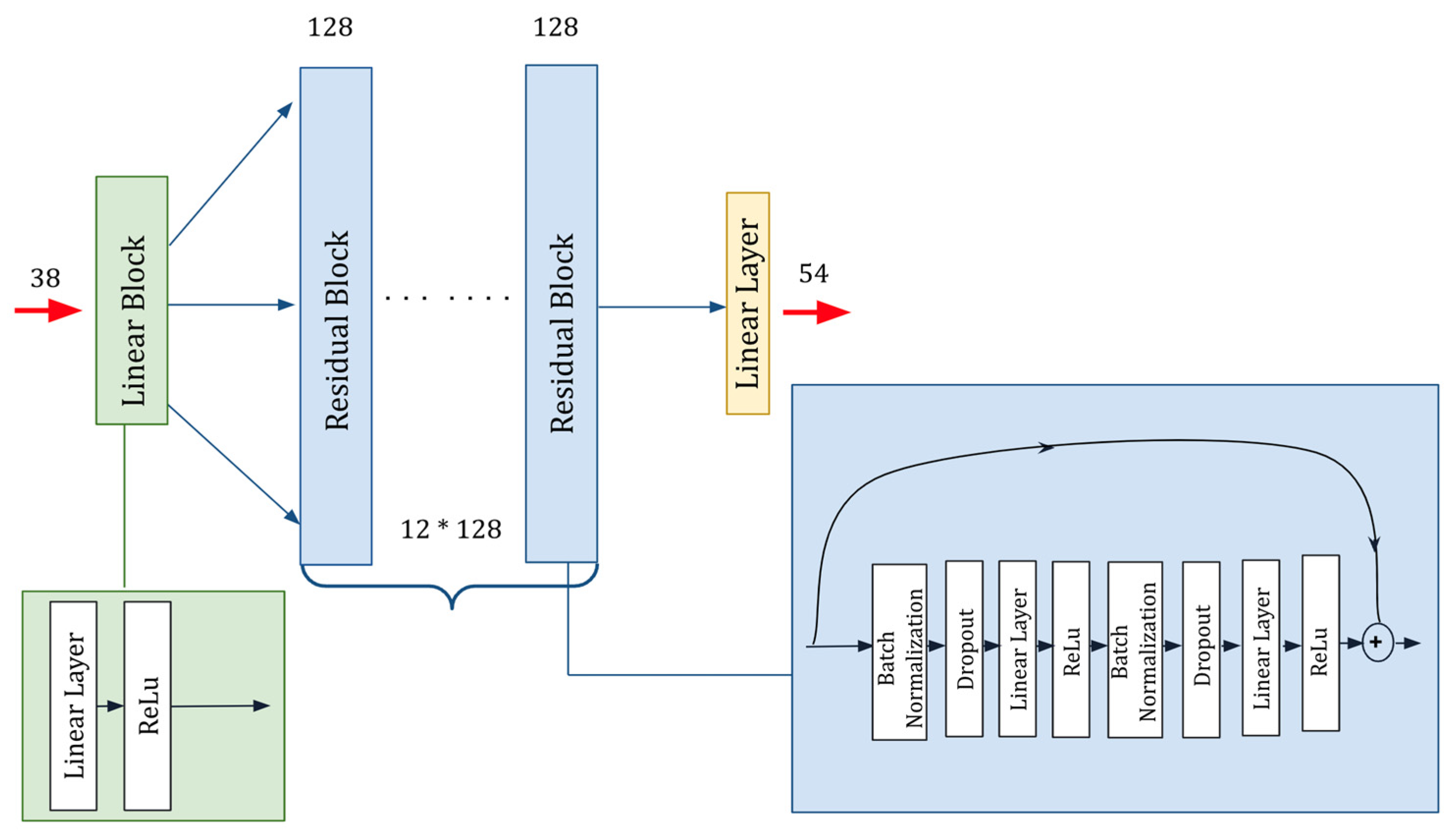
Figure 1. Schematic of the architecture of the model—dimension and structure of layers—the model has a linear block containing a linear layer and ReLu activation function followed by 12 residual blocks—each block containing two batch normalizations, two dropout layers, two ReLu activation function, and two linear layers and the last layer is a linear layer—dimension of input and output layers are 38 and 54, respectively which is the number of selected inputs and outputs of COPPER.
Energies 16 01352 g001
Figure 2. The selected regression plots—they show the relationship between the outputs of the proposed model and the actual values of the test data set. The x-axis represents the actual values of COPPER results, while the y-axis represents the predicted values of the surrogate model. The red line (x = y) corresponds to the highest level of accuracy, where the predicted and actual values are the same. The closer the blue dots are to the red line, the more accurate the predictions of the model are. (a,b) represent the lowest R-squared values among all 54 regression plots, (c,d) represent the average R-squared values, and (e,f) represent the highest R-squared values. These plots allow for visualization of the model’s performance and can be used to identify outputs where the model may not be performing as well.
Energies 16 01352 g002
Figure 3. This heat map shows the relationship between the inputs (x-axis) and outputs (y-axis) in 2030. It includes only design variables that have variations in the training dataset. The correlations are color-coded based on the shape of input-output correlation plots. The plots are scaled for each output based on the minimum and maximum values, so the relationships depicted in the heat map are relative to the specific output being considered. The heat map provides a visual representation of how each input affects each output and allows for easy identification of the strongest relationships.
Energies 16 01352 g003
Figure 4. This heat map shows the relationship between the inputs (x-axis) and outputs (y-axis) in 2040. It includes only design variables that have variations in the training dataset. The correlations are color-coded based on the shape of input-output correlation plots. The plots are scaled for each output based on the minimum and maximum values, so the relationships depicted in the heat map are relative to the specific output being considered. The heat map provides a visual representation of how each input affects each output and allows for easy identification of the strongest relationships.
Energies 16 01352 g004
Figure 5. This heat map shows the relationship between the inputs (x-axis) and outputs (y-axis) in 2050. It includes only design variables that have variations in the training dataset. The correlations are color-coded based on the shape of input-output correlation plots. The plots are scaled for each output based on the minimum and maximum values, so the relationships depicted in the heat map are relative to the specific output being considered. The heat map provides a visual representation of how each input affects each output and allows for easy identification of the strongest relationships.
Energies 16 01352 g005
Figure 6. National Gas and Wind Generation Capacity in 2030. Ranked factors affecting Canadian gas and wind generating capacities in 2030 are presented in bar charts. These are quantitative measures of the relative impact of system inputs on two key components of the Canadian energy supply mix, with the parameters listed on the y-axis. These values, which show correlation intensity, are normalized maximum derivatives of gas and wind capacities with respect to each input on the y-axis. The negative values show the negative correlations, positive values show positive correlations, and the absolute values of maximum derivatives represent the correlation intensity.
Energies 16 01352 g006
Figure 7. National Gas and Wind Generation Capacity in 2040. Ranked factors affecting Canadian gas and wind generating capacities in 2040 are presented in bar charts. These are quantitative measures of the relative impact of system inputs on two key components of the Canadian energy supply mix, with the parameters listed on the y-axis. These values, which show correlation intensity, are normalized maximum derivatives of gas and wind capacities with respect to each input on the y-axis. The negative values show the negative correlations, positive values show positive correlations, and the absolute values of maximum derivatives represent the correlation intensity.
Energies 16 01352 g007
Figure 8. National Gas and Wind Generation Capacity in 2050. Ranked factors affecting Canadian gas and wind generating capacities in 2050 are presented in bar charts. These are quantitative measures of the relative impact of system inputs on two key components of the Canadian energy supply mix, with the parameters listed on the y-axis. These values, which show correlation intensity, are normalized maximum derivatives of gas and wind capacities with respect to each input on the y-axis. The negative values show the negative correlations, positive values show positive correlations, and the absolute values of maximum derivatives represent the correlation intensity.
Energies 16 01352 g008
Table 1. Simulation dataset input range. The input values for running COPPER are randomly selected in each of these ranges.
Input VariableRangeUnit
Carbon tax50–750$/ton
Total demand growth 2050/20181.4–2.8Ratio
Annualized capital cost of natural gas106.687–130.396$/kW
Annualized capital cost of diesel159.148–194.514$/kW
Annualized capital cost of coal449.183–549.00$/kW
Annualized capital cost of nuclear795.514–972.295$/kW
Annualized capital of cost biomass (waste)465.161–568.531$/kW
Annualized capital cost of gas simple cycle (gasSC)83.478–102.029$/kW
Annualized capital cost of wind119.447–167.226$/kW
Annualized capital cost of solar85.602–142.670$/kW
Table 2. Model architecture experiment—a sample of higher accuracy architectures and associated prediction errors for training and test datasets.
ArchitectureTraining Error (MSE Loss)Test Error (MSE Loss)
1 linear + 12 Residual blocks, Neurons per block = 128, Dropout ratio = 0.5
Batch size = 128, Learning rate = 0.001
0.0100.049
1 linear + 13 Residual blocks, Neurons per block = 128, Dropout ratio = 0.5
Batch size = 128, Learning rate = 0.001
0.0180.06
9 linear blocks, Neurons per block = 128, Dropout ratio = 0.5
Batch size = 128, Learning rate = 0.001
0.0120.08
10 linear blocks, Neurons per block = 128, Dropout ratio = 0.5
Batch size = 128, Learning rate = 0.001
0.020.09
1 linear + 12 Residual blocks, Neurons per block = 128, Dropout ratio = 0
Batch size = 128, Learning rate = 0.001
0.050.1
1 linear + 12 Residual blocks, Neurons per block = 128, Dropout ratio = 0.5
Batch size = 128, Learning rate = 0.001
0.040.09
1 linear + 12 Residual blocks, Neurons per block = 512, Dropout ratio = 0.5
Batch size = 128, Learning rate = 0.0001
0.030.1
1 linear + 12 Residual blocks, Neurons per block = 512, Dropout ratio = 0.5
Batch size = 128, Learning rate = 0.01
0.060.09
Table 3. Selected model architecture with the highest accuracy.
Architecture
1 linear + 12 Residual blocks
Neurons per block = 128
Dropout ratio = 0.5
Batch size = 128
Learning rate = 0.001
25,000 steps (2000 epochs)
Table 4. Input-output relationship types and interpretations.
ShapeSample PlotInterpretation
NegativeEnergies 16 01352 i001The output will decrease with the selected input.
Strongly negativeEnergies 16 01352 i002The output will rapidly decrease with the selected input.
Relatively insensitiveEnergies 16 01352 i003The output’s variation with respect to the input is not significant relative to its variation with respect to other inputs. Note that these values are normalized, so this does not necessarily imply there is a constant relationship.
PositiveEnergies 16 01352 i004The output will increase with the selected input.
Strongly positiveEnergies 16 01352 i005The output will rapidly increase with the selected input.
Inconclusive (unknown)Energies 16 01352 i006There is no identifiable pattern in the correlation between the input and the output.
Bell-shapedEnergies 16 01352 i007The output increases, peaks, and then decreases with respect to the input.
Inverse bell-shapedEnergies 16 01352 i008The output decreases, reaches a trough, and then increases with respect to the input.
Table 5. Performance of the proposed model in terms of MSE losses and R-squared distribution for the test data set.
Training LossValidation LossTest LossMean R-SquaredR-Squared Standard Deviation
0.010.0470.0490.930.05
Table 6. Comparison of COPPER and proposed model computational costs and run time.
ModelCPUMemoryRun-Time
COPPER16–3264–128 GB11 h–72 h
Residual neural network1NA *17.1 ms
* Except for saving the model and associated data.
Disclaimer/Publisher’s Note: The statements, opinions and data contained in all publications are solely those of the individual author(s) and contributor(s) and not of MDPI and/or the editor(s). MDPI and/or the editor(s) disclaim responsibility for any injury to people or property resulting from any ideas, methods, instructions or products referred to in the content.