Measuring and Modeling the Skin Effect for Harmonic Power Flow Studies

Abstract

This research aims to quantify the skin effect and estimate expressions that well represent the phenomenon for harmonic power flow studies. The primary focus is to validate the behavior of the skin effect at harmonic frequencies ranging from 60 Hz to 960 Hz, while considering various amplitudes of electric current. The investigation not only examines the measurement of the skin effect, but also considers the temperature of the tested conductors, aiming to analyze the increase in resistance resulting from temperature rise and resistivity changes. The measurement outcomes demonstrate notable increments in electrical resistance, with resistivity increases of up to 1.9% observed throughout the measurement process. Finally, based on the results obtained through laboratory measurements, mathematical expressions were estimated as a function of frequency. In order to evaluate the simulation time reduction by the proposed expressions, OpenDSS (version: 9.4.1.2; Electric Power Research Institute, Knoxville, TN, USA) software was used, which aims at quantifying the impact of the skin effect on the technical losses. The results from these simulations demonstrate that the proposed expressions to account for the skin effect in conductors reduce the simulation time by around 17% for harmonic power flow.

1. Introduction

The current harmonic and interharmonic components, which encompass an inseparable reality of electrical systems, have long been studied and quantified by researchers and engineers around the world. The presence of these components, particularly those operating at higher frequencies, on any electric circuit, causes an increase in the resistance of conductors due to the skin effect phenomenon.

Subsequently, scientific publications focused on investigating the skin effect by conducting measurements to establish a relationship between the resistance of the conductor at direct current (RDC) and the resistance of the conductor at alternating current (RAC), considering variations in frequency, such as [1]. Scientific literature that mathematically covers the phenomenon [2,3] was consolidated by utilizing Bessel’s equation as a faithful representation of the skin effect, where the particular behavior of the magnetic field for different conductors was later clarified, such as in hard wires and flexible cables [4].

Furthermore, laboratory experiments have addressed specific issues related to the measurement of electrical resistance in conductors at different frequencies [5]. These experiments involved the development of an electrical configuration capable of quantifying resistance under varying electric currents. In parallel, computer simulations have become essential tools for scientific advancements [6]. The use of finite element-based simulated meshes has enabled detailed analyses of the electromagnetic performance of various conductors and electrical equipment geometries.

Building upon previous research, recent scientific studies have focused on practical applications of the phenomenon, such as power losses in arc furnace buses [6]. Additionally, the scientific community has extensively examined the reliability of mathematical solutions provided by computer simulations [7].

However, a shared characteristic observed in the various studies conducted [6,7,8,9] is the lack of measurements and real-world applicability of the data to analyze the impact of the skin effect on electric power systems. This knowledge gap highlights the need for a better understanding of quantifying the skin effect. In line with this observation, the study conducted in [10] focused on the practical implications of the skin effect on electrical equipment, such as transformers, resulting in increased power losses.

Similarly, the study in [11] examined the behavior of the skin effect in a 69 kV conventional transmission line with ground return, offering practical insights into the phenomenon, albeit without fully considering the complex nature of the entire electrical system. Despite the innovative mathematical modeling presented, the study primarily addresses the individual impact of the skin effect on the specific electrical device, neglecting the comprehensive analysis of electrical power distribution systems as a whole.

While previous studies have explored the behavior of the skin effect in transformers and transmission lines, there are studies, such as [12,13], that leverage this phenomenon to develop a control logic for protecting a railway system with direct current rails. Specifically, this study presents a precise methodology for analyzing the skin effect in the time domain, accurately reproducing fault currents in the rails. In contrast to earlier research, this study satisfactorily considers the intricate complexities of the local power distribution system. In addition to the mentioned papers, [14] also addresses the phenomenon, pointing out that eddy currents and the skin effect play an important role in electrical machines and power systems.

The impact of harmonic components on eddy current losses in the core of soft magnetic materials is discussed in [13]. The study involves the creation of a 3D model based on the magnetic behavior of the material. Furthermore, the quantification of losses resulting from the skin effect induced by harmonic components was carried out. Ref. [15] presents an approach for analyzing the skin effect in a wire using finite elements. Although this study makes significant contributions to calculating conductor resistance as a function of frequency, it lacks laboratory exploration and measurement, which is an aspect addressed in the current study. Ref. [16] presents a singular contribution on cables losses via a computational method based on a probabilistic approach that predicts some features on litz cables. Despite the singular contribution that this study makes to quantifying losses on conductors, it lacks a focus on electrical power system conductors that the current study aims to fulfill.

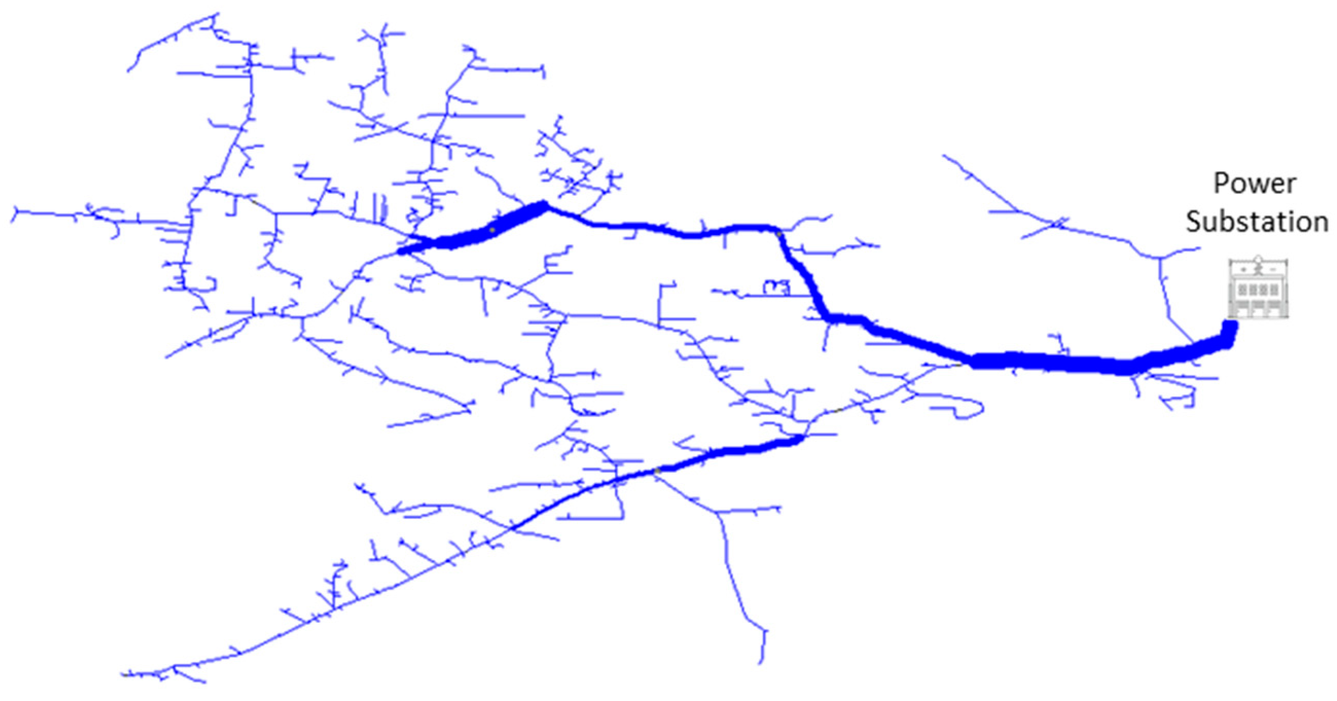
The study presented herein has as its objective to present the quantification of resistance increase due to the skin effect in conductors used on power distribution networks. To undertake this study, it is crucial to have a comprehensive understanding of the physical and mathematical aspects of the problem, as well as to conduct laboratory measurements. This allows for the quantification of the skin effect in the electrical resistance of various types of conductors in power distribution lines. Additionally, the expressions estimated for representing the skin effect in conductors were applied to the IEEE 8500-node test feeder utilizing the OpenDSS software, which assesses the impact that the suggested approach has in simulation time and the influence of the skin effect on power distribution losses. It is important to point out that not only are the results from these simulations displayed on item 4.2, but also a detailed approach regarding the electrical characteristics of IEEE 8500-node test feeder. The subsequent section will delve into the physical and mathematical aspects related to the phenomenon.

2. Theoretical Background

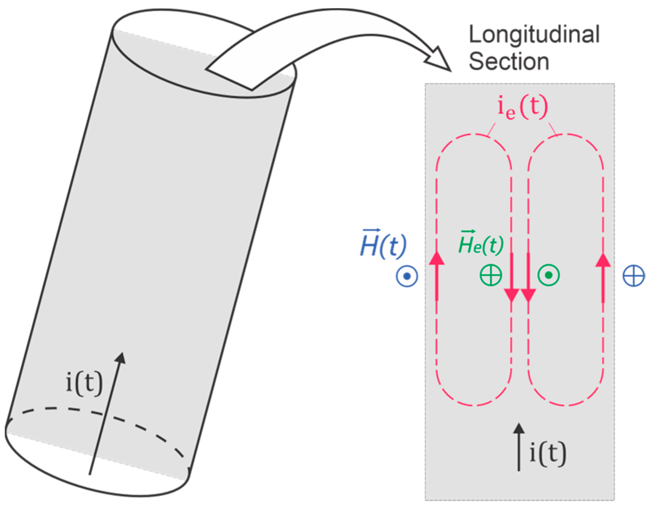
In essence, the skin effect consists of the non-uniformity of the electric current density in the cross-section of an electrical conductor. In other words, circular conductors, commonly used in power distribution systems, present a greater flow of electric current on the surfaces of the conductor than on its inner part, and this effect is amplified with increases in electrical current. This phenomenon occurs when a current $i\left(t\right)$ varying in time runs through the conductor and, as a result, a magnetic field $\overrightarrow{H}\left(t\right)$ is generated around it according to Ampere’s law. However, in accordance with the law of electromagnetic induction, any time-varying magnetic field generates an internal electromotive force (EMF) in the conductor that is also time-varying, but in the opposite direction to the $\overrightarrow{H}\left(t\right)$ from which it arises.

As such, a circulating current $i_e\left(t\right)$ arises due to the potential difference that is created between the innermost part of the conductor and its surface; as such, $\overrightarrow{H_e}\left(t\right)$ is generated by virtue of Ampère’s law. Figure 1 illustrates the previously mentioned electrical magnitudes. Additionally, Figure 1 displays a solid conductor exclusively for simplicity and clarity of the physical conceptualization of the before mentioned phenomenon. All of the conductors discussed throughout this paper are stranded conductors.

The law of electromagnetic induction guarantees energy conservation in the flow of electric charge within a conductor. It ensures that, despite the presence of a time-varying magnetic field surrounding the conductor, the resulting electric current remains continuous and does not alter the quantity of charges passing through the conductor’s cross-sectional area. On the other hand, it modifies the current density along this cross-section, thus distinguishing the physical process that characterizes the skin effect [17]. The currents that arise inside the conductor $i_e\left(t\right)$ are denominated as eddy currents, as shown in Figure 1. In the skin effect, the electric current density of the conductor is not uniform. The inner part the resulting current intensity is $i\left(t\right)-i_e\left(t\right)$, while closer to the surface, the current is $i\left(t\right)+i_e\left(t\right)$, and this is the main cause of the non-uniform distribution of the current density in its cross-section.

Mathematical Approach

To mathematically contemplate the skin effect, it is necessary to address the behavior of the magnetic field generated by the electric current that runs through the conductor. In this sense, the magnetic field is time-varying and can be expressed by (1), just as the electric field can be represented by (2).

$$\overrightarrow{H}\left(z,t\right)=H_y\left(z\right)Re\left[e^{j\omega t}\right]\overrightarrow{a_y}$$

(1)

$$\overrightarrow{E}\left(z,t\right)=E_x\left(z\right)Re\left[e^{j\omega t}\right]\overrightarrow{a_x}$$

(2)

Therefore, by applying (1) and (2) to Ampere’s law and the law of electromagnetic induction, respectively, while considering that the electric field also varies in time and is perpendicular to the direction of $\overrightarrow{H}\left(z,t\right)$, one arrives at (3) and (4).

$$\nabla \times \overrightarrow{E}=\frac{\partial E_x\left(z\right)}{\partial z}\overrightarrow{a_y}=-j\omega \mu H_y\left(z\right)\overrightarrow{a_y}$$

(3)

$$\nabla \times \overrightarrow{H}=-\frac{\partial H_y}{\partial z}\overrightarrow{a_x}=j\omega \epsilon E_x\left(z\right)\overrightarrow{a_x}$$

(4)

Under the intent of obtaining a differential equation that relates only to the magnetic field, expression (4) is rotated.

$$\nabla \times \left(\nabla \times \overrightarrow{H}\right)=j\omega \epsilon \nabla \times \left(E_x\left(z\right)\overrightarrow{a_x}\right)$$

(5)

Substituting the Laplacian vector Equation (6) into (5), one arrives at (7).

$${\nabla }^2\overrightarrow{H}=\nabla \left(\nabla ·\overrightarrow{H}\right)-\nabla \times \left(\nabla \times \overrightarrow{H}\right)$$

(6)

$$\nabla \left(\nabla ·\overrightarrow{H}\right)-{\nabla }^2\overrightarrow{H}=j\omega \epsilon \nabla \times \overrightarrow{E}$$

(7)

As $\overrightarrow{H}\left(z,t\right)$ is a vector field that has a zero divergence, it is possible to rewrite (7) according to Gauss’ law, considering the calculation of the magnetic field gradient, and replacing (3) in (7); one arrives at (8).

$$\frac{{\partial }^2{H}_y\left(z\right)}{{\partial z}^2}=-{\omega }^2\mu \epsilon H_y\left(z\right)$$

(8)

Since expression (8) is the Helmholtz equation in phasor form [18], one can specify the Helmholtz equation as (9) and define the propagation constant of the magnetic field (10) utilizing a conductive material.

$$\frac{\frac{{\partial }^2{H}_y\left(z\right)}{{\partial z}^2}}{H_y\left(z\right)}=-{\lambda }^2=-{\omega }^2\mu \epsilon$$

(9)

$$\lambda =\omega \sqrt{\mu \epsilon }=\omega \sqrt{\mu \epsilon \prime \left(1-j\frac{\sigma }{\omega \epsilon \prime }\right)}$$

(10)

Noteworthy is that for conducting materials $\frac{\sigma }{\omega \epsilon \prime }\gg 1$ as such, (10) is summarized as the following:

$$\lambda =\left(1+j\right)\sqrt{\pi f\mu \sigma }=\alpha +j\beta$$

(11)

In this sense, the solution to the Helmholtz equation presents the behavior of the magnetic field. It enhances the context to clarify the physical significance of the propagation constant for the skin effect. The solution to the Helmholtz equation is given by the following:

$$\overrightarrow{H}\left(z,t\right)=H_0{e}^{-\alpha }{e}^{j\left(\omega t-\beta z\right)}\overrightarrow{a_y}$$

(12)

In (12), the term $e^{j\left(\omega t-\sqrt{\pi f\mu \sigma }z\right)}$ represents the oscillatory feature of the magnetic field, where $\beta$ proposes the phase shift. However, the term $e^{-\sqrt{\pi f\mu \sigma }z}$ presents exponential decay $\alpha$ of the original magnitude of the vector field ($H_0$) as the wave travels in the direction +z. Through these equations, it is possible to define the skin effect by means of skin depth. The skin depth $\delta$ corresponds to the distance traveled by the magnetic field in the material medium in which its original magnitude is decreased in the order of $e^{-1}$. In other words, skin depth elucidates the degree of penetration of the magnetic field and of the circulating internal currents in a conductor with losses [18], as shown in Figure 2. Therefore, for the condition presented in (12), z should be equal to $1/\sqrt{\pi f\mu \sigma }$ for attenuation on the order of $e^{-1}$, where the skin depth is defined as the following:

$$\delta =\frac{1}{\sqrt{\pi f\mu \sigma }}$$

(13)

Hence, the skin effect can be mathematically defined as the skin depth in a conductor, as represented by (13), and it physically signifies a higher concentration of current in the cross-section of the conductor, as depicted in Figure 2. Therefore, it is crucial to investigate how the current density varies based on the conductor’s geometry. With this in mind, significant emphasis is placed on studying the current distribution of various types of conductors. As a result, in (14), two different forms are used to calculate the current through a conductor, such as the surface integral of $J$ and Ampère’s law.

$$Hr=\underset{0}{\overset{r}{\int }}Jrdr$$

(14)

To understand how the geometry of the conductor influences the current density of the conductor, one derives (14) concerning the radius of the conductor. Furthermore, it is also pertinent to derive (14) in time, since the magnetic field is a function of this variable, resulting in the following:

$$\frac{dJ}{dt}=\frac{d^{2}H}{drdt}+\frac{1}{r}\frac{dH}{dt}.$$

(15)

The result of (15) provides the variation of the current density in the conductor for these two variables, space (r) and time (t), according to the variations of the magnetic field. In this way, the following developments will be directed to finding mathematical expressions for the derivatives of the magnetic field in time and space in simpler forms for the result of (15). Noteworthy still is that $\overrightarrow{E}=\rho \overrightarrow{J}$, thus $\mu dr\frac{dH}{dt}=\rho \overrightarrow{J}$, where one arrives at (16) and substitutes (16) into (15), one obtains (17), which is the differential equation that models the phenomenon presented in Figure 2, in a way that specifies the density of the electric current along the cross-section of the conductor.

$$\frac{dH}{dt}=\frac{\rho }{\mu }\frac{d\overrightarrow{J}}{dr}$$

(16)

$$\frac{d^{2}J}{d{r}^2}+\frac{1}{r}\frac{dJ}{dr}-\frac{\mu }{\rho }\frac{dJ}{dt}=0$$

(17)

Moreover, in the phasor form, where d/dt $\to$ j$\omega$ and $k^2=j\omega \mu \sigma$, one has the following:

$$r^2\frac{d^{2}J}{d{r}^2}+r\frac{dJ}{dr}-r^2{k}^{2}J=0.$$

(18)

The differential equation shown in (18) has the term r²k² arranged to facilitate the mathematical development to reach an elegant solution. The expression (19) is the electric current density as a function of the radius of the conductor under analysis, expressed by Bessel’s equations with 0 and 1 indexes (I₀ and I₁) [18,19]. The differential equation shown in (18) is a function of r₀, which is the conductor radius, and r represent the variable, which determines the intensity of the electric current in the cross-section of the conductor, as shown in (19). It is important to note that on (18) the term r²k², during the mathematical development to reach a solution, turns into kr within the Bessel’s expressions of indexes 0 and 1.

$$J\left(r\right)=\frac{Ik}{2\pi r_0}\frac{I_0\left(kr\right)}{I_1\left(k{r}_0\right)}$$

(19)

Considering that the current density, when a direct current runs through the conductor is $J_{DC}=I/\pi r_0^2$, then $J\left(r\right)/J_{DC}$ is given by the following:

$$\frac{J\left(r\right)}{J_{DC}}=\frac{\left(\left(1+j\right)\left(\frac{r_0}{\delta }\right)\right)}{2}\frac{I_0\left(\left(1+j\right)\left(\frac{r_0}{\delta }\right)\left(\frac{r}{r_0}\right)\right)}{I_1\left(\left(1+j\right)\left(\frac{r_0}{\delta }\right)\right)}$$

(20)

Notably, the current density on the outer part of the conductor is greater in conductors with larger cross-sections, thus underscoring the impact of the skin effect [18,19]; this is evident from (20) as well. Therefore, the electrical resistance of conductors under such conditions increases, which implies an increase in power losses due to the transport of active power. Consequently, to evaluate the impact of such a phenomenon, the proposal is put forward for the study of the behavior of $\raisebox{1ex}{$R_{AC}$}\!\left/ \!\raisebox{-1ex}{$R_{DC}$}\right.$, in similar fashion to the approach already used for current density $\left(\raisebox{1ex}{$J_{AC}$}\!\left/ \!\raisebox{-1ex}{$J_{DC}$}\right.\right)$.

When considering the resistance in alternating current $\left(R_{AC}\right)$, one uses Ohm’s law, as seen in (21), with the ratio being $\raisebox{1ex}{$R_{AC}$}\!\left/ \!\raisebox{-1ex}{$R_{DC}$}\right.$ as presented in (22) [19,20].

$$Z=\frac{\rho l}{\pi r_0}\frac{k}{2}\frac{I_0\left(k{r}_0\right)}{I_1\left(k{r}_0\right)}$$

(21)

$$\frac{R_{AC}}{R_{DC}}=Re\left\{\frac{J\left(r_0\right)}{J_{DC}}\right\}$$

(22)

It is observed in (22) that as the ratio $\frac{r_0}{\delta }$ increases, the electrical resistance of the conductor increases proportionally for a conductor with radius $r_0$ and with a skin depth that decreases (increasing the ratio $\frac{r_0}{\delta }$). A trivial condition concerning the increase in ratio $\frac{r_0}{\delta }$ occurs when harmonic components of electric current flow through the conductor. Under such conditions, harmonic components imply a decrease in the value of $\delta$, in accordance with (13). Indirectly, this causes an increase in the resistance of the conductor, as it increases the ratio $\frac{r_0}{\delta }$ [18,21].

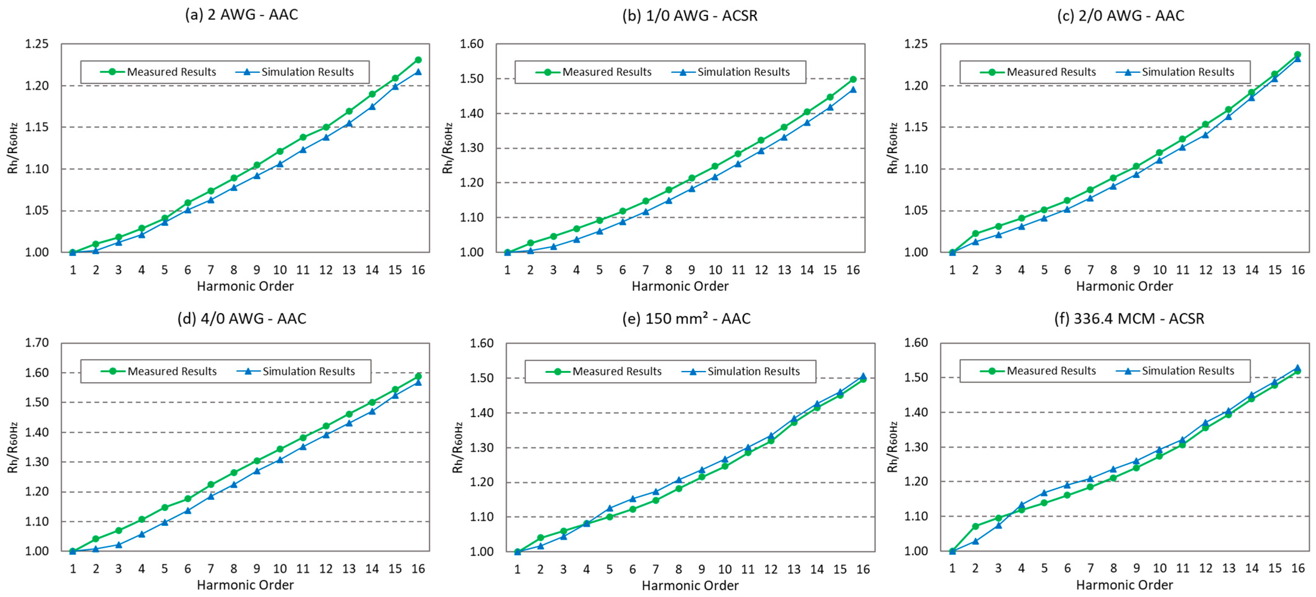
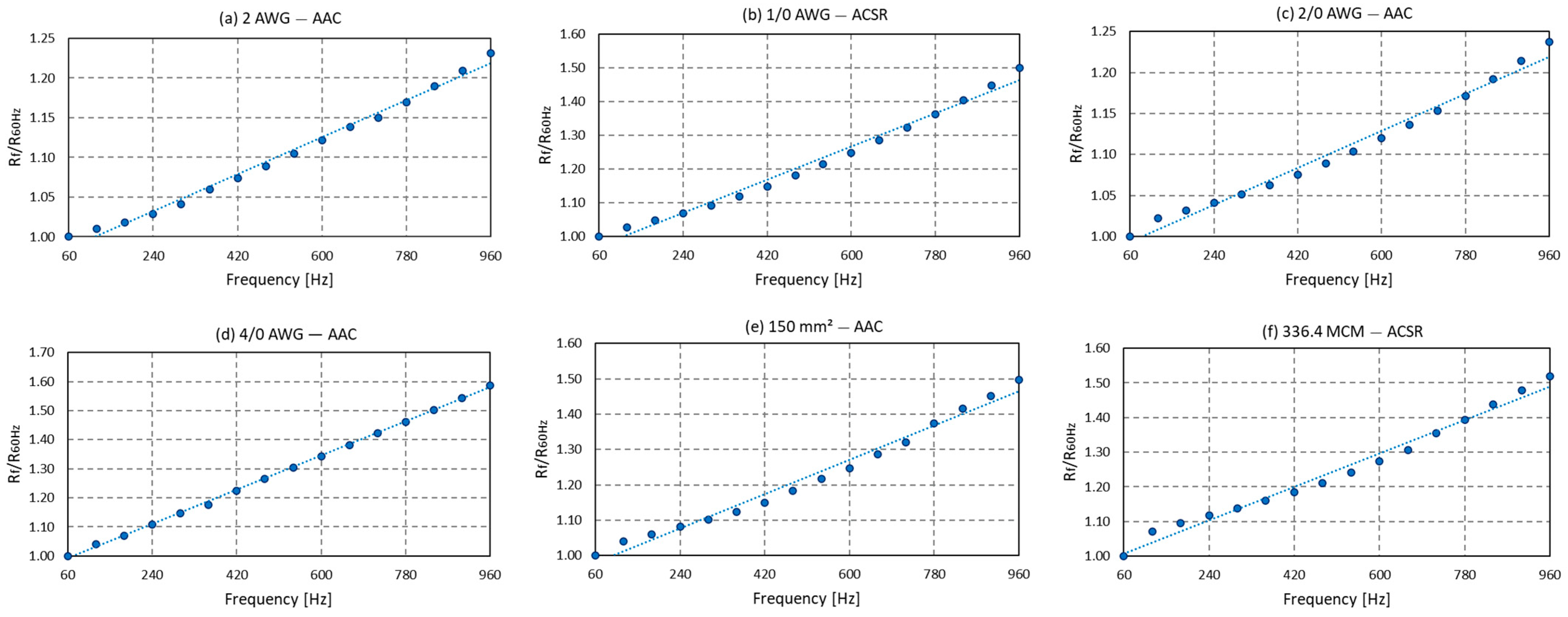
It is well established that harmonic components are inherent in electrical power systems, particularly in power distribution systems. In such systems, it is common to encounter harmonic currents (and correspondingly, voltages) with frequencies up to 960 Hz (16th harmonic order). Beyond this frequency range, the amplitudes of these components become insignificant, exerting minimal impact on the skin effect.

In the specific case of electrical power distribution systems, the skin effect assumes a very applicable role in harmonic power flow studies, especially on medium- and low-voltage power networks. In this sense, the physical–mathematical development carried out so far aimed at establishing physical foundations for understanding the phenomenon, concerning justifying any sensible increase in resistance of the conductor under non-sinusoidal conditions, as well as justifying the investigation into the quantification of this increase. From this standpoint, the objective of this study is to assess the electrical resistance of various conductors employed in power distribution systems, in order to quantify the rise in resistance attributed to the aforementioned phenomenon. The subsequent section outlines the methodology employed to measure the electrical resistance of conductors affected by the skin effect.

3. Measurement Methodology

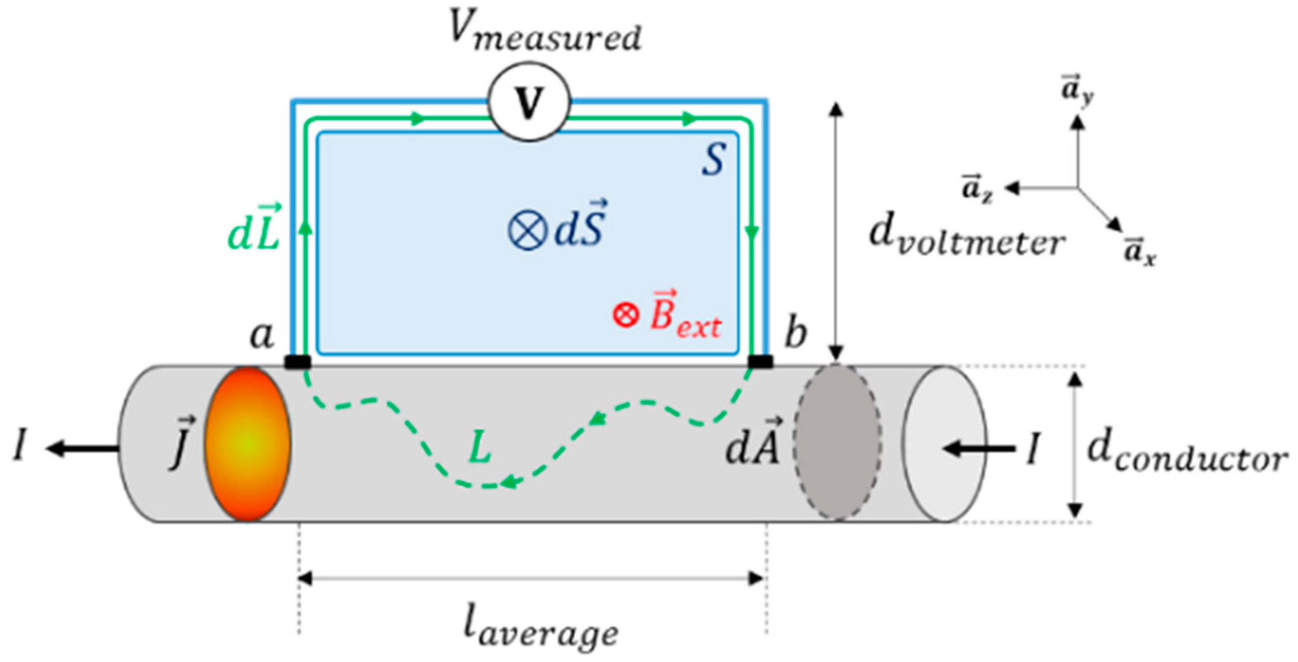
In pursuance of measuring the impact of the skin effect on conductors, it is necessary to understand which electrical magnitudes are verified in the measurement methodology. Given the relatively low magnitude of the measured quantities, it is crucial to consider the uncertainties associated with the measurements. To determine the resistance of the conductor, an indirect measurement approach was employed. This involved passing an electric current through the conductor under examination and using an oscilloscope to measure the corresponding voltage drop. By applying Ohm’s Law, the resistance of the conductor can be calculated using Equation (23).

$$R=\frac{1}{l_{average}}Re\left\{\frac{{\dot{V}}_{measured}}{\dot{I}}\right\}\times 1000\left[\frac{\mathsf{\Omega }}{\mathrm{km}}\right]$$

(23)

However, to obtain a reliable measurement of the voltage drop in the conductor, an assessment is made into the possible interferences admitted by the voltage loop. That said, voltmeters, when measuring the potential difference between two points a and b, are known to consider the voltage arising from the conservative electric field between these two points. This is in addition to the voltage from the non-conservative magnetic field that varies in time and passes through the loop voltage, where (24) is the potential difference measured by the oscilloscope, which includes both previously mentioned vector fields.

$$V_{measured}\approx \underset{a}{\overset{b}{\int }}\overrightarrow{E}·d\overrightarrow{L}+\frac{\partial }{\partial t}\underset{0}{\overset{d}{\int }}\underset{a}{\overset{b}{\int }}{\overrightarrow{B}}_{ext}·d\overrightarrow{S}$$

$$V_{measured}\approx \underset{a}{\overset{b}{\int }}Edz+\frac{\partial }{\partial t}\underset{0}{\overset{d}{\int }}\underset{a}{\overset{b}{\int }}Bdzdy$$

(24)

In this context, the measurement methodology used assumes two origins for the potential difference ascertained in the oscilloscope. The first comes from $\overrightarrow{E}$ that is independent of the integration path inside the conductor, as well as from the voltage induced by the variation of ${\overrightarrow{B}}_{ext}$ in time bound to the voltage loop, as shown in Figure 2. Additionally, Figure 2 displays a solid conductor exclusively for simplicity and clarity of the physical conceptualization of the before mentioned measurement methodology. All of the conductors measured in this study are stranded conductors.

From Figure 2, it can be noted that ${\overrightarrow{B}}_{ext}$ passes through the voltage loop S, where an induced voltage appears between the conductor points a and b, which is measured with the oscilloscope, and constitutes an effective value of the voltage $V_{measured}$, as shown in (24). It is important to point out that the induced voltage in question greatly impacts the measurement, due to the low order of magnitude of the voltage arising from $\underset{a}{\overset{b}{\int }}\overrightarrow{E}·d\overrightarrow{L}$between points a and b. In this case, the smallest possible voltage loop is used to minimize the impact of the voltage induced by ${\overrightarrow{B}}_{ext}$. In accordance with [16], the suggestion is that the height of the voltage loop equals the conductor diameter. More objectively, $d_{voltmeter}=d_{conductor}$ while considering the setup in Figure 2.

In addition to taking electromagnetic factors into account when measuring the electrical resistance of conductors, it is important to consider the presence of nearby conductive materials. These materials can induce eddy currents through the proximity effect, potentially interfering with the measurement procedure. To mitigate this issue, all conductive materials were positioned at a distance of more than one meter from the measurement setup [22,23].

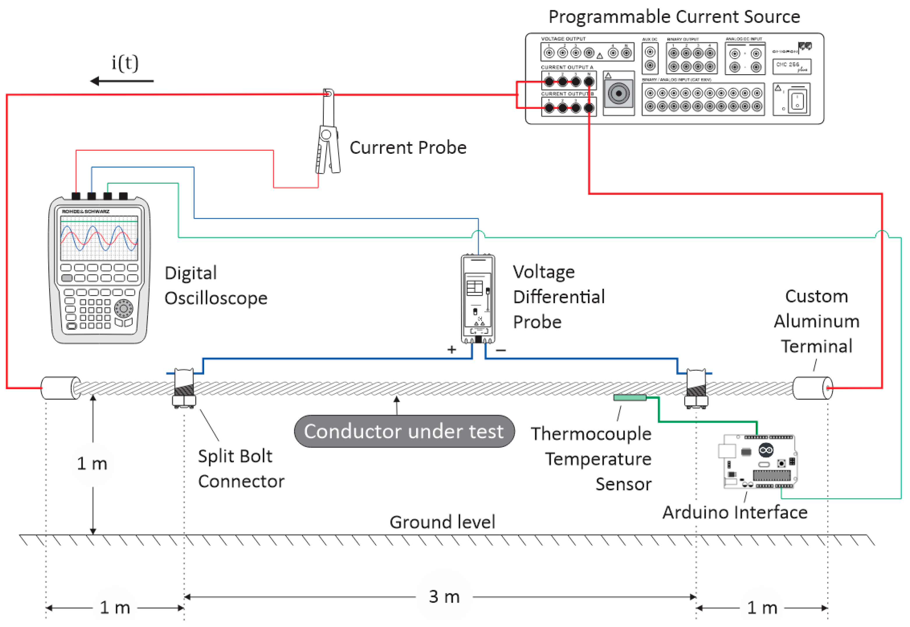
In this manner, Figure 3 illustrates the measurement setup used to measure the resistance of the conductors. Figure 3 shows the programmable source, CMC 256 plus, manufactured by Omicron Electronics Corp. (Houston, TX, USA), used to operate as a current source. In addition, there is a digital oscilloscope, RTH1004, manufactured by Rohde & Schwarz (Teisnach, Germany), with four isolated channels and a 5 GSa/s sampling rate.

In order to fully describe the measurement setup, the main characteristics are stated as follows:

• The ground is composed of concrete.
• The current return path is 1 m from the conductor under test, close to ground level.
• Wooden racks were used as a non-conductive material to keep the conductor under testing 1 m away from ground level.
• Voltage differential probes cables were placed according to $d_{voltmeter}=d_{conductor}$ for each conductor, as displayed in Figure 2 and Figure 3.

The sensors used for the acquisition of electrical quantities were the A622, manufactured by Tektronix (Portland, OR, USA), employed for the acquisition of electric current, and the TA041, manufactured by PicoTech (Cambridge, UK), for the acquisition of the voltage signal. The configuration displayed in Figure 3 shows the electronic devices used, as well as the three crucial items for reaching the objective of this study.

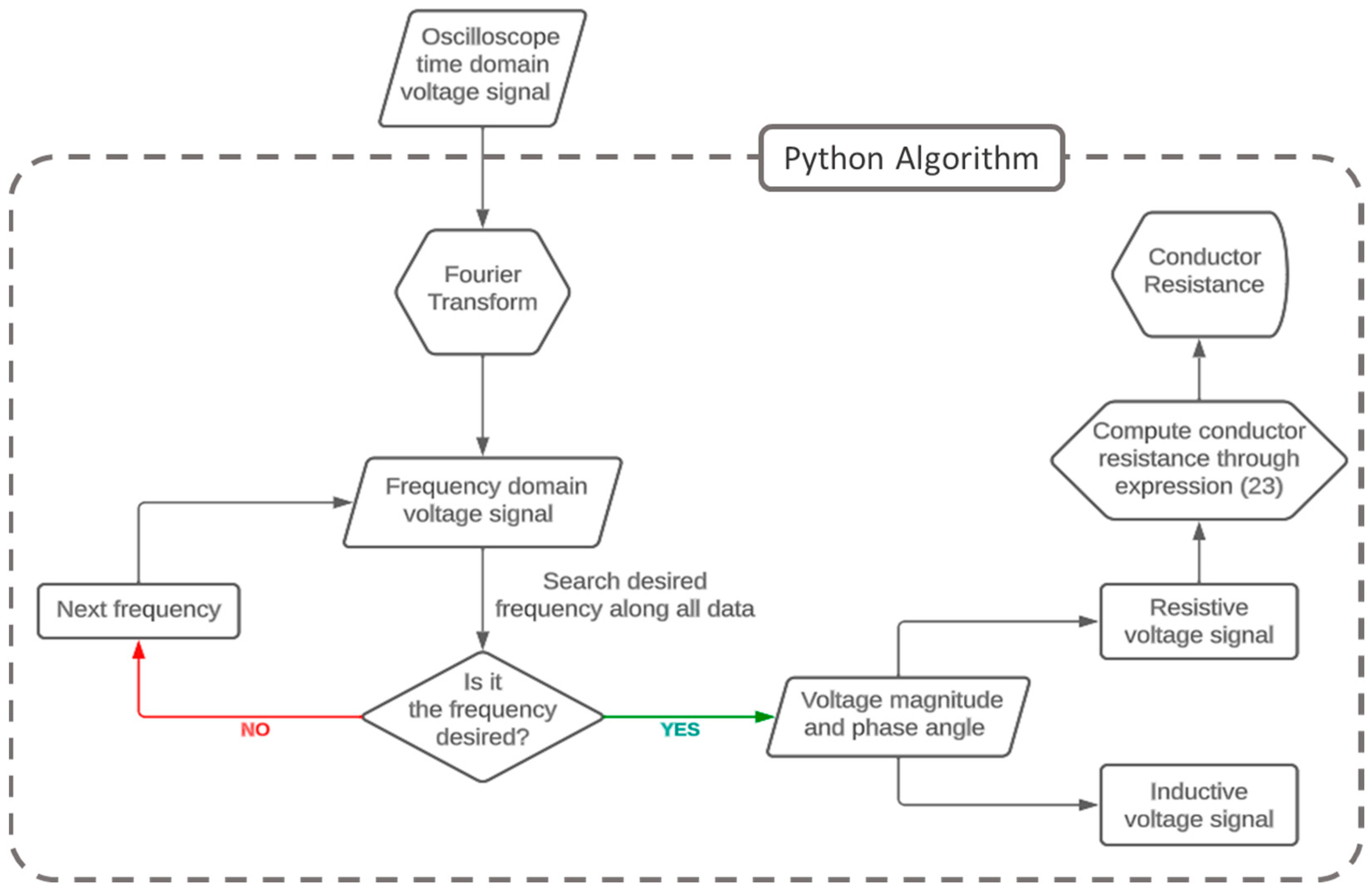
Additionally, the post-processing voltage signal registered on the oscilloscope corresponds to the flow chart presented in Figure 4. Briefly, the oscilloscope registered a time domain signal that was applied to a Python algorithm developed exclusively to perform Fourier transforms. Its purpose is to obtain the voltage magnitude and phase angle of the desired frequency, which is the current frequency flowing through the conductor under test. It is important to highlight that the reference phase angle (0° electrical degrees) is related to the current signal, once the programmable power source is a current source. Additionally, the magnitude of the out-of-phase inductive voltage signal is larger than the resistive voltage signal, especially regarding high frequencies. It is an expected response, since the inductive part of the conductor responds to a linear relation to frequency; meanwhile, the resistive part responds according to (22) in relation to frequency. In other words, the measured voltage signals presented a phase angle higher than 80°, indicating that voltage is predominantly inductive. The considered resistive voltage signal was computed (see Figure 4) and applied to (23), obtaining the conductor’s electrical resistance.

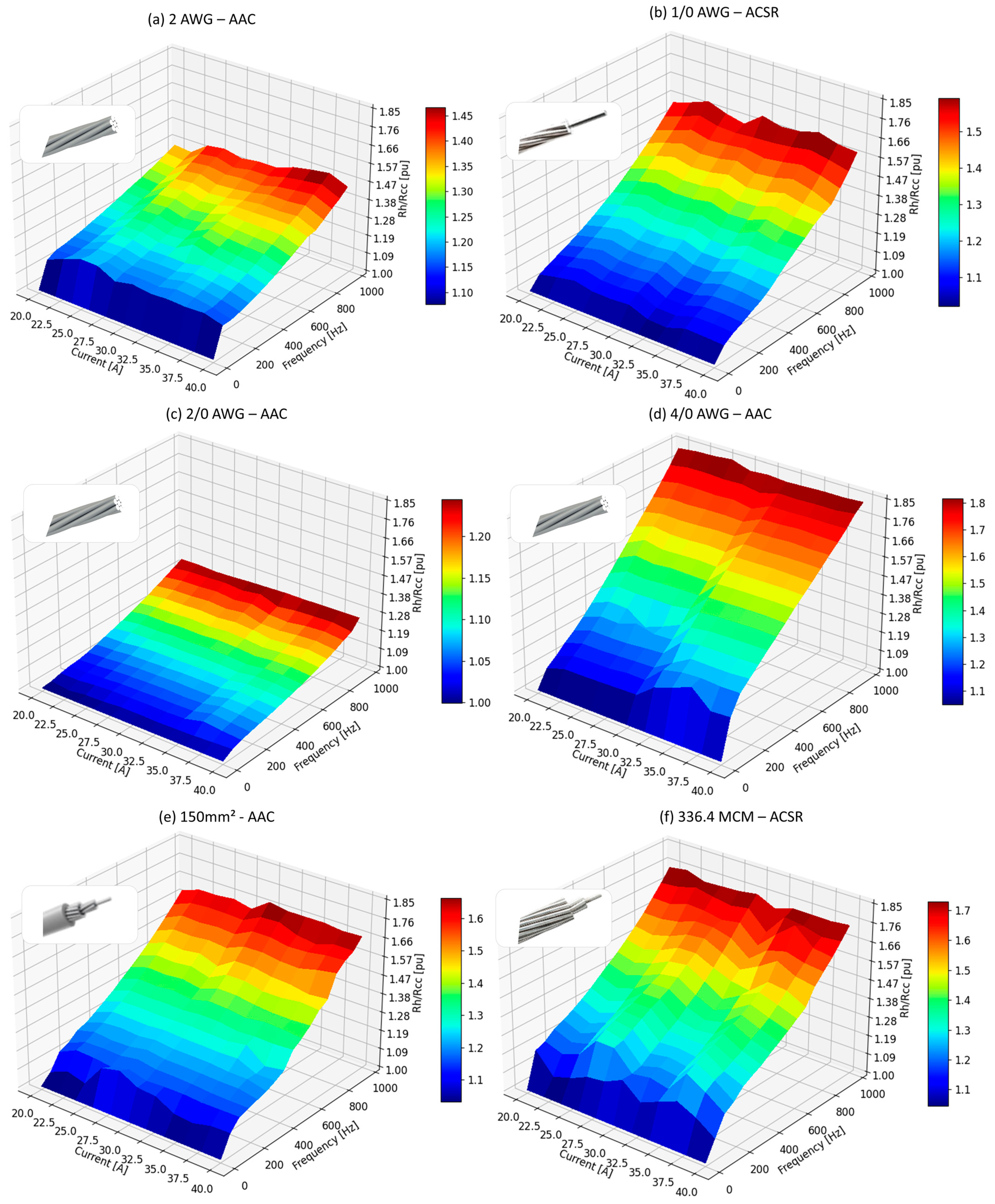
Firstly, the conductor under test in this study includes the main conductors used in electrical power distribution systems, which are 2 AWG—AAC, 1/0 AWG—ACSR, 2/0 AWG—AAC, 4/0 AWG—AAC, 150 mm² protected and 336.4 MCM—ACSR. Here, it is noteworthy that for better contact between the power source conductors (red thicker lines, Figure 3) and the conductor under test, it is necessary to use terminals both for current injection in the conductor under test, as well as for measuring the voltage.

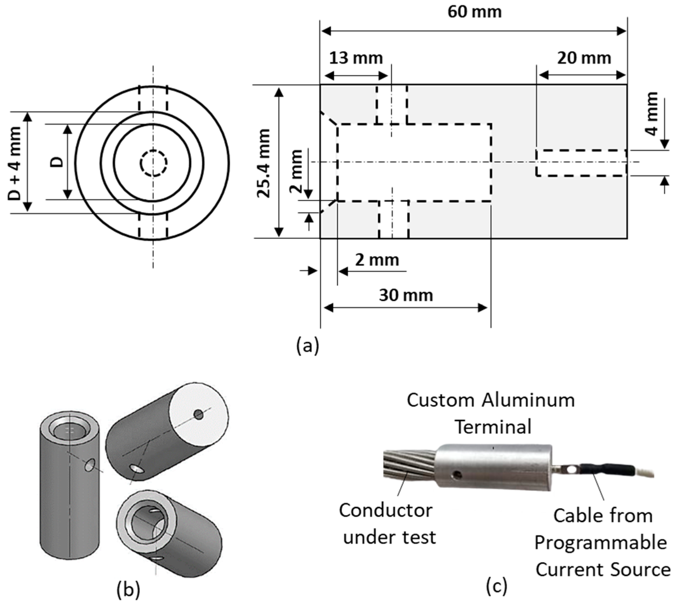
As shown in Figure 3, the aluminum terminal ensures that the electrical current is distributed as expected. To this end, its geometric dimensions are shown in Figure 5, where D represents the diameter of the conductor under test.

To ensure that the current distribution is homogeneous in the region where the voltage in the conductor is measured, a distance of 1 m from the input to the output terminals of the electric current was assumed. This implies that $\overrightarrow{J}$ is homogeneous in the cross-section of the conductor, guaranteeing an adequate measurement [23].

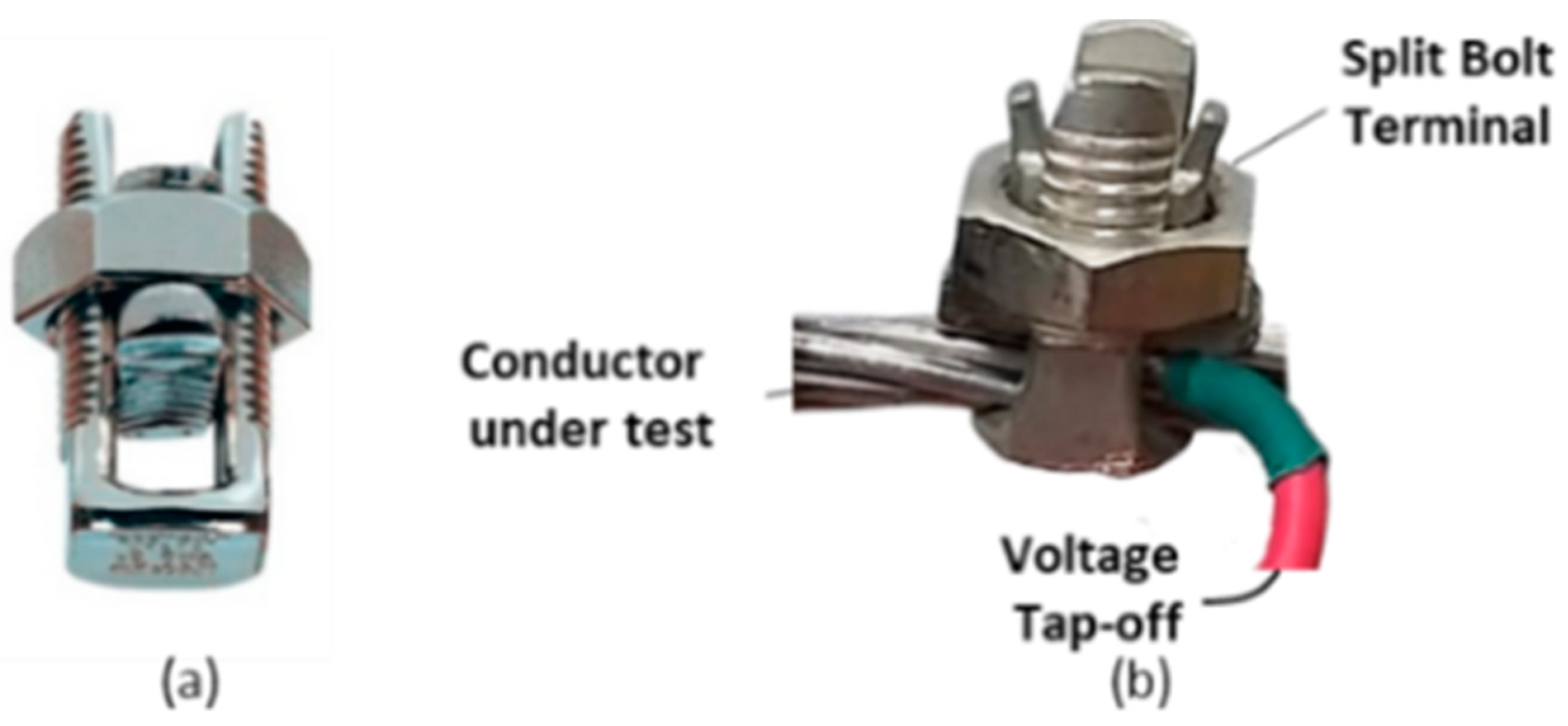
Finally, there are split bolt terminals for connecting the oscilloscope voltage channels, allowing for a better connection, as shown in Figure 6.

In addition to the previous recommendation regarding the voltage loop during the measurement of conductor electrical resistance, reference [23] also mentions the potential influence of temperature on the accurate quantification of resistances considering the skin effect.

This aspect is of great importance, since the electric current heats up the conductor and, consequently, increases the resistivity $\left(\rho \right)$ of the conductor. Additionally, the resistance of the conductor under test alters owing to its shape, with the coefficients of linear and superficial expansion of the conductor being physical aspects to be investigated due to an increase in temperature along the measurement process. In this sense, the coefficients of linear expansion of aluminum and steel are of the order of 10⁻⁶ m/°C and 10⁻⁵ m/°C, respectively [24]. As such, errors associated with linear expansion are negligible, with the contribution arising from linear or superficial expansion being irrelevant to the order of magnitude of the electrical resistance. Therefore, in order to assess the impact of temperature on the resistivity of the conductor, a device was developed for the acquisition of the temperature using an Arduino UNO and temperature sensor DS18B20, in conjunction with the acquisition of 12-bit data and a resolution from the measurement of 0.0625 °C, as shown in Figure 3. To commence the measurement process, all devices involved were certified to be at 20 °C. Thermally conductive aluminum adhesive tape was used in order to guarantee proper heat transfer from the conductor to the sensor. Consequently, the thermal analysis aims to determine the error linked to the skin effect at each frequency, as presented in

Table 1. Temperature variation $\left(∆T=T_f-20°\mathrm{C}\right)$ and resistivity $\left(\rho \right)$ increase considering current (40 A) flowing through the conductor at several frequencies.

Harmonic	2 AWG—AAC		1/0 AWG—ASCR		2/0 AWG—AAC		4/0 AWG—AAC		150 mm2—AAC		336.4 MCM—ACSR
	$∆\mathit{T}(°\mathbf{C})$	$\frac{\mathit{\rho }}{{\mathit{\rho }}_{\mathbf{20}\mathbf{°}\mathbf{C}}}(\mathbf{\%})$	$∆\mathit{T}(°\mathbf{C})$	$\frac{\mathit{\rho }}{{\mathit{\rho }}_{20°C}}(\mathbf{\%})$	$∆\mathit{T}(°\mathbf{C})$	$\frac{\mathit{\rho }}{{\mathit{\rho }}_{20°C}}(\mathbf{\%})$	$∆\mathit{T}(°\mathbf{C})$	$\frac{\mathit{\rho }}{{\mathit{\rho }}_{20°\mathit{C}}}(\mathbf{\%})$	$∆\mathit{T}(°\mathbf{C})$	$\frac{\mathit{\rho }}{{\mathit{\rho }}_{20°\mathit{C}}}(\mathbf{\%})$	$∆\mathit{T}(°\mathbf{C})$	$\frac{\mathit{\rho }}{{\mathit{\rho }}_{20°\mathit{C}}}(\mathit{\%})$
DC	4.406	1.775	4.527	1.824	3.473	1.399	2.602	1.048	1.724	0.694	1.395	0.562
1	4.410	1.777	4.535	1.827	3.499	1.410	2.625	1.058	1.757	0.708	1.402	0.565
2	4.447	1.792	4.572	1.843	3.510	1.414	2.636	1.062	1.798	0.724	1.432	0.577
3	4.470	1.801	4.595	1.852	3.516	1.417	2.642	1.065	1.835	0.739	1.462	0.589
4	4.485	1.808	4.610	1.858	3.521	1.419	2.647	1.067	1.868	0.753	1.493	0.602
5	4.497	1.812	4.622	1.863	3.524	1.420	2.650	1.068	1.899	0.765	1.523	0.614
6	4.507	1.816	4.632	1.867	3.527	1.422	2.653	1.069	1.927	0.777	1.553	0.626
7	4.516	1.820	4.641	1.870	3.530	1.423	2.656	1.070	1.953	0.787	1.583	0.638
8	4.523	1.823	4.648	1.873	3.532	1.423	2.658	1.071	1.978	0.797	1.613	0.650
9	4.530	1.825	4.655	1.876	3.534	1.424	2.660	1.072	2.002	0.807	1.643	0.662
10	4.535	1.828	4.660	1.878	3.536	1.425	2.662	1.073	2.025	0.816	1.673	0.674
11	4.540	1.830	4.665	1.880	3.537	1.425	2.663	1.073	2.049	0.826	1.704	0.687
12	4.545	1.832	4.670	1.882	3.539	1.426	2.665	1.074	2.073	0.836	1.734	0.699
13	4.550	1.833	4.675	1.884	3.540	1.427	2.666	1.074	2.099	0.846	1.764	0.711
14	4.554	1.835	4.679	1.885	3.541	1.427	2.667	1.075	2.126	0.857	1.794	0.723
15	4.557	1.837	4.682	1.887	3.542	1.427	2.668	1.075	2.156	0.869	1.824	0.735
16	4.561	1.838	4.686	1.888	3.543	1.428	2.669	1.076	2.188	0.882	1.854	0.747

and consolidated in graph form in Figure 7.

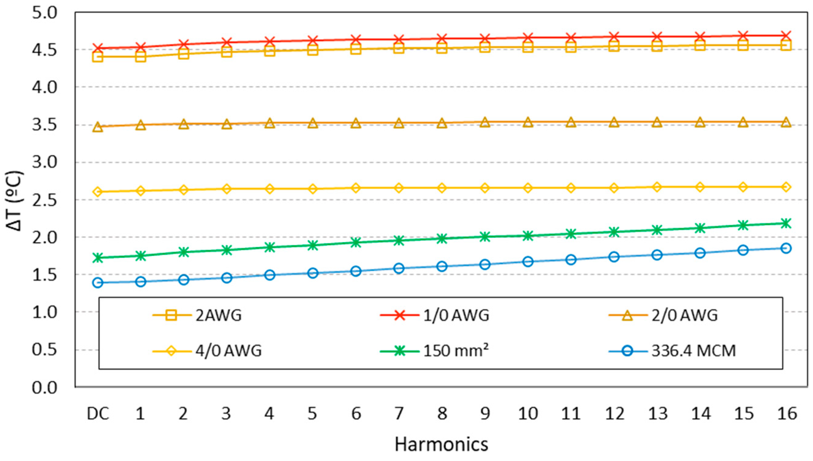
To examine the impact of temperature on the resistivity of the conductor $\left(\rho \right)$, the linear relationship between these two quantities was adopted as in reference [24]. Furthermore, reference [24] highlights that at lower temperatures, the correlation between temperature and electrical resistivity in aluminum alloys remains linear. Similarly, reference [25] also addresses this aspect. In the cases examined within this study, the maximum temperature increase was estimated to be approximately 5 °C, starting from an initial temperature of 20 °C. Additionally, it was observed that for thicker conductors, a temperature rise was noted as current frequency increased, as Figure 7 shows for 150 mm² and 336.4 MCM conductors. Meanwhile, the remaining conductors displayed a notable lower temperature increase with current frequency, which suggests that the skin effect results in significant heating for thicker conductors, considering current frequency increases.

It should be emphasized that the increase in temperature observed for harmonic components, compared to the temperature rise for DC current flowing through the conductor, is primarily caused by the skin effect. The recorded data regarding temperature rise for harmonic components are presented in

Table 2. Temperature rise due exclusively to skin effect.

Conductor	$∆\mathit{T}={\mathit{T}}_{16\mathit{h}\mathit{a}\mathit{r}\mathit{m}\mathit{o}\mathit{n}\mathit{i}\mathit{c}}-{\mathit{T}}_{\mathit{D}\mathit{C}}(°\mathbf{C})$	$\frac{\mathit{\rho }}{{\mathit{\rho }}_{\mathit{D}\mathit{C}}}\left(\mathbf{\%}\right)$
2 AWG—AAC	0.155	0.062
1/0 AWG—ASCR	0.159	0.064
2/0 AWG—AAC	0.070	0.028
4/0 AWG—AAC	0.067	0.027
150 mm2—AAC	0.464	0.187
336.4 MCM—ASCR	0.429	0.172

.

To specifically quantify the error resulting from temperature rise associated with the skin effect, Table 2 indicates that the largest error is observed for 150 mm²—the AAC conductor, with an error of 0.187% corresponding to a temperature rise of 0.464 °C. Another noteworthy aspect is that the skin effect is more prominent for thicker conductors, and Table 2 as well as Figure 7 showcase this result, as expected.

Therefore, based on the analysis of aluminum alloys used in the examined conductors, it is concluded that the relationship between temperature and electrical resistivity can be considered linear [23]. Furthermore, it is appropriate to model the resistivity by means of (25) to specify the percentage increment for resistivity $\frac{\rho }{{\rho }_{20°\mathrm{C}}}\times 100\%$.

$${\rho }_T={\rho }_{{Al}_{(20°C)}}\left[1+\alpha \left(T-T_0\right)\right]\left[\frac{\mathsf{\Omega }}{\mathrm{m}}\right]$$

(25)

Considering that $\alpha =0.00403\left(\raisebox{1ex}{$1$}\!\left/ \!\raisebox{-1ex}{$°\mathrm{C}$}\right.\right)$ [13] and ${\rho }_{{Al}_{(20°C)}}=61\%IACS\left(\mathsf{\Omega }·\mathrm{m}\right)$, as indicated by the manufacturer of the conductors [24], one can quantify how much the resistance of the conductors is influenced by the increase in resistivity due to temperature rise.

The results indicate that the temperature increase observed during the process of measuring conductor resistance, in the worst-case scenario (conductor 1/0 AWG—ACSR), leads to an error of 1.888% in the quantification of the resistance value. As expected, the 1/0 AWG—ACSR conductor has lower ampacity, and therefore experiences greater power dissipation through Joule’s effect. Additionally, its geometry includes steel reinforcement, which has a resistivity 20 times greater than typical aluminum alloys [24], resulting in greater heating during the measurement process.

To summarize the measured data, Table 1 shows an increase in electrical resistivity due to temperature rise. For DC, all of the conductors exhibited a maximum resistivity increase of 1.9%. This percentage remained consistent for both the fundamental frequency and all harmonic components.

Furthermore, Table 2 estimates an approximate 0.2% increase in electrical resistivity for the skin effect measurement due to temperature rise. However, this heating effect has a negligible impact on the conductor’s resistance measurement. In other words, the increase in electrical resistivity caused by the RMS values of the fundamental and harmonic components contributes to a 1.9% rise in resistivity, while the skin effect causes only a 0.2% increase, which is considered practically negligible.

Having discussed the measurement configuration for the skin effect and the variables that can introduce errors, the subsequent section will delve into the analysis of the measured data and their application to reduce simulation time for harmonic power flow studies.

4. Results and Discussion

4.1. Measurement Results—Skin Effect

Through performing tests, an increase in the resistance of the studied conductors was obtained, which considered the skin effect. Noteworthy here is that verification was sought for the DC resistances values of the conductors made available by the manufacturers [26,27] and as such, was confirmed by the measurement methodology proposed in this study. Therefore, the measured reference value was used to specify the start of the measurement process. From this value,

Table 3. Electrical resistances of conductors in direct current at 20 °C.

Conductor	${\mathit{R}}_{\mathit{m}\mathit{e}\mathit{a}\mathit{s}\mathit{u}\mathit{r}\mathit{e}\mathit{d}}$ $\left(\raisebox{1ex}{$\mathsf{\Omega }$}\!\left/ \!\raisebox{-1ex}{$\mathbf{k}\mathbf{m}$}\right.\right)$	${\mathit{R}}_{\mathit{d}\mathit{a}\mathit{t}\mathit{a}\mathit{s}\mathit{h}\mathit{e}\mathit{e}\mathit{t}}$ $\left(\raisebox{1ex}{$\mathsf{\Omega }$}\!\left/ \!\raisebox{-1ex}{$\mathbf{k}\mathbf{m}$}\right.\right)$	Error $\left(\mathbf{\%}\right)$
2 AWG—AAC	0.8652	0.8541	1.31
1/0 AWG—ASCR	0.5285	0.5360	1.40
2/0 AWG—AAC	0.4517	0.4550	0.72
4/0 AWG—AAC	0.2616	0.2676	2.21
150 mm2—AAC	0.2046	0.2060	0.64
336.4 MCM—ASCR	0.1726	0.1703	1.36

presents the measured resistance values in DC resistances.

The carried-out measurements showed errors of less than 2.5%, thus ensuring that the measurement process is adequate, these being the reference values used in Figure 8. Based on the measurement results, the theory is corroborated, in which thicker conductors are subject to a greater influence of the skin effect, as illustrated in Figure 8 for the 4/0 AWG, 150 mm² and 336.4 MCM conductors. In these conductors, a greater increase in electrical resistance was noted, which results from the skin effect. Furthermore, one notes that the 1/0 AWG conductor, although belonging to the conductors being tested with lower thickness, exhibited a relevant impact against the skin effect. In comparison, the 2 AWG conductor together with the 2/0 AWG, composed only of aluminum wires (AAC), exhibited the lowest influence from the skin effect. From Figure 8, verification was made that the conductors that presented the greatest heating, such as 2 AWG and 1/0 AWG, stand out for showing an increasing tendency as the electrical current increases, indicating, through progressive 3D line graphs, the impact of temperature on the measurement process. Meanwhile, this behavior is not observed in the remainder of the conductors, since the range of test currents (20–40 A) is much lower than the ampacity of the conductors, highlighting, therefore, significantly lower heating of these conductors.

The comparison between the measurement results and the theoretical expectations is significant, as it provides insights into the behavior of the measured data, as displayed in Figure 9. Additionally, the magnitude of the resistance increase is an important aspect to consider. It was observed that for electric currents at 960 Hz, running through the conductor, an increase of around 60% was verified in the electrical resistanc, in comparison to DC resistance for the 1/0 AWG, 4/0 AWG, 150 mm² and 336.4 MCM conductors.

Against this backdrop, the following topics aim to quantitatively assess the impact that the skin effect has on power simulation studies, while considering distorted conditions of electric current and the measurement values obtained at this stage of the study.

4.2. Statistical Simplified Method to Estimate Skin Effect for Low Frequencies

To simplify the process and obtain a single resistance value per frequency, an averaging method was employed considering the variation in current in the conductor. For each frequency, the resistance values were synthesized to be considered, as pointed out in (26).

$$R_h=average\left(R_{20A},R_{22A},\cdots ,R_{40A}\right)$$

(26)

Based on this compilation, Figure 10 provides the values that were computed as a result of applying expression (26) to the data. Figure 10 shows that the conductors under test are appropriately estimated through a linear equation considering low frequencies. Not only are the expressions presented in Figure 10 simpler, but they also reduce the processing time when computing the skin effect. It should be emphasized that for harmonic power flow studies, especially those covering the distribution power network of an entire operator region, they may take up to 48 h of simulation time. To compare the time processing between Bessel’s proposed expression (22) adapted to 60 Hz resistance as a reference against the Figure 10 expressions, an algorithm in Python (PyCharm) was implemented. The results show that Bessel’s expression (22) required 53.85 ms to compute the skin effect for all conductors for the before mentioned frequency range, as opposed to 41.88 ms of simulation time for the Figure 10 expressions. Therefore, the reduction in simulation time is approximately 20% using the proposed method.

For the purposes of an objective assessment of the study, the IEEE 8500 node feeder [28], which is known throughout the scientific community, was used to calculate the power losses under distorted conditions. The studied feeder is shown in Figure 11, in which the line thickness for the segments corresponds to the regions where energy losses are more expressive. It is important to point out that information with greater detail on this feeder is available in [28].

Simulations were performed using OpenDSS and COM Interface with Python (PyCharm). To clearly meet the objective of this study, it was crucial to define the harmonic emissivity spectrum of the non-linear loads of this feeder. To this end, the use of input data from [29] was established for the frequency range of 60 Hz to 960 Hz. Another noteworthy aspect to mention is that additional conductors beyond the ones measured are present at the IEEE 8500 node feeder. To address this, an assumption was made to consider the behavior of the closest laboratory-tested conductor for these untested conductors.

To correctly estimate the time reduction for the harmonic power flow study, the two following separated conditions were performed:

Case 1: Bessel’s expression (22), adapted to 60 Hz resistance as a reference, as a correction factor for the skin effect $\left(\frac{R_f}{R_{60\mathrm{H}\mathrm{z}}}\right)$ applied to the resistance of line parameters, according to cables used at the transmission line, as expressed in (27).

Case 2: Figure 10 expressions as a correction factor for the skin effect applied $\left(\frac{R_f}{R_{60\mathrm{H}\mathrm{z}}}\right)$ to the resistance of line parameters, according to the cables used at the transmission line, as expressed in (27).

$$R_{{conductor}_f}=\frac{R_f}{R_{60\mathrm{H}\mathrm{z}}}{R}_{conductor}\left[\mathsf{\Omega }\right]$$

(27)

The simulation times of both conditions previously mentioned are shown in

Table 4. Simulation times spent for harmonic power flow study case.

Case 1	Case 2	Time Reduction	Percentage Reduction
279.64 s	231.25 s	48.39 s	17.30%

.

Another noteworthy aspect is the reliability of the results provided from the proposed method compared to Bessel’s expressions. Also, from a power systems perspective, power losses are segregated into several components, as illustrated in Figure 12. Skin effect losses are responsible for 4.00% of additional losses on the IEEE 8500 node test feeder.

5. Conclusions

The research conducted in this study offers a new perspective on the impact of the skin effect on conductors used in energy distribution networks, particularly in relation to Joule losses associated with this phenomenon. The study aimed to provide a mathematical understanding of the non-uniform current distribution in the cross-section of the conductor, thereby explaining its physical origin. A notable aspect of this research is the methodology developed for measuring the skin effect, which was applied to six commonly used conductors in energy distribution networks. The evaluation criteria used for measuring the electrical resistance of the conductors in direct current showed an error of less than 2.5% compared to the manufacturer’s specified values.

Furthermore, the study examined the behavior of conductor resistance under harmonic electric currents ranging from the 2nd to the 16th harmonic order, in order to assess the significance of the skin effect. It was observed that the impact of temperature rise on resistivity during the measurement process was 1.9% due to the heating effect caused by the current. Conversely, the temperature rise caused by the skin effect was less than 0.2%, which is considered negligible when it comes to resistance measurements.

After measuring the resistance of the conductors under each magnitude (20–40 A) and frequency (60–960 Hz), the IEEE 8500 node feeder was used to perform a harmonic power flow study. In this regard, it was noted that the proposed expressions provided a reduction in simulation time of approximately 17%, and the skin effect was responsible for a percentage of 4.00% in additional losses.

Hence, the studies conducted in this research aim to provide a practical perspective on a well-known phenomenon within the scientific community, specifically addressing the proposed expressions as a method to reduce simulation times for harmonic power flow studies.