Detection of False Data Injection Attacks in a Smart Grid Based on WLS and an Adaptive Interpolation Extended Kalman Filter

Abstract

An accurate power state is the basis of the normal functioning of the smart grid. However, false data injection attacks (FDIAs) take advantage of the vulnerability in the bad data detection mechanism of the power system to manipulate the process of state estimation. By attacking the measurements, then affecting the estimated state, FDIAs have become a serious hidden danger that affects the security and stable operation of the power system. To address the bad data detection vulnerability, in this paper, a false data attack detection method based on weighted least squares (WLS) and an adaptive interpolation extended Kalman filter (AIEKF) is proposed. On the basis of applying WLS and AIEKF, the Euclidean distance is used to calculate the deviation values of the two-state estimations to determine whether the current moment is subjected to a false data injection attack in the power system. Extensive experiments were conducted to simulate an IEEE-14-bus power system, showing that the adaptive interpolation extended Kalman filter can compensate for the deficiency in the bad data detection mechanism and successfully detect FDIAs.

1. Introduction

The modern power system is developing towards intelligence, and plenty of intelligent devices, such as smart meters and sensors, promote the transformation of the power system in the modes of power generation, transformation, transmission, and distribution, which makes the smart grid a typical cyber–physical system (CPS) [1,2]. In a smart grid, the supervisory control and data acquisition (SCADA) system collects and analyzes real-time data from field devices across the network. Finally, the SCADA reports back to the control center, which then makes adjustments to the power generation and distribution of the grid based on this information [3].

The susceptibility of the power cyber–physical system (CPS) to cyber attacks is a result of the unpredictable nature of sensor data in the perception layer and the unrestricted communication channels for data exchange [4,5]. Among the many types of cyber attacks, attacks against smart grids and industrial control systems are the most common; the damage caused to the system cannot be underestimated, seriously affecting the normal production activities of society. For example, in 2010, the “Stuxnet” virus attack on a Belarusian enterprise, which caused anomalies in uranium enrichment centrifuges and generators at the Iranian nuclear power plant, resulted in damage to many pieces of equipment [6]. In 2015, Black Energy, a cyber virus targeting the power grid, caused power outages at some Ukrainian power plants, disrupting the power supply to many factories in the Ivano-Frankivsk region and affecting production [7]. The investigation revealed that the incident resulted in the malicious deletion of historical grid measurements stored in the SCADA, which made recovery extremely difficult.

A false data injection attack (FDIA) is a novel attack method specifically targeting the integrity of state estimation data in the power CPS [8,9]. The attackers inject false data, which affects the power flow calculation, control decisions, etc., through smart grid sensors, controllers, and remote control units to tamper with the original data of the grid. This situation can potentially result in the malfunction of grid equipment and, in severe cases, the complete paralysis of the power network, which not only poses a significant threat to grid security but also carries the potential for substantial economic losses. 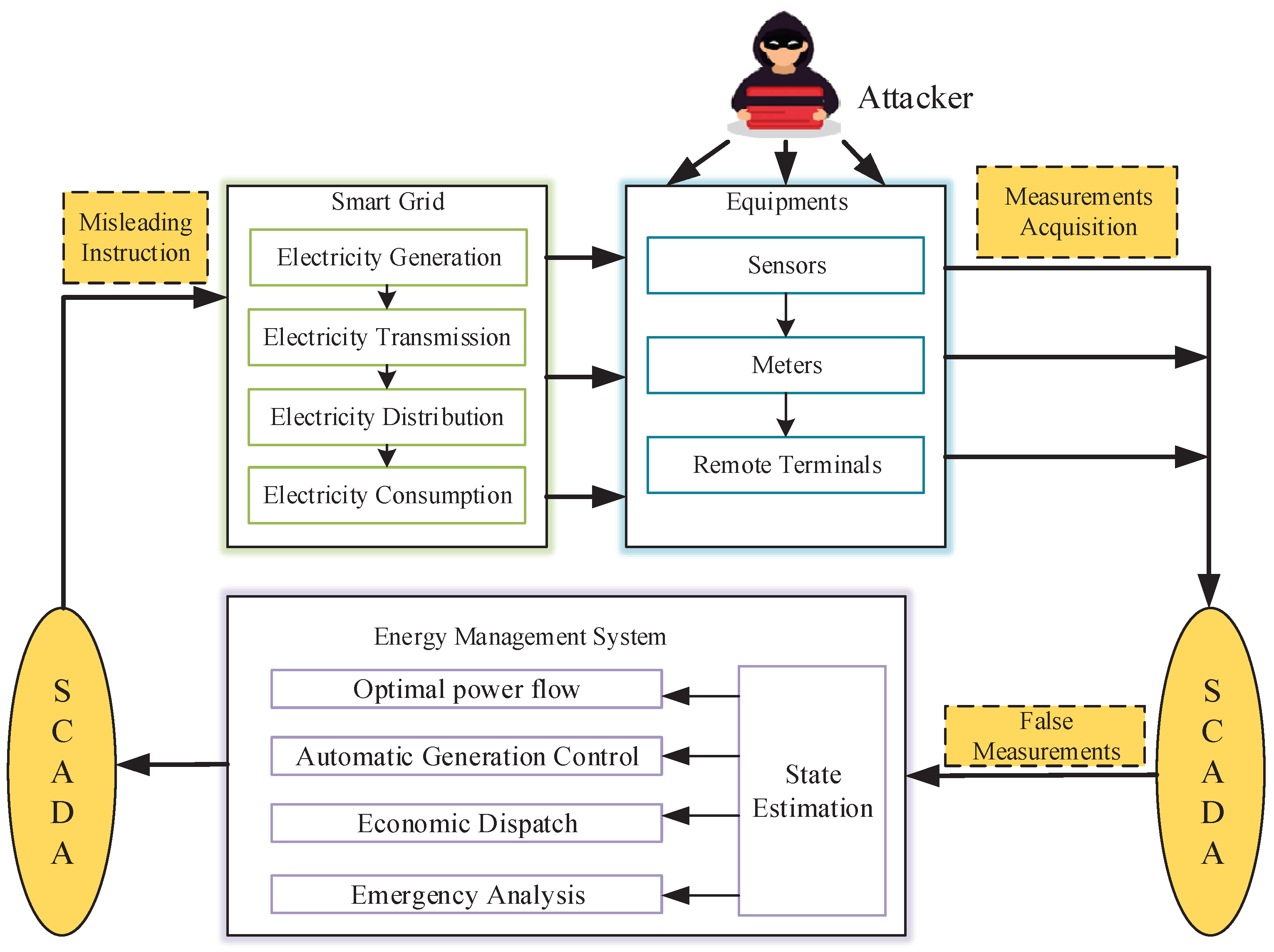Figure 1 shows the structure of a smart grid system and an illustration of an FDIA.

Liu et al. [10] first introduced the topic of FDIAs in the literature, where it was hypothesized that an attacker could access the current configuration information of a smart grid and manipulate meter or sensor measurements. Such an attack could insert false data into specific state variables, avoiding detection by current bad data detection algorithms. Yang et al. [11] delved into the challenge of determining the most effective attack strategy. This strategy, known as an injection attack strategy, involves selecting a specific set of meters to manipulate in a way that maximizes the resulting damage. They not only formalized this problem but also developed efficient algorithms to pinpoint the ideal set of meters for such attacks. It is important to highlight that even if these attacks are isolated to specific devices, their impact on the smart grid can be catastrophic due to the grid’s intricate interconnections. As described by He et al. [12], electricity theft by attackers by modifying smart meter data has seriously affected utility security. Therefore, many researchers have devoted themselves to the detection of false data injection attacks in order to safeguard the security of the smart grid.

When the power system is subjected to malicious false data injection, the state estimation result of the WLS under attack is updated in real time by incorporating an estimation algorithm of an extended Kalman filter, which has a hysteresis in its state estimation process, and by observing disparities in the estimation outcomes produced by the two algorithms, making it possible to detect the FDIA. Meanwhile, to improve the accuracy and reduce the linearization error of the EKF, the adaptive interpolation strategy is introduced. Therefore, in this paper, we propose a detection method based on WLS and AIEKF. Considering that the two algorithms have different degrees of correspondence to real-time information, the FDIA can be effectively detected. The main contributions can be summarized as follows:

• Considering the linearization error of the EKF algorithm in state estimation in a power system, the adaptive interpolation strategy is introduced. The pseudomeasurements between two consecutive measurements are inserted by linear interpolation to improve the estimation accuracy.
• We propose a novel FDIA detection method that combines AIEKF and WLS, marking the first instance of their joint application in this context.
• We conduct many experiments on an IEEE-14-bus power system to demonstrate the proposed algorithm’s performance in detecting FDIAs. The result shows that the method can effectively detect FDIAs.

The remainder of the paper is structured as follows. Section 2 provides an overview of relevant literature pertaining to the detection of FDIAs. Section 3 outlines the system model employed in this study. In Section 4, we delve into the details of the proposed AIEKF algorithm. In Section 5, the detection principle is described. The experiments and results are presented in Section 6. Finally, in Section 7, we present our concluding remarks and suggest directions for future work. A list of abbreviations and acronyms is provided in

Table 1. A list of abbreviations and acronyms.

Abbreviations and Acronyms	Full Name
AIEKF	Adaptive interpolation extended Kalman filter
BDD	Bad data detection
CPS	Cyber–physical system
EMS	Energy management system
FDIAs	False data injection attacks
LNR	Largest normalized residual
PMUs	Phase measurement units
RMSE	Root mean square error
SCADA	Supervisory control and data acquisition
WLS	Weighted least squares

.

2. Related Work

Since the concept of FDIAs was introduced, the issues related to FDIAs have received a great deal of attention in both academic research and industry. Many scholars have studied bad data in state estimation and proposed corresponding detection methods for FDIAs based on their research. Although FDIA detection algorithms differ from each other, the algorithms can be classified into two categories [13]: model-based algorithms and data-driven algorithms.

2.1. Model-Based Detection Algorithms

Nowadays, with the increasing degree of interconnection of power systems in smart grids, the simple use of weighted least squares is no longer applicable, and many variants have emerged. Moslemi et al. [14] introduced an innovative cyber attack detection technique based on maximum likelihood estimation. This method capitalizes on the near-chordal sparsity (NCS) characteristics of the power grid to establish a robust framework for addressing the corresponding maximum likelihood estimation problem. Furthermore, they broke down this detection approach into a series of localized maximum likelihood estimation problems. This approach not only safeguards privacy but also mitigates potential issues. Chen et al. [15] introduced a novel method for detecting FDIAs using kernel density estimation. This method utilizes the concept of kernel density estimation, which utilizes historical data to estimate the probability distributions of both measurements and control commands. Additionally, it calculates confidence intervals for these estimates at a specified significance level. Zhao et al. [16] proposed a method that employs short-term state prediction in smart grids to detect spurious data injection attacks. This method utilizes real-time and predicted states to pinpoint potential false data injections by analyzing the differences between them. By continuously monitoring and comparing the accuracy of short-term state predictions, this approach enhances the security and resilience of smart grid systems by improving the detection of malicious attacks. Li et al. [17] proposed a detection method based on the watermark embedding technique. The method uses a dynamic watermark embedding technique to embed security-enhancing markers (watermarks) into the grid measurement data to ensure the integrity and authenticity of the data. Then, the data embedded with the watermark are processed and detected using the EKF algorithm to identify possible faulty data insertion attacks. Through the joint application of dynamic watermarking and EKF, this method can improve the detection capability of smart grid systems against FDIAs and provide increased security. The above methods cannot be used alone; they must be used with the help of some determination methods to determine the existence of FDIAs. Some determination methods are available, such as Euclidean distance [16,18], maximum normalized residuals [19,20], chi-square testing [18,21], Cumulative sum testing [22,23], Kullback–Leibler distance [14,24], and cumulative error sum of squares probability density curves [25,26].

2.2. Data-Driven Detection Algorithms

In contrast to detection algorithms that rely on system models, data-driven detection algorithms operate without the need for system parameters and models. The process of detecting FDIAs is independent of these factors, and it relies on a large amount of historical data from the smart grid to speculate on future data [13]. Mahi-Al-Rashid et al. [27] proposed an innovative approach for countering FDIAs. They employed a CNN-LSTM-based self-encoder sequence-to-sequence architecture for prediction-assisted anomaly detection. Additionally, they suggested an adaptive optimal thresholding method based on consumption patterns to identify unusual behaviors. Yu et al. [28] proposed an online method for detecting FDIAs that merges wavelet transform with deep neural networks. This approach involves extracting features from grid sensor data using wavelet transform and subsequently employing a deep neural network for real-time detection. This methodology effectively enhances the security and reliability of the smart grid system by identifying potential attacks as they occur. Wang et al. [29] combined Kalman filtering with recurrent neural networks. The actual state of the grid was first estimated using Kalman filtering. Next, the estimated state was modeled and predicted using recurrent neural networks. By analyzing the disparity between the predicted state and the real measured data, the system can identify the existence of FDIAs. Jorjani et al. [30] introduced a novel algorithm designed for the detection of FDIAs in AC state estimation. This algorithm employs outlier detection techniques to the outcomes of state estimation because the attack may lead to data inconsistencies between buses, resulting in an abnormal graph structure. The above methods can be proven to detect FDIAs.

3. System Model

The state estimation of the power system usually deeply relies on the system model. The selection and establishment of the model have a substantial impact on the results of the system state calculation, which directly lead to the accuracy of the acquired state. State estimation in the power system is a crucial element within EMS, as it provides essential real-time information about the grid’s operational status, and it is the basis for other high-level applications to realize the calculation and analysis.

The measurements for power system state estimation are collected from the grid by SCADA or phase measurement units (PMUs). PMUs are able to provide accurate and synchronized phase measurements for geographically dispersed buses in the grid by taking advantage of the high accuracy, sub-microsecond time synchronization, and unprecedented reporting rate [31]. And if the system is completely observable with PMU measurements, the state estimation process is a linear procedure. The proposed algorithm aims at solving the linearization of EKF for state estimation. Therefore, the proposed algorithm can be applied to the mentioned PMU-based state estimation problem by reducing the linearization steps of the AIEKF algorithm. We can discuss a situation in which there are m measurements and n state variables. In an AC power system, the connection between measurements and state variables is characterized by a nonlinear relationship, which can be represented as:

$$\mathit{z}=h\left(\mathit{x}\right)+\mathit{e}$$

(1)

where $\mathit{z}\in {\mathbb{R}}^{m\times 1}$ is the measurement vector; $\mathit{x}\in {\mathbb{R}}^{n\times 1}$ is the state vector, typically bus voltage amplitude and phase; $\mathit{e}\in {\mathbb{R}}^{m\times 1}$ is the measurement error vector that satisfies $\mathit{e}={\left(e_1,e_2,\dots ,e_m\right)}^T\sim \mathcal{N}\left(0_{m\times 1},\mathit{R}\right)$; and $h(·)$ represents the nonlinear relationship between the measurement vector ($\mathit{z}$) and the state vector ($\mathit{x}$).

To analyze the correlation between the bus voltage, phase angle, and bus current of the grid system and determine the nonlinear relationship $h(·)$, we must streamline the power system branch by representing it through an equivalent circuit, as illustrated in Figure 2. Subsequently, utilizing the AC model of the power system, we establish the connection between the state variables and measurements, which can be formulated as follows:

$$P_i=V_i\sum _{j\in T}{V}_j\left[G_{ij}cos{\theta }_{ij}+B_{ij}sin{\theta }_{ij}\right]$$

(2)

$$Q_i=V_i\sum _{j\in T}{V}_j\left[G_{ij}sin{\theta }_{ij}-B_{ij}cos{\theta }_{ij}\right]$$

(3)

$$P_{ij}=V_i^2{G}_{ij}-V_i{V}_j\left[G_{ij}cos{\theta }_{ij}+B_{ij}sin{\theta }_{ij}\right]$$

(4)

$$Q_{ij}=-V_i^2{B}_{ij}-V_i{V}_j\left[G_{ij}sin{\theta }_{ij}-B_{ij}cos{\theta }_{ij}\right]$$

(5)

where $V_i$ and $V_j$ are the voltage amplitudes at bus i and bus j, respectively; $P_i$ and $Q_i$ represent the active and reactive power injection of bus i, respectively; $P_{ij}$ and $Q_{ij}$ denote active power flow and reactive power flow from bus i to bus j, respectively; $G_{ij}$ and $B_{ij}$ denote the conductance and susceptance of the line from bus i to bus j, respectively; ${\theta }_{ij}$ denotes the phase angle difference of the line voltage from bus i to bus j; and T denotes the set buses adjacent to bus i.

3.1. State Estimation

The most commonly used state estimation in power systems is the weighted least squares method, which is still widely used [32,33,34]. Under this method, the objective function ($\mathit{J}\left(\widehat{\mathit{x}}\right)$) is the weighted sum of squares of the difference between the measured and estimated values. With the smallest objective function value, the obtained $\mathit{x}$ is the closest approximation to the true state of the system. Based on the weighted least squares method, the objective function ($\mathit{J}\left(\widehat{\mathit{x}}\right)$) can be expressed as:

$$\mathit{J}\left(\widehat{\mathit{x}}\right)={\left[\mathit{z}-\mathit{h}\left(\widehat{\mathit{x}}\right)\right]}^T{\mathit{R}}^{-1}\left[\mathit{z}-\mathit{h}\left(\widehat{\mathit{x}}\right)\right].$$

(6)

Then,

$$\widehat{\mathit{x}}=argmin{\left[\mathit{z}-\mathit{h}\left(\widehat{\mathit{x}}\right)\right]}^T{\mathit{R}}^{-1}\left[\mathit{z}-\mathit{h}\left(\widehat{\mathit{x}}\right)\right]$$

(7)

To solve the nonlinear WLS problem, we can linearize the measurement equation around $\mathit{x}$, then apply the linear WLS method. The final result is expressed as:

$${\widehat{\mathit{x}}}^{k+1}={\widehat{\mathit{x}}}^k+{\left[G\left({\widehat{\mathit{x}}}^k\right)\right]}^{-1}{\mathit{H}}^{\mathit{T}}\left({\widehat{\mathit{x}}}^k\right){\mathit{R}}^{-1}\left(\mathit{z}-\mathit{h}\left({\widehat{\mathit{x}}}^k\right)\right)$$

(8)

$$G\left({\widehat{\mathit{x}}}^k\right)={\mathit{H}}^{\mathit{T}}\left({\widehat{\mathit{x}}}^k\right){\mathit{R}}^{-1}\mathit{H}\left({\widehat{\mathit{x}}}^k\right)$$

(9)

where k is the k-th iteration index, and $\mathit{H}\in {\mathbb{R}}^{m\times n}$ is the Jacobian matrix of the measurement equation, which can be expressed as:

$$\mathit{H}={\left[\begin{array}{cccc}\begin{array}{cc}\begin{array}{c}\frac{\partial V_i}{\partial V}\\ \\ \frac{\partial V_i}{\partial \theta }\end{array}& \begin{array}{c}\frac{\partial P_i}{\partial V}\\ \\ \frac{\partial P_i}{\partial \theta }\end{array}\end{array}& \begin{array}{c}\frac{\partial Q_i}{\partial V}\\ \\ \frac{\partial Q_i}{\partial \theta }\end{array}& \begin{array}{c}\frac{\partial P_{ij}}{\partial V}\\ \\ \frac{\partial P_{ij}}{\partial \theta }\end{array}& \begin{array}{c}\frac{\partial Q_{ij}}{\partial V}\\ \\ \frac{\partial Q_{ij}}{\partial \theta }\end{array}\end{array}\right]}^T$$

(10)

3.2. Bad Data Detection

Traditional methods for detecting bad data, like the chi-square test and largest normalized residual (LNR) test, rely on the results obtained from WLS estimation.

By checking the value of the objective function ($\mathit{J}\left(\widehat{\mathit{x}}\right)$), we can determine whether there are bad data in the power system or not. In particular, in the chi-square test, we need to perform null hypothesis testing, which can be expressed as:

$$\left\{\begin{array}{c}\mathit{J}\left(\widehat{\mathit{x}}\right)>{\chi }_{\left(m-n\right),p}^2,\mathrm{Reject}{\mathit{H}}_0\\ \mathit{J}\left(\widehat{\mathit{x}}\right)\le {\chi }_{\left(m-n\right),p}^2,Accept{\mathit{H}}_0\end{array}\right.$$

(11)

where ${\mathit{H}}_0$ represents the original hypothesis, i.e., there are no bad data, and ${\chi }_{\left(m-n\right),p}^2$ is the chi-square test threshold with a confidence level of p and a degree of freedom corresponding to $\left(m-n\right)$.

The LNR test stands as another commonly employed approach for bad data detection. Its core concept revolves around the normalization of measurement residuals, which can be formulated as follows:

$$r_i=\frac{\left|z_i-h_i\left(\widehat{x}\right)\right|}{\sqrt{{\mathsf{\Omega }}_{ii}}}$$

(12)

$$\mathsf{\Omega }=\left[\mathit{I}-\mathit{H}\left(\widehat{x}\right){\left({\mathit{H}}^{\mathit{T}}\left(\widehat{\mathit{x}}\right){\mathit{R}}^{-1}\mathit{H}\left(\widehat{x}\right)\right)}^{-1}{\mathit{H}}^{\mathit{T}}\left(\widehat{\mathit{x}}\right){\mathit{R}}^{-1}\right]\mathit{R}$$

(13)

where $z_i$ is the ith measurement, ${\mathsf{\Omega }}_{ii}$ is the ith diagonal entry of $\mathsf{\Omega }$, and $\mathit{I}$ is the identity matrix. If there exit bad data in the power system, the largest normalized residual is larger than the threshold ($\epsilon$).

The chi-square test and LNR test are generally effective for detecting natural bad data, which typically induce large measurement residuals [35].

3.3. FDIA Generation

If an attacker possesses precise information regarding real-time state estimation, network topology, and parameters, they can achieve an elaborate FDIA without being detected. When measurement meters are tampered with, the measurement ($\mathit{z}$) changes to ${\mathit{z}}^f$, and the attacked measurement (${\mathit{z}}^f$) changes to:

$${\mathit{z}}^f=\mathit{h}\left(\mathit{x}\right)+\mathit{a}+\mathit{e}$$

(14)

where $\mathit{a}\in {\mathbb{R}}^{m\times 1}$ is the attacked vector.

As an elaborate FDIA, the attacked vector requires a certain condition, which is expressed as:

$$\mathit{a}=\mathit{h}(\widehat{\mathit{x}}+\mathit{c})-\mathit{h}\left(\widehat{\mathit{x}}\right)$$

(15)

where $\mathit{c}\in {\mathbb{R}}^{n\times 1}$ is the deviation of the state variable, and $\widehat{\mathit{x}}$ is the state-estimated vector without an FDIA.

As indicated by the equation above, FDIAs can lead to an identical measurement residual vector compared to the condition without an attack. To be specific, the measurement residuals between the pre-attack and post-attack states can be described as follows:

$$\mathit{r}=\mathit{z}-\mathit{h}\left(\widehat{\mathit{x}}\right)$$

(16)

$${\mathit{r}}^{\mathit{f}}={\mathit{z}}^{\mathit{f}}-\mathit{h}(\widehat{\mathit{x}}+\mathit{c})=\mathit{z}+\mathit{a}-\mathit{h}\left(\widehat{\mathit{x}}\right)-\mathit{a}=\mathit{z}-\mathit{h}\left(\widehat{\mathit{x}}\right)$$

(17)

The measurement residual between the pre-attack and post-attack states does not change; hence, an elaborate FDIA is stealthy and can avoid detection by the existing BDD system based on residuals [36].

4. Dynamic State Estimation Model

4.1. Extended Kalman Filter (EKF)

The physical power information system in an AC power system is inherently complex and highly multidimensional and nonlinear. The state and measurement equations for state estimation can be formalized as:

$${\mathit{x}}_{\mathit{k}}=\mathit{f}\left({\mathit{x}}_{\mathit{k}-\mathbf{1}}\right)+{\mathit{\omega }}_{\mathit{k}-\mathbf{1}}$$

(18)

$${\mathit{z}}_{\mathit{k}}=\mathit{h}\left({\mathit{x}}_{\mathit{k}}\right)+{\mathit{e}}_{\mathit{k}}$$

(19)

where ${\mathit{x}}_{\mathit{k}}$ and ${\mathit{z}}_{\mathit{k}}$ denote the state vector and the measurement vector at time k, respectively; $\mathit{f}\left(.\right)$ denotes the state transfer equation from $k-1$ to k; $\mathit{h}\left(.\right)$ denotes measurement equation; and ${\mathit{\omega }}_{\mathit{k}-\mathbf{1}}$ and ${\mathit{e}}_{\mathit{k}}$ denote the process and measurement noise, respectively, which are independent of each other.

Since the KF algorithm can only deal with linear system problems, it is not applicable to nonlinear problems such as power systems, so the EKF algorithm is derived. The EKF algorithm first uses Taylor’s formula to linearize the nonlinear system, then filters it using the basic formula of the KF algorithm. Specifically, state Equation (18) carries out Taylor series expansion at the state estimation quantity (${\widehat{\mathit{x}}}_{\mathit{k}-\mathbf{1}}$) and ignores items at quadratic levels and higher. Similarly, measurement Equation (19) carries out Taylor series expansion at the state prediction quantity (${\tilde{\mathit{x}}}_{\mathit{k}}$) and ignores items at quadratic levels and higher. The linearization models are expressed as:

$$\begin{array}{c}{\mathit{x}}_{\mathit{k}}\approx \mathit{f}\left({\widehat{\mathit{x}}}_{k-1}\right)+{\left.\frac{\partial \mathit{f}\left({\widehat{\mathit{x}}}_{\mathit{k}-\mathbf{1}}\right)}{\partial {\widehat{\mathit{x}}}_{k-1}}\right|}_{{\widehat{\mathit{x}}}_{k-1}}\left({\mathit{x}}_{\mathit{k}-\mathbf{1}}-{\widehat{\mathit{x}}}_{k-1}\right)+{\mathit{\omega }}_{\mathit{k}-\mathbf{1}}\hfill \\ ={\mathit{F}}_{\mathit{k}-\mathbf{1}}{\mathit{x}}_{\mathit{k}-\mathbf{1}}+{\mathit{\omega }}_{\mathit{k}-\mathbf{1}}+{\mathit{u}}_{\mathit{k}-\mathbf{1}}\hfill \end{array}$$

(20)

$$\begin{array}{c}{\mathit{z}}_{\mathit{k}}\approx \mathit{h}\left({\tilde{\mathit{x}}}_k\right)+{\left.\frac{\partial \mathit{h}\left({\tilde{\mathit{x}}}_{\mathit{k}}\right)}{\partial {\tilde{\mathit{x}}}_{\mathit{k}}}\right|}_{{\tilde{\mathit{x}}}_k}\left({\mathit{x}}_{\mathit{k}}-{\tilde{\mathit{x}}}_k\right)+{\mathit{e}}_{\mathit{k}}\hfill \\ ={\mathit{H}}_{\mathit{k}}{\mathit{x}}_{\mathit{k}}+{\mathit{e}}_{\mathit{k}}+{\mathit{y}}_{\mathit{k}}\hfill \end{array}$$

(21)

where ${\mathit{F}}_{\mathit{k}-\mathbf{1}}={\left.\frac{\partial \mathit{f}\left({\widehat{\mathit{x}}}_{k-1}\right)}{\partial {\widehat{\mathit{x}}}_{k-1}}\right|}_{{\widehat{\mathit{x}}}_{k-1}}$ is the Jacobian matrix of the state equation, ${\mathit{u}}_{\mathit{k}-\mathbf{1}}=\mathit{f}\left({\widehat{\mathit{x}}}_{k-1}\right)-{\left.\frac{\partial \mathit{f}\left({\widehat{\mathit{x}}}_{k-1}\right)}{\partial {\widehat{\mathit{x}}}_{k-1}}\right|}_{{\widehat{\mathit{x}}}_{k-1}}{\widehat{\mathit{x}}}_{k-1}$ is an externality item, ${\mathit{H}}_k={\left.\frac{\partial \mathit{h}\left({\tilde{\mathit{x}}}_k\right)}{\partial {\tilde{\mathit{x}}}_k}\right|}_{{\tilde{\mathit{x}}}_k}$ is the Jacobian matrix of the measurement equation, and ${\mathit{y}}_{\mathit{k}}=\mathit{h}\left({\tilde{\mathit{x}}}_k\right)-{\left.\frac{\partial \mathit{h}\left({\tilde{\mathit{x}}}_k\right)}{\partial {\tilde{\mathit{x}}}_k}\right|}_{{\tilde{\mathit{x}}}_k}{\tilde{\mathit{x}}}_k$ is an externality item.

On the basis of Equations (18) and (19), the basic formula of the EKF algorithm is expressed as follows:

(1) Prediction steps:

$${\tilde{\mathit{x}}}_{k|k-1}={\mathit{F}}_{k-1}{\widehat{\mathit{x}}}_{k-1}$$

(22)

$${\tilde{\mathit{P}}}_{k|k-1}={\mathit{F}}_{k-1}{\widehat{\mathit{P}}}_{k-1}{\mathit{F}}_{k-1}^T+{\mathit{Q}}_{k-1}$$

(23)

(2) Update steps:

$${\mathit{K}}_k={\tilde{\mathit{P}}}_{k|k-1}{{\mathit{H}}_k}^T{({\mathit{H}}_k{\tilde{\mathit{P}}}_{k|k-1}{{\mathit{H}}_k}^T+{\mathit{R}}_k)}^{-1}$$

(24)

$${\widehat{\mathit{x}}}_k={\tilde{\mathit{x}}}_{k|k-1}+{\mathit{K}}_k\left[{\mathit{z}}_k-{\mathit{H}}_k{\tilde{\mathit{x}}}_{k|k-1}\right]$$

(25)

$${\widehat{\mathit{P}}}_k=\left(\mathit{I}-{\mathit{K}}_k{\mathit{H}}_k\right){\tilde{\mathit{P}}}_{k|k-1}$$

(26)

where $\tilde{}$ and $\widehat{}$ indicate the predicted and estimated quantities, respectively; $\mathit{I}$ is the identity matrix; $\mathit{P}$ is the state covariance matrix; $\mathit{Q}$ and $\mathit{R}$ are the covariance matrices of the process noise and measurement noise error vectors, respectively, which are assumed to be white Gaussian processes; and $\mathit{K}$ is Kalman gain.

The EKF algorithm is extensively employed for dynamic state estimation in power systems due to its straightforward model development and efficient computational performance in practical engineering applications. However, since the EKF algorithm ignores the higher-level items in the linearization process, it results in a large truncation error in power systems with highly nonlinear characteristics, resulting in a decrease in the filtering effect.

4.2. Adaptive Interpolation Strategy

To enhance the dynamic state estimation capabilities of the EKF algorithm in the power system, an adaptive interpolation method is proposed to strike a balance between estimation precision and computational efficiency [37].

Based on Equation (18), we need to quantify the nonlinear index of state function $\mathit{f}\left(\mathit{x}\right)$ to obtain ${\eta }_f$, which can be expressed as:

$${\mathit{\epsilon }}_{\mathit{f}}={\mathit{x}}_{\mathit{k}}-\mathit{f}\left({\widehat{\mathit{x}}}_{k-1}\right)-{\left.\frac{\partial \mathit{f}\left({\widehat{\mathit{x}}}_{\mathit{k}-\mathbf{1}}\right)}{\partial {\widehat{\mathit{x}}}_{k-1}}\right|}_{{\widehat{\mathit{x}}}_{k-1}}\left({\mathit{x}}_{\mathit{k}-\mathbf{1}}-{\widehat{\mathit{x}}}_{k-1}\right)$$

(27)

$${\eta }_f={{\mathit{\epsilon }}_{\mathit{f}}}^T{\mathit{Q}}_k^{-1}{\mathit{\epsilon }}_{\mathit{f}}$$

(28)

where ${\mathit{\epsilon }}_{\mathit{f}}$ is the difference between $\mathit{f}\left(\mathit{x}\right)$ and the corresponding linear approximation.

Similarly, based on Equation (19), we can obtain the nonlinear index (${\eta }_h$) of measurement function $\mathit{h}\left(\mathit{x}\right)$, which can be represented as:

$${\mathit{\epsilon }}_{\mathit{h}}={\mathit{z}}_{\mathit{k}}-\mathit{h}\left({\tilde{\mathit{x}}}_k\right)-{\left.\frac{\partial \mathit{h}\left({\tilde{\mathit{x}}}_{\mathit{k}}\right)}{\partial {\tilde{\mathit{x}}}_k}\right|}_{{\tilde{\mathit{x}}}_k}\left({\mathit{x}}_{\mathit{k}}-{\tilde{\mathit{x}}}_k\right)$$

(29)

$${\eta }_h={{\mathit{\epsilon }}_{\mathit{h}}}^T{\mathit{R}}_k^{-1}{\mathit{\epsilon }}_{\mathit{h}}$$

(30)

where ${\mathit{\epsilon }}_{\mathit{h}}$ is the difference between $\mathit{h}\left(\mathit{x}\right)$ and the corresponding linear approximation.

As shown in Equations (28) and (30), ${\mathit{\epsilon }}_{\mathit{f}}$ and ${\mathit{\epsilon }}_{\mathit{h}}$ are normalized by ${\mathit{Q}}_k$ and ${\mathit{R}}_k$. Under the process, ${\mathit{\epsilon }}_{\mathit{f}}$ and ${\mathit{\epsilon }}_{\mathit{h}}$ are numerically non-negative. Hence, if ${\mathit{\epsilon }}_{\mathit{f}}\ll {\mathit{Q}}_k$ and ${\mathit{\epsilon }}_{\mathit{h}}\ll {\mathit{R}}_k$, ${\eta }_f$ and ${\eta }_h$ are both much less than 1, and the system can be considered quasilinear. Otherwise, according to the size of the nonlinearization index, the pseudomeasurements must be added between two consecutive sampling points to increase the sampling rate and reduce the degree of nonlinearity of the system.

The interpolation factor (r) is closely related to the sizes of ${\mathit{\epsilon }}_{\mathit{f}}$ and ${\mathit{\epsilon }}_{\mathit{h}}$. The larger nonlinearization indices ${\eta }_f$ and ${\eta }_h$ are, the larger the interpolation factor (r) is. Conversely, the interpolation factor (r) is smaller. It is important to emphasize that ${\mathit{\epsilon }}_{\mathit{f}}=0$ and ${\mathit{\epsilon }}_{\mathit{h}}=0$ in the linear system. Therefore, the system does not interpolate.

The finite state machine model is shown in Figure 3. In practical applications, we can introduce as many states as required to the FSM model to accommodate the nonlinearity indices. There are three parameters in each state (i): the interpolation factor ($r_i$), the upper threshold ($U_i$), and the lower threshold ($L_i$). In addition, as the state (i) changes, the interpolation factor is set to $r_{i+1}>r_i$. The selection of the interpolation factor (r) is shown in Algorithm 1.

The thresholds of each state are different, and they are set depending on different scenarios. When selecting the thresholds, it is necessary to ensure that the upper threshold ($U_i$) is larger than the lower threshold ($L_i$). Furthermore, as $U_i$ and $L_i$ become smaller, the interpolation factor (r) and estimation accuracy increase, and the algorithm consumes more time. It is important to highlight that the nonlinear indices can take on discrete values. To maintain small values for both ${\mathit{\eta }}_{\mathit{f}}$ and ${\mathit{\eta }}_{\mathit{h}}$, here is how the process works: If either ${\mathit{\eta }}_{\mathit{f}}$ or ${\mathit{\eta }}_{\mathit{h}}$ exceeds $U_i$, r parameter is increased to minimize the nonlinear error. Conversely, if both ${\mathit{\eta }}_{\mathit{f}}$ and ${\mathit{\eta }}_{\mathit{h}}$ are below $L_i$, r is reduced to lower computational complexity. The specific values of r for each state can be found in

Table 2. The size of the interpolation factor (r).

State (i)	Interpolation Factor (r)	Lower Threshold	Upper Threshold
$i=1$	1	$L_1$	$U_1$
$i=2$	3	$L_2$	$U_2$
$i=3$	7	$L_3$	$U_3$
$i=4$	15	$L_4$	$U_4$

.

Algorithm 1 Choose the interpolation factor (r).

State $\mathit{i}$             $r=r_i$ if  ${\eta }_{fi}\mathrm{or}{\eta }_{hi}>U_i$  then     go to the state $\mathit{i}+\mathbf{1}$ else    ${\eta }_{fi}\mathrm{and}{\eta }_{hi}<L_i$     go to the state $\mathit{i}-\mathbf{1}$ end if Stay in the state $\mathit{i}$

4.3. Adaptive Interpolation EKF (AIEKF)

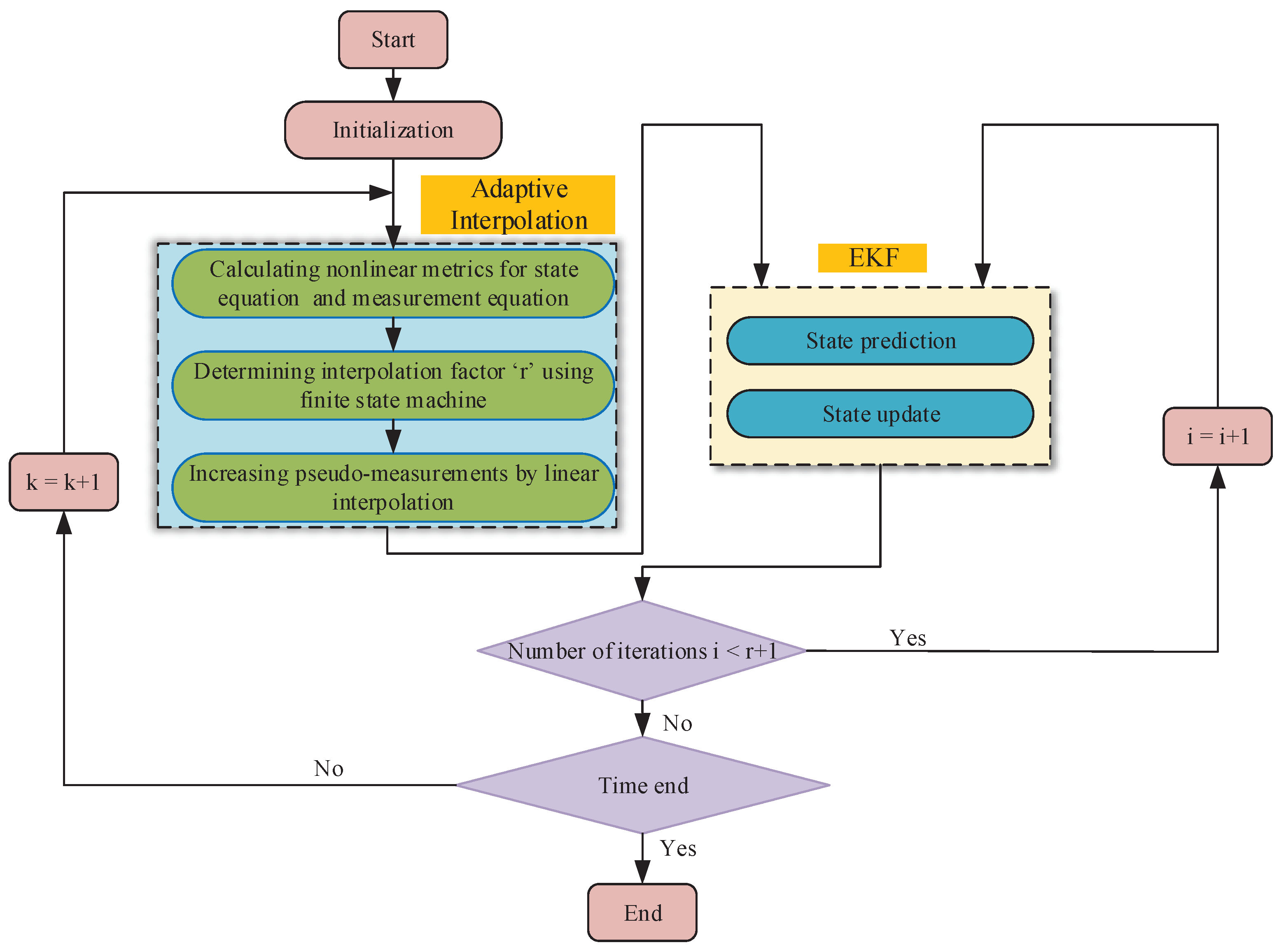
Building upon the dynamic model outlined in Section 4.1 and the adaptive interpolation approach discussed in Section 4.2, we introduce the AIEKF algorithm in this section. The AIEKF algorithm effectively strikes a balance between computation time and estimation accuracy, thereby enhancing the performance of the EKF algorithm in power systems. A flow chart illustrating the AIEKF algorithm is provided in Figure 4, and its detailed steps are as outlined as follows:

(1) Initialization: setting the initial state variable (${\widehat{\mathit{x}}}_{\mathbf{0}}$) and state error covariance (${\widehat{\mathit{P}}}_{\mathbf{0}}$).

(2) Adaptive Interpolation: In order to strike a compromise between computational efficiency and estimation precision, the algorithm incorporates an adaptive interpolation strategy, which comprises three key steps. Initially, we calculate the nonlinearity indices of the state transition function and the measurement function (referred to as ${\eta }_f$ and ${\eta }_h$, respectively) using Equations (28) and (30), respectively. In the next step, we ascertain the interpolation factor (r) by utilizing a finite-state machine model. Finally, r pseudomeasurements are introduced between two actual measurements through linear interpolation, which is designed to mitigate the adverse impacts of nonlinearity.

(3) EKF: On the basis of determining the number of interpolation factors (r), the power system is estimated using the EKF algorithm. Initially, leveraging the state and its covariance matrix from time $k-1$, we derive a prior estimation at time k in accordance with Equations (22) and (23). Secondly, the correction of the a priori estimation is used to obtain an a posteriori estimation according to Equations (24)–(26). Thirdly, filtering is performed between two consecutive samples based on the size of the interpolation factor. Then, the above steps are repeated until the end of the sampling time.

5. Detection of FDIAs

This section proposes a methodology for FDIA detection based on power system state estimation. As a nonlinear system in the smart grid, it is difficult to guarantee the estimation accuracy using traditional state estimation methods. Meanwhile, in order to improve the stability of the detection algorithm, the real-time state information of the grid buses is solved according to the system model equation and AIEKF algorithm.

Once the attacker begins to tamper with the measuring instruments, the result of Equation (25) is different from the previous result and expressed as:

$$\begin{array}{c}{\widehat{\mathit{x}}}_k^f={\tilde{\mathit{x}}}_{k\left|k-1\right.}+{\mathit{K}}_k[{\mathit{z}}_k+{\mathit{a}}_k-{\mathit{H}}_k{\tilde{\mathit{x}}}_{k\left|k-1\right.}]\hfill \\ \\ ={\widehat{\mathit{x}}}_k+{\mathit{K}}_k{\mathit{a}}_k\hfill \end{array}$$

(31)

where ${\widehat{\mathit{x}}}_{\mathit{k}}^{\mathit{f}}$ is the estimated state after the FDIA. To better facilitate estimation, ${\mathit{c}}_k={\widehat{\mathit{x}}}_{\mathit{k}}^{\mathit{f}}-{\widehat{\mathit{x}}}_k$ is introduced. Then, for the next time ($k+1$), it can be represented as:

$$\begin{array}{c}{\widehat{\mathit{x}}}_{k+1}^f={\tilde{\mathit{x}}}_{k+1\left|k\right.}^f+{\mathit{K}}_{k+1}[{\mathit{z}}_{k+1}^f-{\mathit{H}}_{k+1}{\tilde{\mathit{x}}}_{k+1\left|k\right.}^f]\hfill \\ ={\tilde{\mathit{x}}}_{k+1\left|k\right.}^f+{\mathit{K}}_{k+1}[{\mathit{z}}_{k+1}+{\mathit{a}}_{k+1}-{\mathit{H}}_{k+1}{\tilde{\mathit{x}}}_{k+1\left|k\right.}^f]\hfill \\ ={\widehat{\mathit{x}}}_{k+1}+\left[\mathit{I}-{\mathit{K}}_{k+1}{H}_{k+1}\right]{\mathit{F}}_k{\mathit{c}}_k+{\mathit{K}}_{k+1}{\mathit{a}}_{k+1}\hfill \end{array}$$

(32)

The analysis above highlights that the injection bias is influenced by both the currently injected false data and the bias present in the previously estimated state. Over time, this injection bias accumulates and gradually shifts the estimated state closer to the actual system state. When the power system is subjected to an FDIA, the altered measurements make the WLS state estimation results swing towards the new mean. For the AIEKF algorithm, due to the constraints of the state transfer matrix and the fact that its estimation is jointly determined by the predicted and measured values, the state estimation has some hysteresis, and only small oscillations occur.

Based on WLS and AIEKF estimation results, considering the influence of bus states on the system, the Euclidean distance in multidimensional spaces is introduced. The Euclidean distance detection threshold required in FDIA detection is obtained from historical data, and the Euclidean distance between two points estimated by WLS and AIEKF states is calculated online in real time and used as the basis for attack detection. The expression for the Euclidean distance at time k is expressed as follows:

$$d\left(k\right)=\sqrt{\sum _{i=1}^n{\left({\widehat{\mathit{x}}}_{i,k}^{WLS}-{\widehat{\mathit{x}}}_{i,k}^{AIEKF}\right)}^2}$$

(33)

where ${\widehat{\mathit{x}}}_{i,k}^{WLS}$ denotes the WLS-based state estimation at time k, ${\widehat{\mathit{x}}}_{i,k}^{AIEKF}$ denotes the AIEKF-based state estimation, and n denotes the system dimension.

In the n-dimensional grid system state space, the Euclidean distance is employed to quantify the spatial separation between two points within the same state space at a given time point. The Euclidean distance of the two state estimation algorithms stabilizes in a certain range during regular power system operation, which provides a basis for false data injection attack detection. The detection threshold is expressed as:

$${\tau }_D=max\left\{d\left(1\right),\dots ,d\left(n\right),\dots \right\}+\mu$$

(34)

where $\mu$ is the threshold margin, which is introduced to prevent false alarms triggered by minor data fluctuations while the detection system is operating under normal conditions.

Attack detection is performed by comparing the Euclidean distance between the detection threshold and the two points in the state space, and when $d\left(k\right)\ge {\tau }_D$, it is considered that there exits an FDIA in the power system; otherwise, it is considered that no attack occurs. The relation can be expressed as:

$$\left\{\begin{array}{c}d\left(k\right)<{\tau }_D,NoFDIA\\ d\left(k\right)\ge {\tau }_D,FDIA\end{array}\right.$$

(35)

In order to distinguish between bad data and FDIAs, bad data detection is also required at the end of the above steps. Only if $d\left(k\right)\ge {\tau }_D$ and $J\left(\widehat{x}\right)<{\chi }_{\left(m-n\right),p}^2$ hold can we conclude that the power system is under FDIAs. The proposed FDIA detection method based on WLS and AIEKF is shown in Algorithm 2.

Algorithm 2 FDIA detection based on WLS and the AIEKF algorithm

1: Initialize state variable ${\widehat{\mathit{x}}}_{\mathit{k}-\mathbf{1}}$ and state error covariance ${\widehat{\mathit{P}}}_{\mathit{k}-\mathbf{1}}$; the Euclidean distance detection threshold ${\tau }_D$; 2: Obtain the measurements by SCADA at time k; 3: In traditional static state estimation, WLS is widely used to calculate an estimated state vector ${{\widehat{\mathit{x}}}_{\mathit{k}}}^{WLS}$, ${\widehat{\mathit{x}}}_k^{WLS}={\left({\mathit{H}}_k^T{\mathit{R}}_k^{-1}{\mathit{H}}_{\mathit{k}}\right)}^{-1}{\mathit{H}}_k^T{\mathit{R}}_k^{-1}{\mathit{z}}_{\mathit{k}}$ 4: AIEKF (1) Calculate calculate the nonlinearity indices of the state transition function and the measurement function (referred to as ${\eta }_f$ and ${\eta }_h$) using Equations (28) and (30); (2) Ascertain the interpolation factor r by utilizing a finite state machine model; (3) Interpolate r pseudo-measurement between two actual measurements through linear interpolation; (4) Execute the state prediction step of the EKF by applying Equations (22) and (23); (5) Conduct the measurement update step of EKF by applying Equations (24)–(26) to calculate estimated state vector ${\widehat{\mathit{x}}}_k^{AIEKF}$, ${\widehat{\mathit{x}}}_k^{AIEKF}={\tilde{\mathit{x}}}_{k|k-1}+{\mathit{K}}_k\left[{\mathit{z}}_k-{\mathit{H}}_k{\tilde{\mathit{x}}}_{k|k-1}\right]$ 5: Calculate the Euclidean distance between two points estimated by WLS and AIEKF states; 6: if $d\left(k\right)\ge {\tau }_D$ and $J\left(\widehat{x}\right)<{\chi }_{\left(m-n\right),p}^2$ then 7:    Exist FDIA and generate early warning; 8: else 9:    Continue the state estimation process at time $k=k+1$, 10: end if

6. Experiments and Results

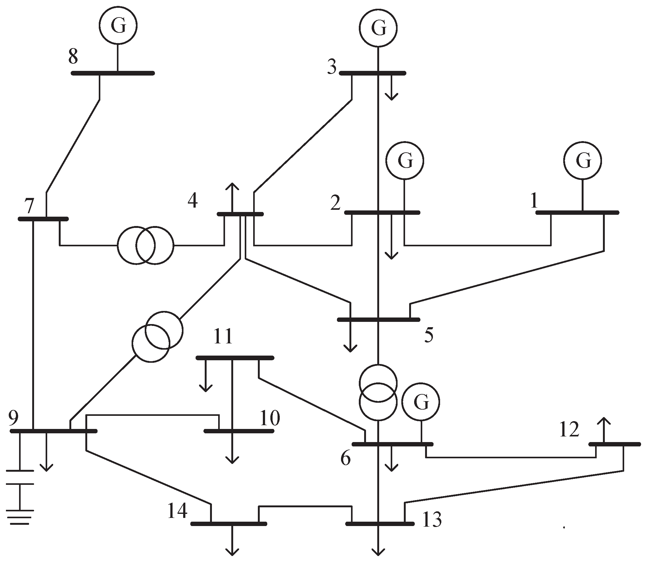
This paper introduces a detection approach that relies on state estimation. Considering the effectiveness of the method in real systems, the power standard IEEE-14-bus system shown in Figure 5 is used for MATLAB R2021b simulation. The active and reactive power of each bus are shown in the following

Table 3. Active and reactive power injections into system buses.

Bus	Generation	Generation	Load	Load
Number	Active (MW)	Reactive (Mvar)	Active (MW)	Reactive (Mvar)
1	2.3824	−0.1490	0.0000	0.0000
2	0.4000	0.4904	0.2170	0.1270
3	0.0000	0.2744	0.9420	0.1900
4	0.0000	0.0000	0.4780	−0.0390
5	0.0000	0.0000	0.0760	0.0160
6	0.0000	0.2960	0.1120	0.0750
7	0.0000	0.0000	0.0000	0.0000
8	0.0000	0.3092	0.0000	0.0000
9	0.0000	0.0000	0.2950	0.1660
10	0.0000	0.0000	0.0900	0.0580
11	0.0000	0.0000	0.0350	0.0180
12	0.0000	0.0000	0.0610	0.0160
13	0.0000	0.0000	0.1350	0.0580
14	0.0000	0.0000	0.1490	0.0500

. The data used in this paper come from MATPOWER trend calculation, which is used to obtain the bus voltage magnitude and phase-angle truth values, superimposed with zero-mean Gaussian white noise as the measurements. Furthermore, the estimation computations occur at one-minute intervals, which aligns with the anticipated average sampling frequency for utilities equipped with contemporary Energy management systems (EMS).

6.1. Comparison of Estimation Effects with WLS, EKF, and AIEKF

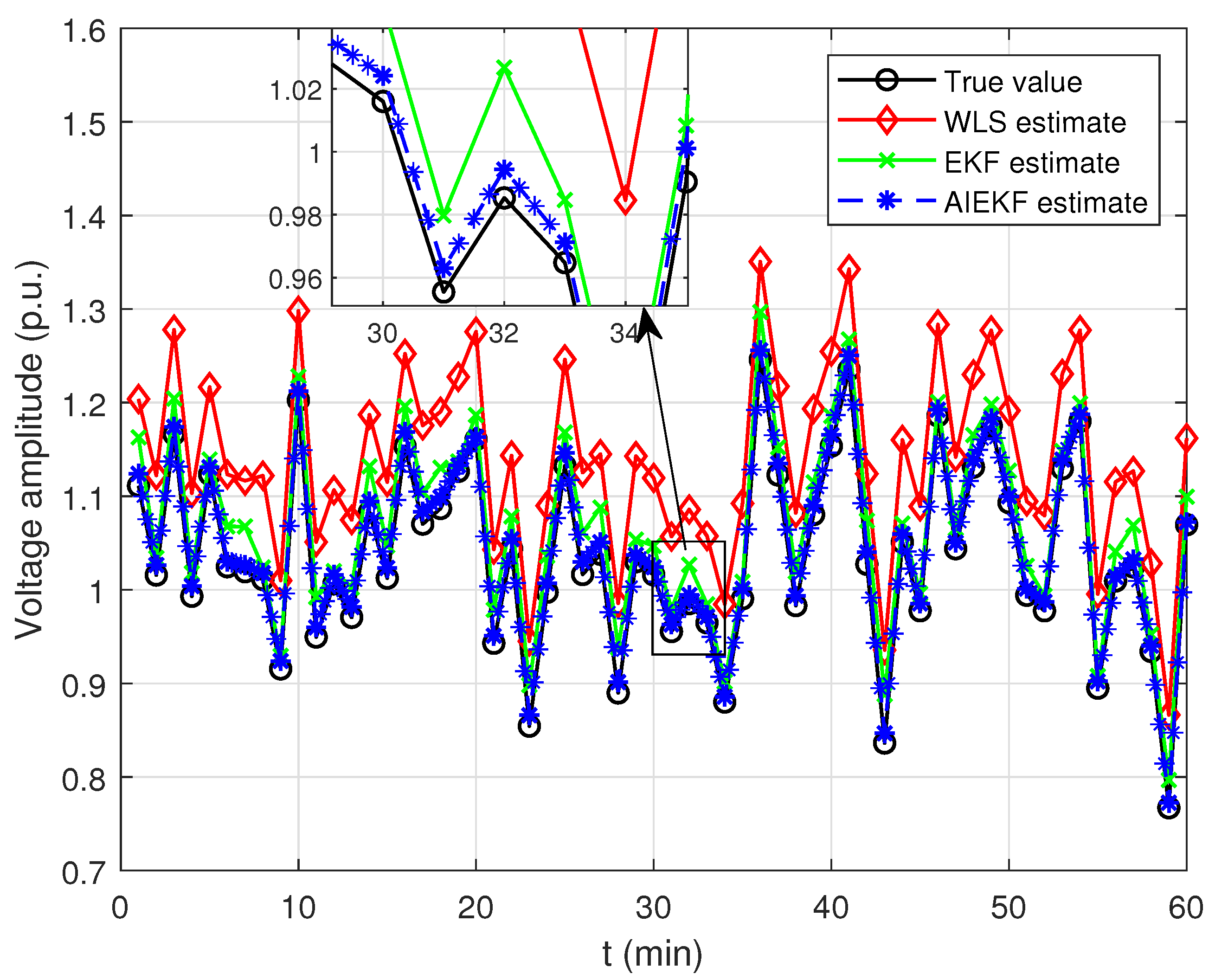
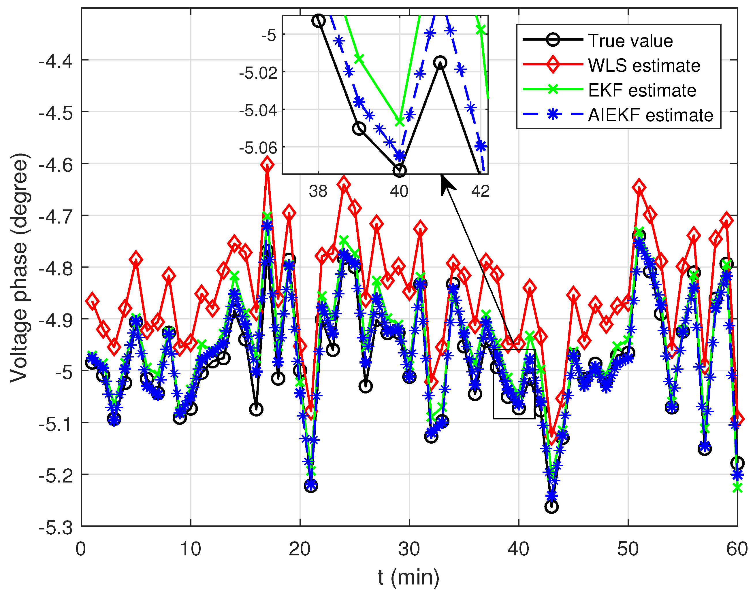
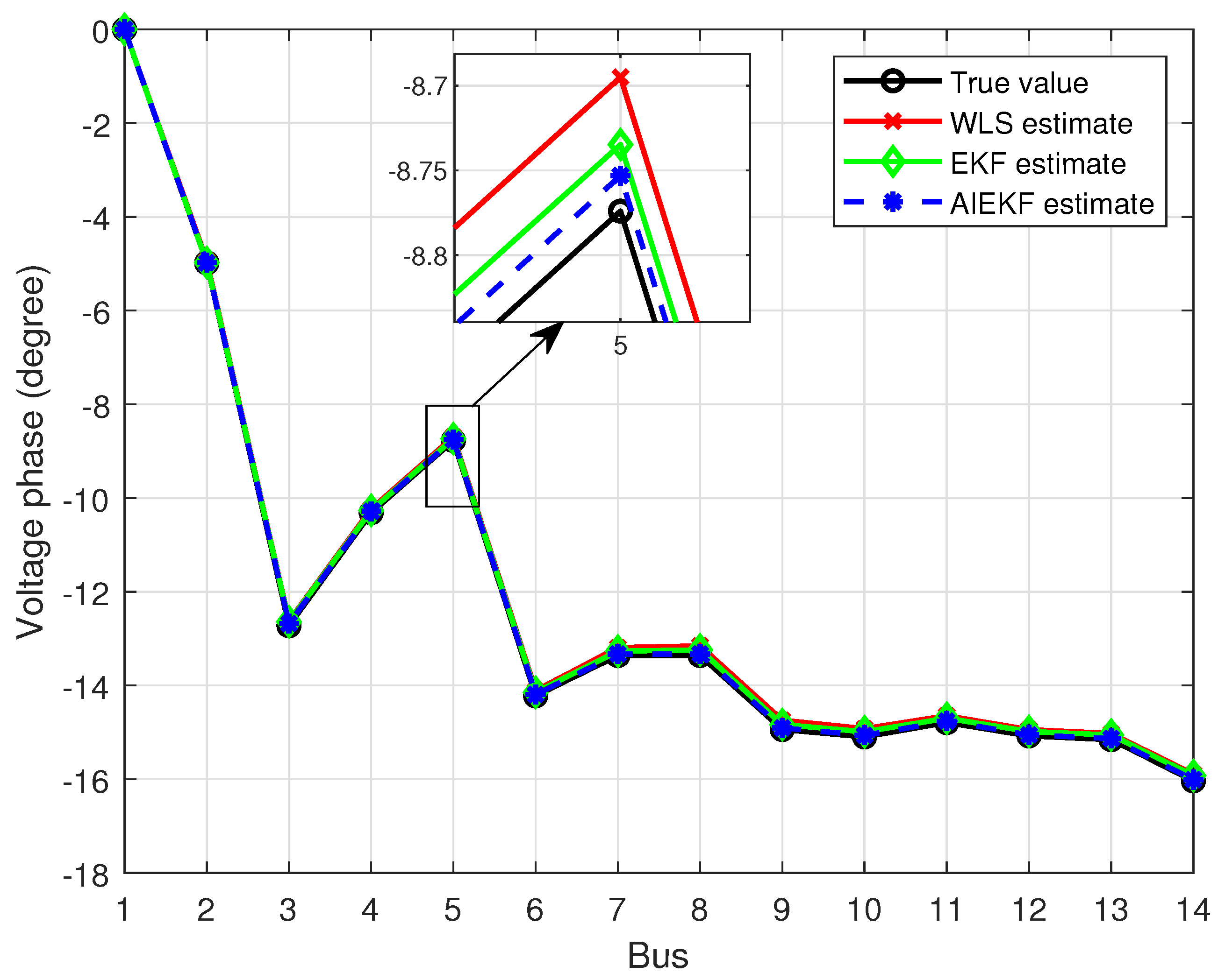
Next, the estimation effect of AIEKF proposed in this paper is compared with the standard WLS and EKF before injecting false data. As shown in Figure 6 and Figure 7, bus 11 was randomly selected to compare the estimation performance of the three algorithms in 60 min. It is clear to see from the figures that although the bus voltage and phase angle fluctuate up and down with time, the AIEKF achieves superior performance relative to WLS and EKF in state estimation. To further demonstrate the estimation capability of the proposed algorithm, the estimation results of the voltage amplitude and phase of each bus under the three algorithms after stabilization are shown in Figure 8 and Figure 9.

To validate the efficacy of the AIEKF algorithm introduced in this paper for state estimation, we use the root mean square error (RMSE) as a metric to assess the accuracy of the algorithm’s estimations. The RMSE calculation formula is provided below.

$$RMSE=\sqrt{\frac{1}{N}\sum _{i=1}^N{\left(x_i-{\widehat{x}}_i\right)}^2}$$

(36)

where $x_i$ is the ith component of the true value of the state variable, ${\widehat{x}}_i$ is the ith component of the estimation of the state variable, and N is the dimension of the state variable.

The RMSE performance metric is calculated in the IEEE-14-bus system, and the results are shown in

Table 4. Comparison of the RMSE of the three algorithms.

Algorithm	RMSE
WLS	0.0969
EKF	0.0616
AIEKF	0.0201

. As shown in Table 4, the RMSE of the AIEKF algorithm is the smallest of the three algorithms. Compared with WLS and EKF, the RMSE of the AIEKF algorithm decreases by 79% and 67%, respectively.

6.2. Estimation of the State Variable before and after FDIA

To assess the viability of the false data injection attack vector strategy, in this paper, we uses the IEEE-14-bus standard test system for simulation and analysis. An attack on a local subnetwork, e.g., an attack vector ($\mathit{a}$), is injected into each bus measurement value. Meanwhile, it is necessary to ensure that the internal power of the subnetwork is conserved and that the subnetwork boundary voltage and the transmission power between the subnetwork and the external network remain unchanged. The introduction of line blocking constraints leads to the response of the grid security analysis system so that the attacked measurement value ($\mathit{z}+\mathit{a}$) is a valid attack value. Under this condition, the attack vector ($\mathit{a}={[P_3,Q_3,P_{1-2},P_{2-3},P_{4-2},Q_{1-2},Q_{2-3},Q_{4-2}]}^T$) is selected as $\mathit{a}={\left[0.0020,-0.2029,0.0084,-0.0073,-0.0059,-0.4874,0.1329,-0.0723\right]}^T$, and the increment of the rest of $\mathit{z}$ is zero. 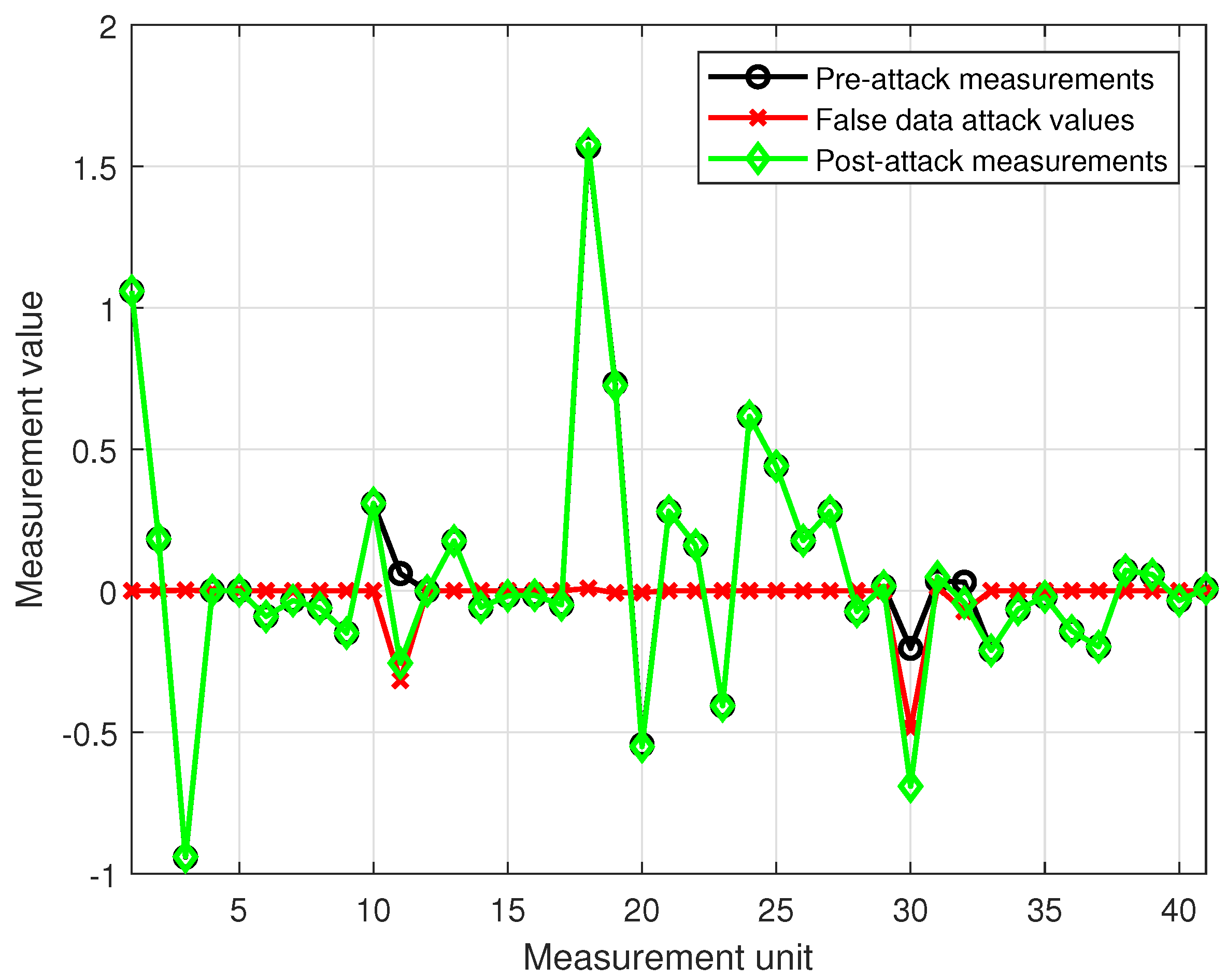Figure 10 shows the change in the measurement distribution of the system before and after the attack.

Once the measurements are tampered with, the state variable ($\mathit{x}$) changes. Assuming that the system is subjected to a false data injection attack at 75 min, bus 11 is selected to observe the change in bus voltage magnitude and phase angle before and after the false data injection attack occurs. State estimation of system buses using the AIEKF algorithm is performed to improve the stability and accuracy of the detection algorithm. The state estimation results of the two algorithms are shown in Figure 11 and Figure 12. As shown in the figures, in the first 75 min without an attack, AIEKF outperforms WLS in terms of estimation. The system is attacked by false data injection in the 75th minute, and the two algorithms converge to the state expectation at different moments. It is clear that AIEKF converges slowly and with small fluctuations, while WLS is affected by a sudden change in the measurements and converges quickly to the new state value.

6.3. Detection of FDIAs

Normal operation of the power information physics system produces a certain amount of error, but the residuals caused by measurement noise and system noise are often very small—much smaller than the threshold allowed for the detection of undesirable data errors—so that undesirable data can be prevented from interfering with the system. The values of $J\left(\widehat{x}\right)$ before and after an attack determined using weighted least squares are shown in Figure 13. Before the attack, the value of $J\left(\widehat{x}\right)$ is 4.5728. When the false data attack is injected into the system, the value of $J\left(\widehat{x}\right)$ is 4.7041. It is not difficult to find that the residual does not change much before and after an attack. The IEEE-14-bus system has a total of 41 measurements, the redundancy is $k=m-n=41-27=14$, and the significance level ($\alpha$) is 0.05. According to the statistical chi-square distribution table, the threshold of bad data detection is 23.685. The residual of the injected attack is within the threshold. However, the voltage amplitude and voltage phase are changed. The false data attack vector successfully achieves the attack.

This paper proposes a detection method based on the computation of the Euclidean distance between two points in the state space to detect FDIAs. Using Monte Carlo simulation with 1000 independent experiments, we can obtain the normal-case Euclidean distance distribution. The maximum value is taken as the detection threshold, i.e., $max\left\{d\left(1\right),\dots ,d\left(n\right),\dots \right\}=1.847$. The detection margin ($\mu$) is set to 0.03, and according to Equation (30), the detection threshold can be derived as ${\tau }_D=1.85$. After an attack, the Euclidean distance changes to 17.9586. 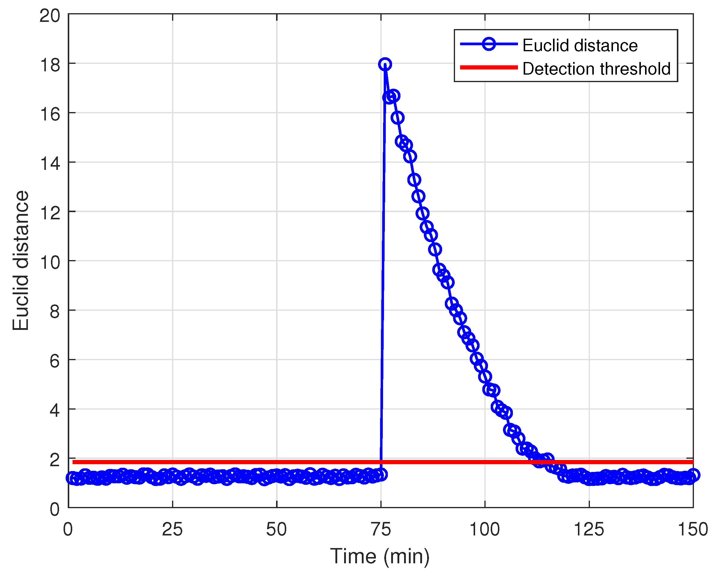Figure 14 shows the Euclidean distance distribution based on the two algorithms before and after an attack.

As can be seen from the figure, during the first 75 min, when the system is not under attack, the Euclidean distance between the state points stays within a certain range below the predefined detection threshold, which indicates that the system does not detect an attack according to the judgment conditions. When the system is attacked after the 75th minute, the two algorithms converge to the new state values at different moments. At this moment, the Euclidean distance of the voltage state estimate fluctuates considerably with the attack and exceeds the predefined detection threshold. Therefore, FDIAs can be detected, which triggers the attack alarm system.

7. Conclusions

In this research, we introduce an approach that combines weighted least squares with an adaptive interpolation extended Kalman filter to detect FDIAs in power systems. AIEKF effectively reduces the nonlinear errors associated with the extended Kalman filters, leading to enhanced accuracy in estimating the state of the power system. When a power system is subject to false data injection attacks, the state estimation weighted least squares statistic is characterized by a real-time nature, where changes in state variables are instantaneous, whereas adaptive interpolation extended Kalman filtering is characterized by hysteresis, and a change in state variables requires a process. Based on the difference between the two algorithms, the Euclidean distance is introduced as a metric for detecting whether the system is injected with false data or not. Additionally, the relevant detection threshold is obtained using Monte Carlo simulation. The experiments show that the method is effective in detecting false data injection attacks.

Subsequent research will consider the study of the localization of FDIAs and the development of a new joint estimation algorithm that can simultaneously achieve the detection and localization of false data injection attacks.