Short-Term Load Forecasting Using an LSTM Neural Network for a Grid Operator

Abstract

Electricity is crucial for daily life due to the number of activities that depend on it. To forecast future electric load, which changes over time and depends on various factors, grid operators (GOs) must create forecasting models for various time horizons with a high degree of accuracy because the results have a huge impact on their decision-making regarding, for example, the scheduling of power units to supply user consumption in the short or long term or the installation of new power plants. This has led to the exploration of multiple techniques like statistical models and Artificial Intelligence (AI), with Machine-Learning and Deep-Learning algorithms being the most popular in this latter field. This paper proposes a neural network-based model to forecast short-term load for a Colombian grid operator, considering a seven-day time horizon and using an LSTM recurrent neural network with historical load values from a region in Colombia and calendar features such as holidays and the current month corresponding to the target week. Unlike other LSTM implementations found in the literature, in this work, the LSTM cells read multiple load measurements at once, and the additional information (holidays and current month) is concatenated to the output of the LSTM. The result is used to feed a fully connected neural network to obtain the desired forecast. Due to social problems in the country, the load data presents a strange behavior, which, in principle, affects the prediction capacity of the model. Still, it is eventually able to adjust its forecasts accordingly. The regression metric MAPE measures the model performance, with the best predicted week having an error of 1.65% and the worst week having an error of 26.22%. Additionally, prediction intervals are estimated using bootstrapping.

1. Introduction

Electricity is delivered to consumers through a complex network, in which the first power plants generate it using technologies like gas turbines, hydro turbines, or solar photovoltaics, to name a few. It is carried over long distances using transmission lines and then commercialized, distributed, and finally used by customers (residential or industrial, for example) [1].

The amount of electricity end-use consumers consume varies and depends on multiple factors. For instance, there are some hours of the day when consumption tends to be higher than at other times (peak hours). Similarly, the consumption is different on weekdays, weekends, and holidays; in the latter two, the consumption is usually lower [2,3].

Likewise, population growth also plays an important role, especially in long-term load forecasting. These are just some examples of variables that have a specific impact on the variability of the electric load. However, there are more, such as weather conditions or the economic growth in a country [4,5,6].

Electric utilities need to anticipate, as accurately as possible, the future electric load because this information helps them meet demand and has an impact on their operating expenses and expansion planning (like the addition of new generating capacity) [7,8].

For grid operators, load forecasting represents a fundamental tool for decision-making regarding how generating resources will be managed in different time horizons (short-, medium-, and long-term) to deliver safe and reliable electricity to customers. Regarding the short-term, accurate forecasting results in the appropriate scheduling of power plants so that the generation is close to the actual demand for a specific period, which has technical and economic benefits from an operating and commercial point of view [7,8,9].

In addition, regulatory entities can fine a grid operator if its forecast differs considerably from the actual demand. For example, in Colombia, there is an entity named “Comisión de Regulación de Energía y Gas”, or CREG (https://creg.gov.co/, accessed on 2 October 2023) which states that daily differences between the forecasted and the actual load should be measured every hour. Economic sanctions will exist for those energy suppliers with a forecast percent error greater than a certain threshold. Furthermore, resolution 034 (2019) from CREG has highlighted that the companies must pay these penalties themselves, and they cannot charge the customers for that.

Consequently, the GOs must build forecasting models with low errors to avoid those economic sanctions. For this purpose, multiple techniques seek to solve the load-forecasting problem. Statistical models such as the Autoregressive Moving Average (ARMA) and its special cases like the Autoregressive (AR), Autoregressive Integrated Moving Average (ARIMA), and Seasonal Autoregressive Integrated Moving Average (SARIMA) models are some examples. Multiple regression models and Kalman filters have also been explored [10].

More recently, however, Machine-Learning (ML) and Deep-Learning (DL) algorithms have become relevant alternative tools to solve this problem. Neural Networks (NNs), for example, have been explored due to their capacity to deal with large amounts of data and extract relevant and complex features from it [11,12,13,14,15].

Nevertheless, regardless of the techniques or algorithms, the most crucial goal is to obtain an accurate forecast for appropriate power system management. Thus, the quality and reliability of the service could be better. This paper continues the exploration of NNs using an LSTM recurrent neural network to do a 7-day load forecast with a 1-h granularity for a department in Colombia.

The proposed methodology differs from previous works in that:

(i)

The load data used in this work is considerably affected by a national strike that took place in 2021. Since these social events are not unusual in countries like Colombia, it is important that the forecasting models used by GOs can somehow deal with these atypical behaviors by adjusting their output accordingly.

(ii)

It is common to use load lags to make predictions based on these past values. Since the number of LSTM cells matches the time lags in the input data, considering many lagged values could lead to complex models. In this work, the input data are structured so that the LSTM cells read multiple past values at once, reducing the number of required cells if the traditional approach was followed.

(iii)

When considering extra variables like weather data or calendar features, these are usually merged with the load data. In this work, the additional information is only considered once the LSTM has processed the entire historical data sequence. Specifically, it is concatenated to the LSTM’s output, and the resulting vector is used to feed a fully connected network to obtain the desired forecast.

(iv)

Prediction intervals are not usually reported along the forecasts made by DL-based models. In this work, they are estimated using bootstrapping, which means that as well as a single load value, the model additionally outputs an interval where this value could be for every predicted hour.

2. Literature Review

The authors in [7] used different ML algorithms to address the STLF problem in Panama, obtaining the best results with the extreme gradient boosting regressor (XGBoost). As inputs, the model employed data from multiple sources, such as historical load, weather, and calendar information. One of the advantages of implementing an XGBoost model is that it is possible to determine the feature importance from the input variables, which can facilitate its interpretation. However, the feature selection (FS) process plays a major role in determining which variables should be used to train an ML model. For this reason, the authors explored several FS techniques until they found the 13 most significant variables based on their contribution to the forecast. Among these, the load lags were the most important ones. Lagged load records from one, two, three, and four weeks ago were considered. The temperature information plays a critical role in STLF, according to their results. However, for forecasts beyond the dataset, it is necessary to use predicted temperature values, which can add more uncertainty to the load forecast. Moreover, this information is not always available in the required format.

On the other hand, DL algorithms have also attracted the community’s attention recently, with recurrent neural networks being generally the preferred choice in forecasting problems [16]. For example, ref. [11] studied and compared three Deep Neural Network (DNN) architectures: LSTM, GRU (Gated Recurrent Unit) and Drop-GRU, to solve the short-term power consumption forecasting problem and also prevent consumption peaks (by disconnecting load when necessary) for an area in a French city. The Drop-GRU was more efficient and performed better than the other two models on various time horizons. As inputs for the models, the authors only used power load data. Specifically, each topology reads a vector of n values: current and past power consumption values. In principle, the networks could predict consumption after 30 min, but through repetition and the right choice of hyperparameters, they could reach the desired time horizon. Although external factors were not considered in this work, the authors mentioned that including meteorological data and holiday information could improve their results. Adding a hyperparameter optimization stage could reduce the complexity of the proposed models and, in turn, reduce the execution time, which is a metric the authors monitored to evaluate the performance of the networks.

In contrast, ref. [12] proposed an optimized LSTM to make electricity consumption predictions in the short term (next 4 h) using Spanish electricity data. Again, no additional information was considered in the forecast. In this work, the LSTM was structured as a many-to-many problem. Since the data had a 10-minute frequency, the historical data window was set to 168 (1 day and 4 h), and the time horizon was limited to 24 (4 h). In this structure, the LSTM has a group of cells for the input data and another for the output. The authors tested their proposed DNN model against other DNN architectures, including a deep feed-forward neural network, a temporal fusion transformer, and some standard machine-learning methods. The LSTM model did better than the others because it could handle better how the data changed over time. A random search and the coronavirus optimization algorithm (CVOA) were used to find the best values of the hyperparameters for the LSTM, obtaining the lowest MAPE with the former.

In addition to historical consumption data, it is common to include information about variables that could affect this consumption so that DNN-based forecasting models can obtain better results. For example, ref. [6] forecasted the power consumption of two industrial buildings with different consumption patterns and considered a prediction horizon of 24 h. The authors used historical power load and weather data (temperature, humidity, sunlight, solar radiation, total cloud cover, wind speed, wind direction, humidity, and vapor pressure). Four DNN-based univariate and multivariate forecasting models were proposed by selecting the amount of data used to feed them. The best performance was obtained when using a Multi-Layer Perceptron (MLP), RNN, and LSTM and considering historical consumption data from one or two years ago and no weather data. The addition of weather variables also showed promising results, but only when those that affected the power consumption were chosen, making their selection a critical step when this additional information is considered. The authors also proposed a method to correct the prediction error when the power consumption changes quickly.

Another example is [8], where Feed-forward Deep Neural Network (FF-DNN) and Recurrent Deep Neural Network (R-DNN) models were built to address the short-term load-forecasting problem using load data from six states in New England, USA. The authors not only used time domain features but also time-frequency features. Specifically, they considered time domain features like weather, time, holidays, lagged load, and load distribution. Regarding the frequency domain, a Fourier Analysis was performed to identify dominant frequencies in the load data. A high pass filter was designed to filter out low frequencies, and the remaining signals were converted back to the time domain. The authors improved their results when using both sets of features. In this work, the recurrent network outperformed the feed-forward network.

In [14], the authors compared the performance of an LSTM and traditional methods, such as ARMA, SARIMA, and ARMAX, to address the STLF problem for different prediction horizons. As well as historical load data, temperature data were also used to feed the models. In contrast to other works, prediction intervals were included, considering a 95% confidence interval. However, their computation was not detailed (specifically for the LSTM implementation). Based on MAPE results, the implemented LSTM showed a better performance for prediction horizons of 24 and 48 h. However, for 7 and 30 days, the traditional methods outperformed the LSTM.

The authors in [17] also implemented an LSTM recurrent neural network to address the load-forecasting problem for different time horizons using data from a region in France. First, several ML algorithms were trained with historical load values, weather information, and calendar features. The best one was chosen as a benchmark for the DL-based model. By exploring the importance of the input features, they concluded that the lags had the highest relevance and then used a genetic algorithm to select the most relevant ones, which were the inputs for the LSTM implementation. This step was taken because using many lagged values increases the dimensionality of the problem and the complexity of the network. Ultimately, the recurrent network showed a lower forecast error than the benchmark ML model (Extra Trees Regressor).

Although forecasting models are often built using a single network, it is possible to combine multiple networks. For example, ref. [13] proposed a hybrid model based on empirical mode decomposition (EMD), a one-dimensional convolutional neural network (1D-CNN), a temporal convolutional network (TCN), a self-attention mechanism (SAM), and an LSTM. The authors considered temperature, day types, and seasons as external factors affecting the changes in energy use. The load data were decomposed into several sub-series, and those with a significant correlation with the original time series were selected. The CNN, TCN, and SAM were used together to improve the feature extraction process, and the LSTM was the model used as a predictor.

Another example of a forecasting hybrid model is presented in [18], where the authors utilized several DL algorithms to forecast household power consumption in the near term using historical consumption data, including multiple electrical quantities, such as voltage and global active and reactive power from a home in France, and calendar features. Residential power consumption data are a challenge because, at that scale, the behavior of the residents also plays an important role in the consumption patterns and must, therefore, be taken into account. The best-performing model was a hybrid neural network, CNN-LSTM. The CNN was used for feature extraction between variables affecting energy consumption (spatial correlation) and noise removal. Then, the outputs of the last convolutional layer were passed to an LSTM, which handled the temporal nature of the data. Finally, the last output of the recurrent layers passed through a fully connected (FC) layer to generate the predicted consumption values. Regardless of the type of network, it is common to have an FC layer at the end of the model with the same number of neurons according to the considered time horizon and forecast resolution.

In [15], a hybrid deep-learning model is also implemented using CNN and LSTM networks to solve the STLF problem. For comparison, some ML-based models were implemented as well. Regarding the hybrid model, as before, the CNN extracted input data features while the LSTM handled the long-term dependency within the input data. However, in this opportunity, the networks were not connected. Instead, they worked independently in parallel paths. Then, the outputs from both paths were concatenated and passed first through another LSTM layer and then through a fully connected network to obtain the desired forecast. The authors did not consider exogenous variables. The proposed hybrid model outperformed the other models on two different datasets.

Also, ref. [19] proposed a flexible power consumption forecasting model for different short time horizons with minor changes in the preprocessing phase and the ability to work in more than one geographical place. The model was built using a set of four neural networks: CNN, LSTM, CNN-LSTM, and MLP. Each network had a different performance under specific conditions, and a weight function dynamically gave them a value corresponding to their importance in the final prediction. The goal was to select the best networks for a particular scenario automatically. The model was tested with load consumption data from Panama and a French island. Only historical data were considered in the first case, while the second case also considered weather and holiday information.

The remainder of this paper is organized as follows: Section 3 provides details about the input dataset, preprocessing steps, chosen DNN architecture, and selection of additional features to feed the forecasting model. Section 4 describes how the short-term load-forecasting problem was addressed with an LSTM to make predictions on the desired time horizon and presents the results and analysis of the applied methodology and the estimation of prediction intervals. A performance comparison between a benchmark model and the proposed model is presented as well. Finally, Section 5 has the conclusions derived from this research.

3. Data Description and Preprocessing

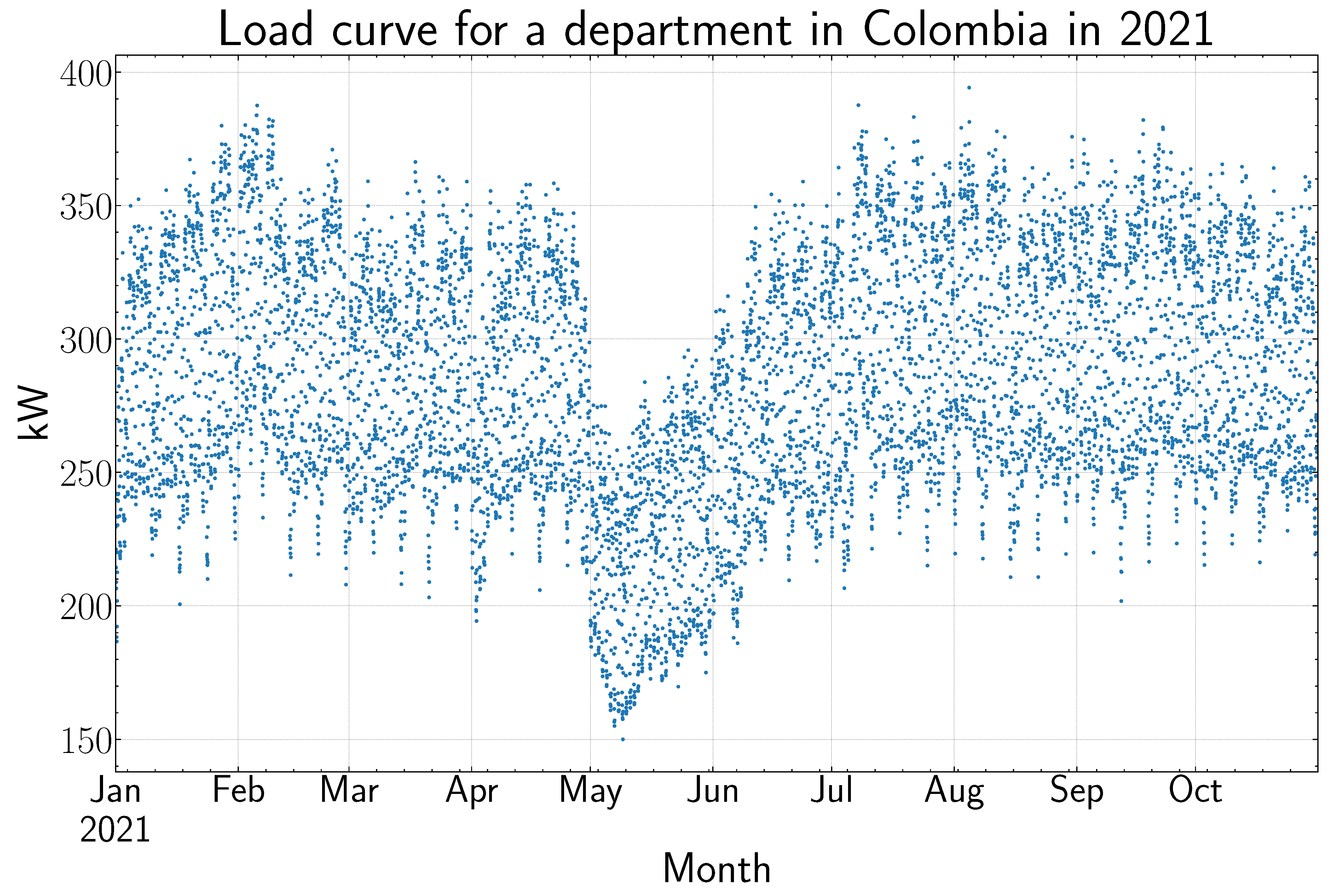
The database contains load information from a department in Colombia ranging from 6 June 2009 to 31 October 2021 with a resolution of one hour, and it is partially preprocessed (however, it has some outliers and missing values). In the last year, a national strike took place in the country, which significantly affected the behavior of the load curve for about three months (May–July), as can be seen in Figure 1. This dataset was provided by a Colombian GO, and it is not publicly available.

There is no data for 2472 h (corresponding to 103 days). These missing load values are only found in the early years. The interquartile range $iqr$ was computed to identify outliers, which is the difference between the third and first quartiles ($q3-q1$). Then, values greater than $q3+1.5·iqr$ and lower than $q1-1.5·iqr$ were removed. In total, 32 load values were marked as outliers. These values correspond to hours in years before 2020, which means that despite the strike’s impact in 2021, the corresponding load values during the affected period are not statistically considered outliers.

The next step is to input the missing values (2504 values in total). Each missing value is replaced with the median of the values having the same temporal characteristics in terms of year, day type, and hour. For example, if one of the missing values is the load on Friday 10th 2017 at 8:00 a.m., then it is replaced by the median of the load values on Fridays in 2017 at 8:00 a.m. After doing this, the result is a time series without missing dates and outliers.

A descriptive analysis is performed to find relevant characteristics of the load curve that the DNN model can use. Figure 2 and Figure 3 show how the load values vary as a function of the time of day and day type, respectively. As we mentioned before, people tend to consume more electrical energy on weekdays in contrast to what they do on weekends and holidays (especially on Sundays), and from Monday to Friday, the daily median load values are similar. Also, consumers are more active in the afternoon-evening than in the morning, and there is a peak in consumption between 6 and 9 in the evening, regardless of the day type.

It is also interesting to see how the current load data relate to their previous values. For this purpose, the Autocorrelation Function (ACF) is computed, and it appears in Figure 4, where the seasonality in the time series is evident (especially weekly). Only 336 lags (two weeks) are plotted for clarity, and two black dashed lines highlight the lags corresponding to one and two weeks, respectively. This behavior is found even considering a higher number of lags.

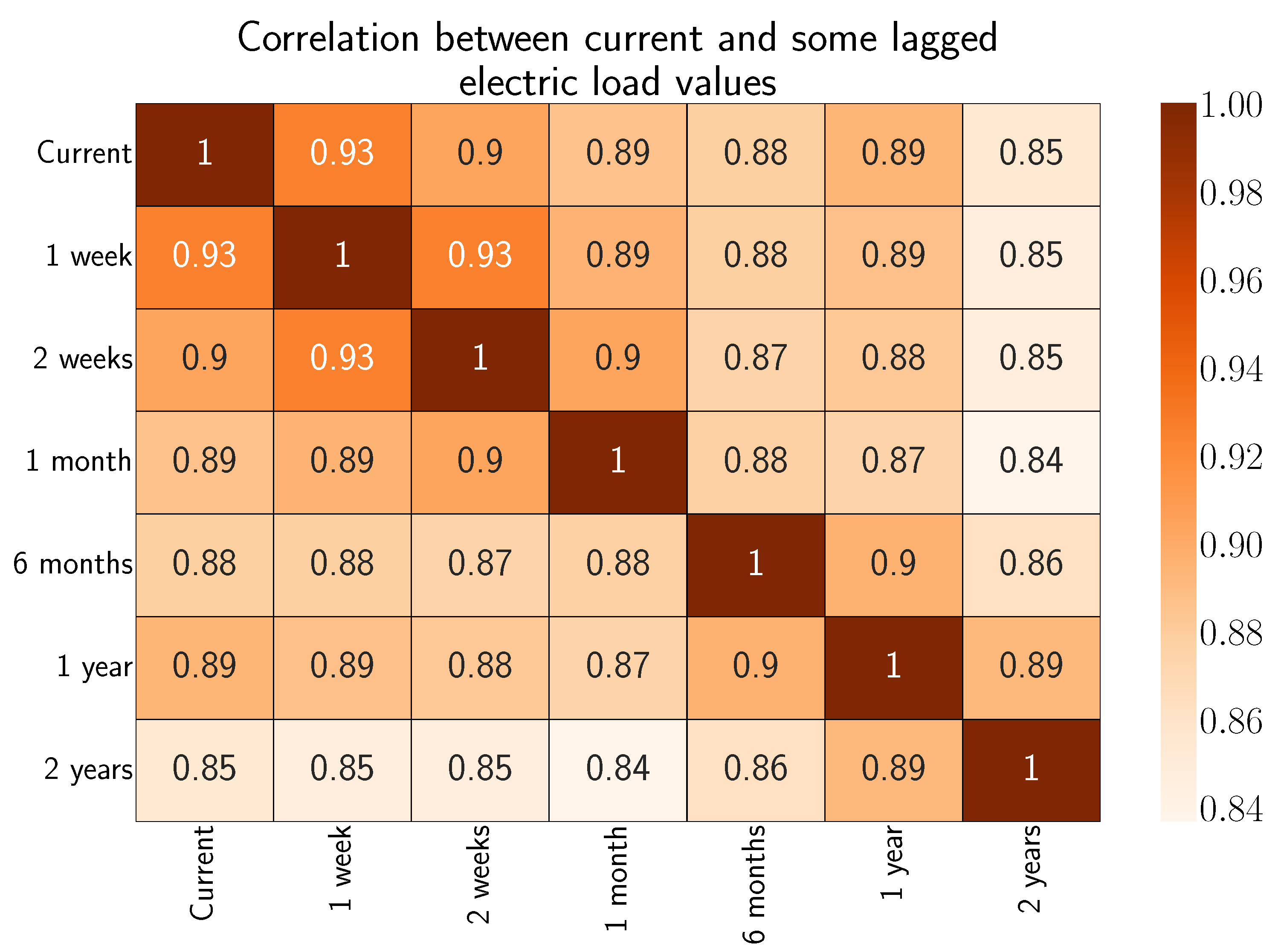
A correlation matrix is employed to observe the impact of older load values on current ones. Figure 5 shows a strong correlation even with 1-year-lagged values, which agrees with what was found previously in the ACF plot.

Finally, an XGBoost is implemented as it is possible to visualize the importance of the features used by the model in the prediction of one variable, and this information, along with the previous analysis using box plots, ACF plots, and correlation matrix, can help to select the input variables for the DL model. In this case, the XGB is trained using almost all the data except the last two weeks used for testing. Figure 6 reveals that the most important feature is the load value from 168 h (or one week) ago, then a variable indicating which days in the target week are holidays, and in third place the load value from 8736 h (or one year) ago.

The final decision is to feed the LSTM with the information about load from the last year (which, in fact, also includes many of the most important lags found before) to predict the load for one week with a one-hour resolution. Also, the network considers which days in the target week are holidays and which month this week is in. This last calendar feature is included because many months have unique characteristics that could affect the behavior of the end-use consumers (Holy Week, Christmas celebrations, or vacation periods).

The chosen DNN model is an LSTM. This type of recurrent neural network has been a typical DL architecture used to solve the short load-forecasting problem [8,11,13,14,15,17,18,19]. It is important to define the way the LSTM will process the data. First, the load values are all divided by the smallest integer greater than the maximum load value in the database to keep the numbers between 0 and 1. Then, the time series is broken into X and y pairs to turn the problem into a supervised learning one so that the model can learn a mapping between them. Here, X are the inputs, and y are the corresponding labels. For this purpose, the sliding window technique creates samples with the required structure. For example, the first sample corresponds to the hourly load information from the first 52 weeks (one year) and is organized from oldest to newest. The associated target is the hourly load data for the following week. All the weeks are considered to start on Saturday and finish on Friday. This convention is followed because the deadline for grid operators in Colombia to report their forecasts for a week is Friday from the previous week. It is explained in more detail in resolution 025 (1995) from CREG.

4. Results and Analysis

4.1. Deep Neural Network—DNN

One of the advantages of an LSTM over a simple RNN is its capacity to learn long-term dependencies, which is a weak point in the traditional recurrent neural network because of the vanishing gradient problem [20]. An LSTM is a group of interconnected cells that process the values from an input sequence. Each LSTM cell has a series of gates working together to modify the network’s long-term memory and determine what information should pass to the next cell. Every LSTM cell produces an output, but generally, the output of the last LSTM cell is used for further processing since the entire sequence has been read at this point.

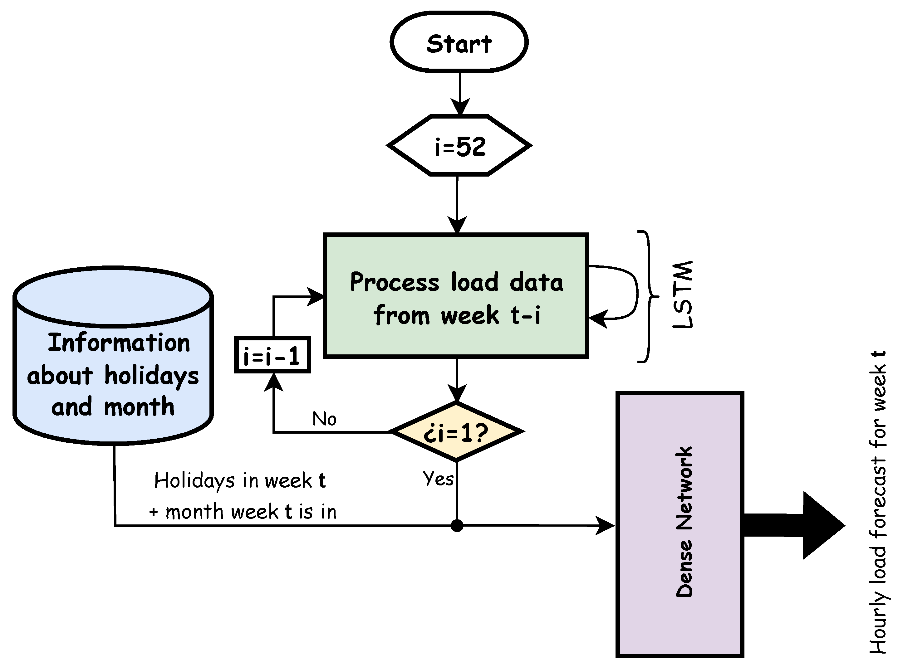
Figure 7 summarizes the way the forecasting model works. In the proposed method, every input sequence is 52 weeks long, and the elements of the sequences are the hourly load data from each week (168 values). Therefore, for every input sequence, the LSTM reads the load values from the oldest week $t-52$ to the most recent week $t-1$.

The output of the LSTM, obtained after reading the entire sequence, is concatenated into two arrays. The first one is a $1\times 7$ array directly related to the seven days of the week and following the convention explained before about the first and last days of the week. This array is filled with zeros except at indices where the associated day is a holiday. The second array is $1\times 4$ long and encodes the month the forecasted week is in (using Gray code from 0001 for January to 1010 for December). At this point, the resulting array is processed by a fully connected network that outputs 168 values corresponding to the load for every hour in the target week t.

4.2. Processing Data

The windowing process generated 595 sequences, split into training/validation (80%, i.e., 476 sequences) and test (20%, i.e., 119 sequences). For the validation, a common technique known as k-fold cross-validation is used, where k identical models (same configuration of hyperparameters) are trained and validated with similar training sets but different validation sets. Figure 8 illustrates the process.

The overall validation performance can then be computed as the average of the individual validation performances. To compute the training performance, a new model can be created (using the same configuration of hyperparameters), but this time using the entire training/validation set to train it [20]. In this work, the regression metric MAPE will be used to measure the forecast error:

$$\mathit{MAPE}=\frac{1}{N}\sum _{i=1}^N\left|\frac{x_i-y_i}{x_i}\right|,$$

(1)

where $x_i$ and $y_i$ are the ground truth and predicted values, respectively, and N is the total number of samples.

On the other hand, hyperparameter search is performed using the random method, which tests multiple randomly selected combinations from a defined grid of hyperparameters. Wandb (Weights and Biases, https://wandb.ai/site, accessed on 3 October 2023) tool application is used for this purpose.

The LSTM’s training, validation, and testing performances are shown in

Table 1. Performance of the LSTM.

MAPETRAIN [%]	MAPECV [%]	ID	MAPETEST [%]
3.25	3.65	0.039	3.73

. The overall RMSE on the test set was also computed since it is a common metric used to evaluate forecasting models, yielding a value of 14.39 kW. There is also a measure of the variation of the validation performance between the different folds known as Index of Dispersion (ID). The best configuration of hyperparameters found by wandb is listed in

Table 2. Best hyperparameters found with Wandb.

Hyperparameter	Value
Batch size	32
Number of LSTM layers	1
LSTM units	128
Number of dense layers	1
Activation (dense layer)	tanh
Dense units	64
Number of epochs	350

. In total, 30 combinations were tested. The dense layer configuration corresponds to a layer before the actual output layer, which is fixed and has 168 neurons and a linear activation function. Regarding the optimizer, Adam was chosen and used with its default configuration.

The LSTM performed better on the training set than the test set, which, at first glance, could be considered an indicator of overfitting. However, it is important to highlight that the test set covers recent years of data. Therefore, there were a few weeks corresponding to the national strike where the model probably had more problems forecasting the load values accurately, which could have led to significantly high errors and eventually affected the overall performance on the test.

That behavior is presented in Figure 9, where the worst forecasted week corresponds indeed to the first week (from Saturday to Friday, following the convention explained before) after the start of the strike (28 April 2021). The lowest and highest MAPE on test were 1.65% and 26.22%, respectively. Regarding the RMSE on the test set, the lowest and highest values were 5.92 kW and 62.51 kW, respectively.

It is also interesting to see how the model performs during the weeks where the impact of the national strike on the load curve had a significant effect (see Figure 1). The hourly load values forecasted from 1–7 May are above the actual values, which makes sense because the LSTM does not have a way to anticipate such abrupt change, and this can explain the overestimation of the load. However, in the following weeks, when the network has some knowledge about what is happening, the forecast errors start to take lower values. On the other hand, the first week after the load curve completely recovers from the effect of the national strike (from 3–9 July), there is an underestimation of the load because, again, the LSTM cannot anticipate this change. Afterward, the error for the following weeks lies below 4%. The described behavior is shown in Figure 10, where the MAPE for the first week after the effect of the strike has been circled in red.

The additional information given to the LSTM (holiday and month) positively affected its results, as seen in

Table 3. MAPE on the test set (119 weeks) changing the additional data included in the DNN model.

	MAPETEST [%]
ineLoad + holidays + month	3.73
Load + holidays	4.07
Load + month	4.43
Only Load	4.34

. This time, three new LSTM models were created and trained using the same configuration of hyperparameters shown in Table 2, providing additional information to make the forecast. The first row corresponds to the MAPE on the test with the original model. The second row corresponds to a model that only considers holiday information. The third row corresponds to a model with only monthly information, and the last row corresponds to a model with no additional information.

To further observe the effect of the national strike on the load curve, an additional experiment where the end of the time series was set to be before the strike was considered. In this scenario, the MAPEs in training data, cross-validation (CV), and testing data were 3.44%, 3.51%, and 3.57%, respectively, while the index of dispersion (ID) was 0.038. There is a slight performance improvement, which was expected since the atypical behavior of the load curve due to the strike was not considered. The reported performance was found with an LSTM having the following hyperparameters: batch size-64, number of LSTM layers-1, LSTM units-64, no dense layers, and number of epochs-500. The total number of learnable parameters was 72416, which is less than the parameters of the LSTM considering the effect of the strike (171944). Regarding the data splitting, an 80/20 approach was also used (80% for training/validation and the remaining 20% for testing).

4.3. Comparison between Implemented LSTM and Benchmark Model

ML-based models are popular choices for time series forecasting problems [7,12,15,17]. Therefore, in this work, an XGB was considered a benchmark model to compare its performance on test data against the proposed DL-based model. For the XGB, the preprocessing steps and data splitting explained before were applied. One of the main differences between both models is the way the data are fed into them: for the XGB, the train, validation, and test sets are all pandas data frames. Each data frame has 55 columns:

• One column corresponds to the target (hourly electric load).
• Two columns correspond to calendar features (one for holidays and another for months).
• The remaining 52 columns correspond to lagged values (one week ago, two weeks ago, …, 52 weeks ago).

Overall, the performance decreased in terms of MAPE on the test set where 119 weeks were considered (see

Table 4. Comparison in terms of MAPE between the proposed model and an XGB model on test.

Model	MAPE [%]	RMSE [kW]
LSTM	3.73	14.39
XGB	4.65	18.04

). Also, the performance was poorer during the weeks affected by the strike in 2021. The evolution of MAPE for the weeks during the national strike is presented in Figure 11.

One of the reasons that could explain the higher MAPE is the fact that in contrast to the LSTM, the XGB model is considering only 52 lags corresponding to the load values on the same day at the same time in previous weeks with respect to the target. For example, to forecast the power load on Monday at 6:00 a.m. in the week t, the XGB only considers the power load on that day at that time from previous weeks ($t-1,t-2,\dots ,t-52$). The LSTM, on the other hand, would take into account the whole history from the past year (i.e., what happened in the previous 8736 h), which gives the network more context about the recent behavior of the load curve. To check this, a new XGB model was built, but this time, all the 8736 lagged values were considered. With this new implementation, the overall MAPE was 2.13% (and the RMSE was 8.41 kW), outperforming the proposed LSTM (even during the strike period). However, the training was computationally more expensive in terms of memory consumption and execution time due to the complexity of the input data frames. The LSTM provides more flexibility regarding the way the input data are structured to feed it, and using the hyperparameters presented in Table 2, its training took almost 2 min (including the cross-validation step). So, it is a trade-off between performance and computational complexity that should be resolved according to the OG’s requirements and needs.

4.4. Prediction Intervals

There is no standard method to compute the prediction interval for a forecast made by a neural network. However, one possible approach is to use a statistical procedure known as bootstrapping, in which a single dataset is resampled many times (typically 1000 or more), and from these new samples, some statistics about the original set can be estimated.

In the context of this work, the procedure can be applied by building and training a thousand LSTM models with the same configuration of hyperparameters shown in Table 2. Then, each model is used to forecast the hourly load for the 119 weeks on the test set, which results in 1000 values for every hour of every week. The forecast can then be defined as the average of such values. Regarding the prediction intervals, the upper and lower limits can be computed as the percentiles $p=2.5$ and $p=97.5$, respectively (considering a 95% confidence interval). Figure 12 summarizes the described procedure to compute the prediction intervals, and Figure 13 shows the weeks with the lowest and highest MAPE and RMSE presented before, but where the corresponding prediction intervals have been included and represented by a green-shaded area. Regarding the plot at the bottom, the forecast and corresponding prediction interval could be interpreted as the expected load if the strike had not occurred. On the other hand, the forecast error for the best and worst forecasted weeks decreased a little using the average of the load values forecasted by the 1000 models; in fact, the MAPE on the test is now 3.64%. The lowest and highest MAPE on test were 1.42% and 26.15%, respectively, in this case. Regarding the RMSE on the test set, the lowest and highest values were 5.04 kW and 61.75 kW, respectively.

5. Conclusions

The deep neural network architecture implemented in this work was a vanilla LSTM using the Keras framework. The results are similar to the ones reported in the reviewed literature for the STLF problem. ML-based models have proved to be a powerful tool in forecasting problems, and one of their advantages over DL-based models is that they are not entirely a black box. For example, algorithms like XGB show the importance of the input features used to forecast a variable. However, these models generally require a more exhaustive feature extraction step. In contrast, in this work, the information selected as inputs for the LSTM was extracted mainly from an ACF plot and a correlation matrix, letting the network decide about the most crucial information to make the forecast internally.

As observed, adding additional information like calendar features to the forecasting model positively impacts the results. Based on the MAPE values presented in Table 3, the information about which days in the target week are holidays seems to be the most relevant for the model taking into account that, although the MAPE on test increased, this increment was lower in comparison to the other scenarios where no information about holidays was included.

It is essential to highlight that grid operators should take into account, as well as the forecast itself, that sometimes unexpected events with a significant impact on the load curve can occur, and this will make the forecasted values distant from the actual ones (leading to a high forecast error) because the forecasting model cannot anticipate such events. Therefore, it is necessary to have a plan to overcome this issue so that they can schedule the power units accordingly.

One of the main applications of STLF is the scheduling of the power units that will operate in the short term (e.g., next week) to supply the users’ consumption. Since there is no perfect forecasting model, the predictions will always have an associated error. This forces the GOs to buy energy in the market if, for example, the actual consumption is higher than expected. Also, if the differences are significant, they can lead to fines. Estimating a range of values where the consumption could be for every predicted hour could help GOs anticipate such situations and make them act accordingly.

Although the goal of this work is not to outperform existing forecasting models, the results are promising, especially taking into account the abnormality found in the dataset (due to the national strike) and the fact that as additional information, only calendar features were considered, in contrast to other works found in the reviewed literature where the authors had access to other variables affecting the power consumption. Also, the methodology included a different approach for implementing an LSTM and estimating prediction intervals, which are not commonly reported.