Research on Risk Measurement of China’s Carbon Trading Market

Abstract

In today’s environmentally conscious world, carbon trading has emerged as a widely accepted economic instrument to mitigate the externalities resulting from deteriorating environmental problems. Consequently, the use of market-based mechanisms to address environmental issues has reached a global consensus. Many countries are implementing progressive steps by establishing carbon markets to promote low-carbon development and meet their carbon reduction targets. However, the inherent risks in carbon trading markets may hamper the formation of a reasonable carbon price signal, leading to inadequate stimulation of low-carbon technology investments and potential failure to achieve national emission reduction goals. Therefore, managing the risks associated with carbon trading markets is crucial. This study focuses on measuring the risk of China’s carbon market, with the primary aim of exploring carbon price fluctuation patterns and precisely measuring market risks. The risks associated with China’s carbon market are quantified and analyzed using the exponential generalized autoregressive conditional heteroskedasticity (EGARCH) model, extreme value theory (EVT), and the value at risk (VaR) method. Results show that (1) the effect of external shocks on each carbon market is asymmetrical, and positive shocks exert considerable leverage effects on carbon price fluctuations. (2) EVT can be used to effectively fit the risks in the carbon markets. The risks of each carbon market show different characteristics. The risk of Hubei and Guangdong carbon markets is relatively small, and the dynamic VaR is nearly ±0.2. (3) Compared with the performance of the Chinese carbon market, the performance of the European Union Emission Trading Scheme is more stable, and its dynamic VaR for most of the period is within ±0.1, which is considerably lower than the VaR of other Chinese carbon markets. This study also proposes suitable policy implications to ensure the healthy and sustainable development of China’s carbon market.

1. Introduction

In recent years, humanity has faced serious threats, including rising sea levels, frequent haze occurrences, and global warming, caused by climate change. These changes pose great risks to our living environment. The development of a low-carbon economy to address the ecological and environmental issues caused by climate change and ensure a sustainable habitat for humanity has reached a global consensus. With the rapid development of China’s economy and society in recent years, the country’s greenhouse gas emissions have also been steadily increasing. China is the world’s largest emitter of carbon dioxide, with its total emissions reaching 11.48 billion tons in 2022 [1], covering about one-third of the world’s carbon emissions. Despite China’s commitment to achieve peak carbon emissions by 2030 and carbon neutrality by 2060, as announced during the 75th United Nations General Assembly in 2020, the sheer scale of carbon emissions and the urgency of the situation present numerous challenges to achieving the two carbon goals. Carbon markets are effective, cost-efficient solutions to address climate issues [2]. They work by internalizing the external costs of emissions, thus promoting low-carbon transformation and technological innovation in businesses [3]. In 2015, China established carbon trading pilot markets in nine provincial-level regions, and in 2021, the national carbon market officially began operating. This carbon market is viewed as a crucial tool in achieving China’s climate goals by incentivizing emission reductions and fostering a transition to a low-carbon economy.

Currently, China’s carbon market has promising development prospects, but in comparison with mature carbon markets, such as the European Union Emissions Trading System (EU-ETS), it is still in a continuous improvement phase [4,5]. It poses complex risks for its participants because of policy uncertainties, supply–demand dynamics, and the influence of external factors has resulted in sharp fluctuations in the carbon price [6]. In the case of the EU-ETS, during its first and second phases, carbon prices faced considerable shocks, resulting in sustained price fluctuations and a depressed market [7], which had severe adverse effects on the effectiveness of the carbon market and participating companies. At present, China’s carbon market is in a highly uncertain phase and characterized by substantial price fluctuations and relatively low prices [8,9]. Therefore, effectively assessing the volatility risks in the Chinese carbon market is essential [10,11]. Such an assessment can guide market regulators in formulating effective carbon market control policies to mitigate the occurrence of extreme risks, which in turn can help participating companies effectively manage their exposure to risks and prevent serious losses.

In carbon markets, risks are closely associated with fluctuations in carbon prices. The volatility of carbon prices effectively reflects market conditions, and the price fluctuations that occur during the trading process are considered normal [12]. However, excessively low and high price fluctuations can lead to upward and downward risks in carbon prices, highlighting the importance of maintaining carbon price fluctuations within a normal range. Ren et al. (2017) [13] observed that carbon price fluctuations in the Shenzhen carbon market exhibit long-term memory. Fu et al. (2020) [14] employed an ARMA-EGARCH-SGD model to investigate the effect of information on return volatility and found that the influence of information is asymmetric. Furthermore, they noted that except for the carbon markets in Hubei and Chongqing, other pilot carbon markets are more affected by positive shocks than by negative ones. Zhang et al. (2020) [9] used a generalized autoregressive conditional heteroskedasticity (GARCH) model to analyze the price fluctuations in the Shenzhen carbon market. Their research indicated that the volatility of carbon price returns in the Shenzhen carbon market is gradually stabilizing. However, starting in 2018, factors, such as economic downturn and insufficient market information, led to an increase in the amplitude of carbon price fluctuations. Lyu et al. (2020) [15] conducted empirical analyses on China’s carbon trading pilot markets using the Markov chain Monte Carlo–stochastic volatility model and the wavelet multiresolution model. They discovered that carbon prices in Hubei, Shanghai, and Shenzhen exhibit clustered volatility, with large price fluctuations and inadequate stability. Liu et al. (2020) [16] employed the stochastic volatility with leverage model to describe the price fluctuations in five carbon markets in China. Their findings indicated considerable differences in carbon price fluctuations in these markets. Specifically, Shenzhen, Guangdong, Shanghai, and Beijing exhibited positive leverage effects, and Hubei displayed a negative leverage effect. Since financial time series may contain trend components that can impact the analytical results [17], because the mechanism for generating the trend component differs from the fluctuation mechanism of the cyclical component, and the trend component has an impact on the estimation of the period component [18], the authors utilized a trend-cycle decomposition model to separate these components and reveal their underlying temporal characteristics and driving forces. In this regard, the Hodrick–Prescott (HP) filter, as a nonstationary signal processing method, is widely applied in market price volatility analyses. Liu et al. (2018) [19] employed the HP filter method to analyze the price fluctuations, trends, and patterns in the Xinjiang red date market. Their research revealed a remarkable downward trend in red date market prices, pronounced seasonal effects on price fluctuations, evident cyclical price changes, a gradual narrowing of price fluctuations, and an increase in the frequency of price fluctuations. Similarly, Jia et al. (2018) [20] used the HP filter method to analyze price fluctuation characteristics in the Chinese barley market. Liu et al. (2023) [21] removed the long-term trend in oil prices using the HP technique to reflect the fluctuation pattern. Their results indicated notable seasonality and cyclical patterns in Chinese barley prices. Moreover, Chinese barley prices exhibit an overall decreasing trend, remarkable volatility clustering, and asymmetry features.

Quantifying specific risks by analyzing the volatility of carbon prices alone is challenging. Therefore, some scholars have performed concrete estimations of risks in the carbon market. Jiao et al. (2018) [22] employed the state-dependent (SD) method of quantifying risks in carbon trading markets and argued that the SD method outperforms traditional non-SD methods. Wang et al. (2019) [23] utilized the GARCH–VaR model to quantify risks in five regional carbon markets in China (Beijing, Shanghai, Shenzhen, Guangdong, and Hubei) and found that the carbon price volatility risk is highly influenced by heterogeneity under external carbon market conditions. Chai et al. (2019) [24] discovered that the nonparametric Copula–CVaR model can compensate for the limitations of traditional risk measurement methods in the assessment of carbon market risks by adequately considering tail risks in the carbon market. Zhu et al. (2019) [25] quantitatively analyzed the risk in the EU-ETS market using the EMD-ARMA-GARCH-EWMA-VaR model and found a strong price volatility risk in the EU-ETS market. Zhu et al. (2020) [26] separately employed VaR and conditional VaR (CVaR) to quantify risks in Chinese carbon pilot markets and discovered that CVaR provides a better measure of carbon market risks than VaR does. Sheng et al. (2021) [27] improved the accuracy of measuring carbon market risks by constructing TGARCH-VaR and EGARCH-VaR models for the Chinese carbon market. Fang et al. (2021) [28] used VaR, ES, and semiparametric methods to quantify risks in the EU-ETS and Chinese carbon markets and revealed that downside VaR and ES in the Chinese carbon market are much higher than those in the EU-ETS market, indicating a higher level of risk in the Chinese carbon market compared with that in the EU market. Geng et al. (2022) [29] studied the risk in the European carbon emission market using single- and two-component beta-skew-t-EGARCH-POT models and showed that the two-component beta-skew-t-EGARCH-POT model performs well in extreme risk measurement and is suitable for describing risks in carbon trading markets. Liu et al. (2023) [30] measured risk spillover effects in the Chinese carbon market using the TVP-Copula-CoVaR method and revealed a high risk level in the Chinese carbon market; this high risk makes the market more susceptible to extreme external shocks or seasonal fluctuations compared with the energy market.

The tail of carbon price returns exhibits heavy-tailed characteristics, and the price volatility features are complex. Therefore, using extreme value theory (EVT) to estimate VaR is more effective than using traditional methods because EVT provides a more comprehensive consideration of tail risks and can better predict risks in extreme scenarios compared with traditional methods [31]. Feng et al. (2012) [32] employed the GARCH-EVT-VaR model to measure the risk in the European carbon market, and the results indicated that the downside risk in the carbon market exceeds the upside risk. The EVT-VaR method is more effective than traditional methods and can considerably reduce the risk of market participants. Jiang et al. (2015) [33] conducted empirical research on the risk in the European carbon market using the GARCH-EVT-VaR model. They found that the price volatility in EU-ETS exhibits characteristics, such as peakedness in the tails, autocorrelation, and volatility clustering, indicating an extreme risk. Wang et al. (2022) [34] quantitatively studied the comprehensive risk in the Chinese carbon market through the Copula-EVT-VaR model. Zhao et al. (2023) [35] used EVT to study the risk spillover of international oil price volatility on the Chinese stock market, and the backtest illustrated that EVT can effectively measure the risk between these two markets.

The results showed that using EVT to estimate VaR is superior to using traditional VaR methods, and the former can achieve better assessment of risks in extreme scenarios than the latter.

Several key observations are obtained based on this analysis. First, most researchers relied on direct modeling with raw data. However, carbon market price data exhibit considerable volatility and are characterized by numerous outliers. This characteristic is particularly pronounced in the context of the incomplete development of the Chinese carbon market, where trading volumes are unstable, and carbon prices experience stagnation periods. Consequently, modeling with raw carbon price data may fail to provide meaningful insights and could introduce noise into the research process. Second, due to the relatively late emergence of the Chinese carbon market and the incomplete nature of data across various regional carbon markets in China, research efforts have focused on the well-established EU-ETS and the analysis of associated theories and policies. Consequently, research on the quantification of the risk in the Chinese carbon market is scarce. Moreover, many existing studies focused on specific regional carbon markets within China and typically utilized the GARCH-VaR model for risk measurement. This approach, while informative, has a relatively narrow scope and may exhibit limitations when it is used to assess asymmetry in carbon price returns and extreme tail risks. The main contributions of the current study are as follows:

(1)

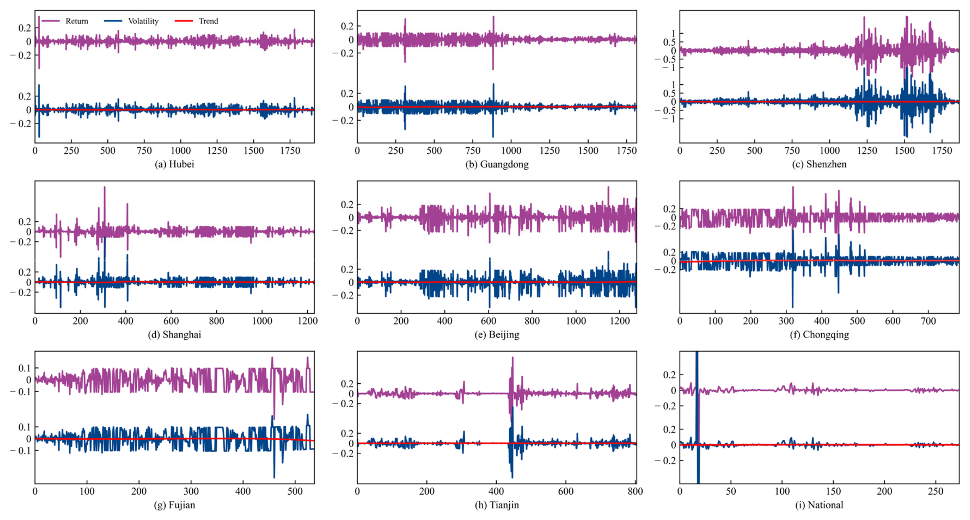
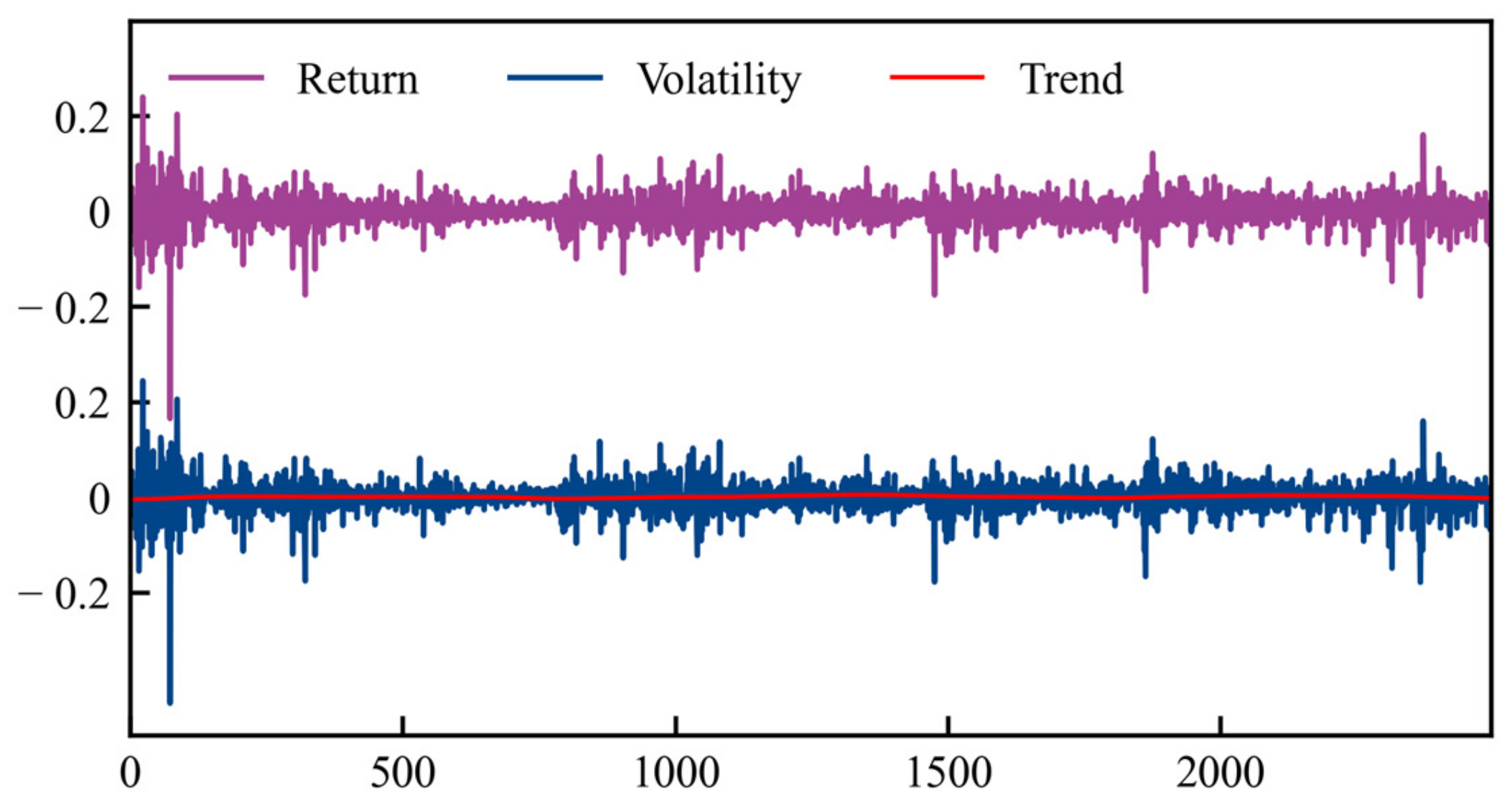
This study employs the HP filter to decompose carbon price returns into trend and volatility components, with the volatility component being closely associated with the market risk. Analysis of the volatility component of carbon price returns without the trend component enhances the understanding of the changes and trends in carbon market risks, thus facilitating an accurate risk quantification. The HP filter effectively accomplishes filtering without data loss, mitigates interference from trend components, and enhances the precision of empirical results.

(2)

This study utilizes the EGARCH model, which overcomes the shortcomings of the GARCH model in capturing asymmetry in asset returns. Additionally, EVT is incorporated to effectively address the limitation of the EGARCH model in measuring extreme tail risks. EVT provides a comprehensive consideration of extreme situations, resulting in a precise risk measurement for the Chinese carbon market.

(3)

A comprehensive assessment and comparison of volatility and risks in eight carbon pilot markets in China and in the national carbon market are conducted. Furthermore, comparisons with a mature carbon market, namely EU-ETS, are performed. This research provides policy recommendations for the future healthy development of China’s carbon market.

The remaining sections of this paper are structured as follows. Section 2 provides a detailed description of the methods employed in this study. Section 3 describes the data and data preprocessing. Section 4 presents the empirical analysis of the Chinese carbon market and EU-ETS. Section 5 provides the conclusions and policy recommendations.

2. Methodology

The logical framework of this study is shown in Figure 1. First, data are collected from eight carbon pilot markets in China, China’s national carbon market, and EU-ETS. Second, the collected carbon price time series data are transformed into a logarithmic return series and statistically tested. Then, the individual return data are de-trended using the HP filter and analyzed for volatility using EGARCH. Finally, the static and dynamic VaR of the carbon price are evaluated using EGARCH-EVT-VAR and the results are compared.

2.1. HP Filtering Method

The HP filtering method is a time series decomposition model that is generally used for the analysis of macroeconomic trends. This method was first introduced in the paper by Hodrick and Prescott (1980) [36], who studied the post-World War II U.S. economic cycle. The following is a brief description of the principle of the HP filtering method.

Let {$Y_t$} be a financial time series containing trend and volatility components, where {$Q_t$} is the trend component of the series and {$B_t$} is the volatility component of the series. Then,

$$Y_t=Q_t+B_t\hspace{1em}\mathrm{t}=1,2, \dots ,\mathrm{n}.$$

(1)

The HP filtering is used to decompose {$Q_t$} and {$B_t$} from {$Y_t$}. Generally, trend component {$Q_t$} is defined as the solution to the following minimization problem:

$$min\left\{{{\displaystyle \sum }}_{t=1}^n{\left(Y_t-Q_t\right)}^2+\lambda {{\displaystyle \sum }}_{t=1}^n{\left[c\left(L\right)Q_t\right]}^2\right\},$$

(2)

where $c\left(L\right)$ is the delay operator polynomial.

$$c\left(L\right)=\left(L^{-1}-1\right)-\left(1-L\right)$$

(3)

When Equation (3) is substituted into Equation (2), the problem of HP filtering is to minimize the following loss function:

$$min\left\{{{\displaystyle \sum }}_{t=1}^n{\left(Y_t-Q_t\right)}^2+\lambda {{\displaystyle \sum }}_{t=2}^{n-1}{\left[\left(Q_{t+1}-Q_t\right)-\left(Q_t-Q_{t-1}\right)\right]}^2\right\}.$$

(4)

The HP filtering method treats the trend component as a slowly changing element, and the allocation of data between the trend and volatility components can be adjusted using parameter λ. Commonly used λ values include 100, 1600, 14,400, and 6,812,100. As λ increases, the trend component becomes smooth, leading to high volatility. In this study, the choice of λ values is based on the characteristics of the time series data. After fine tuning the model with daily data from various carbon markets in China, the selected λ value is ultimately determined to be 6,812,100.

2.2. EGARCH

In the study of price volatility, the information that can affect the rising carbon price is called positive information, and the information that can affect the falling carbon price is called negative information. The EGARCH model [36] introduces asymmetric terms into the GARCH model and effectively overcomes the shortcomings of the GARCH model, namely the inability to describe the asymmetry of asset returns. EGARCH (1, 1) is the most commonly used among EGARCH models, and its conditional variance equation is shown as

$$ln\left({\sigma }_t^2\right)=\omega +\alpha \left|\frac{{\mu }_{t-1}}{{\sigma }_{t-1}}-\sqrt{\frac{2}{\pi }}\right|+\gamma \frac{{\mu }_{t-1}}{{\sigma }_{t-1}}+\beta ln\left({\sigma }_{t-1}^2\right),$$

(5)

where $ln\left({\sigma }_t^2\right)$ is the logarithm of the conditional variance representing the fact that the effect of leverage is exponential rather than quadratic, so the predicted value of conditional variance must be non-negative. When $\gamma \ne 0$, the effect of external shocks shows asymmetry. When $\gamma >0$, positive shocks greatly influence price volatility, and when $\gamma <0$, negative shocks greatly affect price volatility.

2.3. EVT-VaR

(1)

EVT

In the risk management of carbon markets, a common oversight occurs when the primary focus is on analyzing the overall risk while neglecting the effects of extreme risks. Extreme risks have the potential to induce sharp market price fluctuations, which can lead to substantial losses for market participants.

The tail characteristics of financial market return sequences typically differ from those of the central distribution. Therefore, a specialized method tailored for quantitatively analyzing risks in carbon markets, with a particular focus on extreme risks, needs to be established. EVT is a research methodology that specializes in quantifying losses associated with extreme risks. EVT can be classified into two categories: the block maxima method and the peak-over-threshold (POT) model. The POT model is commonly employed to measure tail-end extreme risks in financial markets. This model does not necessitate assumptions about the overall distribution of sample data and is minimally influenced by data characteristics. Thus, it has theoretical advantages over traditional models in characterizing the Chinese carbon market. This study adopts the POT model.

(2)

POT model

The POT model [37] is one of the most commonly used extreme value models and known for its ability to maximize the use of extreme value data. It can be mathematically presented as

$$\begin{gathered} G_{\xi , \beta }\left(x\right)=\left\{\begin{array}{c}1-{\left(1+\xi \frac{x}{\beta }\right)}^{-1/\xi } , \xi \ne 0;\\ 1-e^{-\raisebox{1ex}{$x$}\!\left/ \!\raisebox{-1ex}{$\beta $}\right. } , \xi =0.\end{array}\right. \\ \mathrm{when} \left\{\begin{array}{c}x\ge 0 , \xi \ge 0;\\ 0\le x\le -\beta /\xi , \xi <0.\end{array}\right. \end{gathered}$$

(6)

In Equation (6), ξ represents the shape parameter of the carbon price return distribution. Generally, when ξ > 0, $G_{\xi ,\beta }\left(x\right)$ is suitable for describing the fat-tail characteristics exhibited by the distribution of financial asset sequences. The larger the value of ξ is, the fatter the tail of the return rate is. B represents the scale parameter of the carbon price return distribution, and $\beta >0$.

(3)

Static VaR Model

VaR [38] refers to the maximum loss that a portfolio or asset composition may suffer at a given confidence level (q) in a future specific moment under the assumption of normal market fluctuations. The estimated value of static VaR_q is given as

$$Va{R}_q=\left\{\begin{array}{c}u+\frac{\beta }{\xi }\left[{\left[\frac{n}{N_u}\left(1-q\right)\right]}^{-\xi }-1\right],\xi \ne 0;\\ u-\beta ln\left(\frac{n}{N_u}\left(1-q\right)\right),\xi =0;\end{array}\right.$$

(7)

where u is the threshold, n is the sample size, $N_u$ is the number of residuals in the sequence that exceed threshold u, and q represents the confidence level. In this study, a confidence level of 95% is selected.

(4)

Dynamic VaR (EGARCH-EVT-VaR)

Dynamic VaR (EGARCH-EVT-VaR) is derived by combining the POT model from EVT with the static VaR model, resulting in a static VaR value. It also corresponds to the left quantile in Equations (8) and (9) for the carbon market. In accordance with the definition of dynamic VaR, we can calculate dynamic VaR values for upward and downward movements in carbon prices. The formulas for calculating upward and downward dynamic VaR are as follows:

$$Va{R}_t^{up}={\mu }_t-Z_q{\sigma }_t$$

(8)

$$Va{R}_t^{down}={\mu }_t-Z_q{\sigma }_t,$$

(9)

where ${\mu }_t$ represents the conditional expectation of the carbon market and Z_q is the static VaR value obtained through Equation (7). On the basis of Equations (8) and (9), we can calculate the upward and downward risks for various carbon markets in China.

The dynamic VaR model effectively captures the heteroscedasticity and asymmetry in carbon price return sequences and provides intuitive insights into the risk in the Chinese carbon market. It allows for the analysis of risk trends across different carbon markets.

2.4. Kupiec Failure Frequency Test

After the VaR estimates are calculated using the EGARCH-EVT-VaR model, an effectiveness test needs to be conducted on the VaR estimates. In this study, the chosen test method is the Kupiec failure frequency test [39], which has been widely applied in the field of financial risk management. Let D represent the number of observed sample days, and let q denote the chosen confidence level. A VaR breach occurs when the actual losses exceed the VaR estimates. Let L represent the total number of VaR breaches observed. The failure frequency, P, is defined as the ratio of the sample days to the number of VaR breaches, i.e., P = D/L.

If the VaR model is reliable, the number of breaches, N, follows a binomial distribution, where the occurrence probability of a breach is equal to failure frequency P. The probability mass function of the binomial distribution is given by

$$f\left(L\right)=\left(\begin{array}{c}D\\ L\end{array}\right)P^D{\left(1-P\right)}^{D-L}.$$

(10)

The expected failure frequency is denoted as E(P) = 1 − P. When the actual VaR failure frequency is greater than the expected failure frequency, the market risk is underestimated by the VaR model; the opposite suggests an overestimation of the market risk. The closer the actual VaR failure frequency is to the expected failure frequency, the higher the effectiveness of the VaR model is. Kupiec constructed a test statistic, LR, to evaluate

$$LR=-2ln\left[{\left(1-P\right)}^{D-L}{P}^L\right]+2ln\left[{\left(1-\frac{D}{L}\right)}^{D-L}{\left(\frac{D}{L}\right)}^L\right].$$

(11)

Under the null hypothesis, the LR statistic follows a chi-squared distribution with one degree of freedom. Given a confidence level of q, we compare the LR value with the critical value to determine whether to reject the null hypothesis. When the LR value is greater than the critical value, we reject the null hypothesis and do not accept the VaR estimate, indicating that the model used to measure the carbon market risk is unreliable. Conversely, when the LR value is less than the critical value, we accept the VaR estimate, signifying that the model used to assess the carbon market risk is reliable.

3. Data Preprocessing

3.1. Data Source

This study used data on eight carbon trading pilot markets in China as research objects; the eight markets were Hubei, Guangdong, Shenzhen, Shanghai, Beijing, Chongqing, Fujian, and Tianjin. The eight pilot carbon markets cover the main carbon-emitting sectors and are mainly based on free allocation. Additionally, China’s national carbon market, which officially launches on 16 July 2021, covers mainly the power sector, with free and ex-post allocations, resulting in a relatively low carbon price in China, and there is greater fluctuation in the Chinese carbon market, especially short-term shocks [40]. The daily closing prices of each carbon market were selected, and dates with zero trading volume were excluded. The time frame ranged from the establishment of each carbon market to 31 August 2022, and the data source was the China Emissions Exchange (www.tanpaifang.com, 15 September 2022). Natural logarithm returns were used as the daily returns for carbon prices. The daily return curves for each carbon market are shown in Figure 2. Hubei’s carbon price return sequence exhibited dense fluctuations. It presented a considerable change in the early period but showed a certain regularity overall. Guangdong’s carbon price return had two nodes with large fluctuations in the volatility component; it presented considerable initial volatility, followed by a gradual reduction and convergence. By contrast, Shenzhen’s carbon price return showed initial stability, with the latter periods experiencing increasing volatility, before returning to a stable state. Shanghai’s carbon price return had a series of sharp fluctuations in the early period, followed by a gradually stabilizing trend in volatility. Beijing’s carbon price return exhibited long-term substantial fluctuations, indicating high sensitivity to carbon price changes. In the case of Chongqing and Fujian, the two markets experienced multiple abrupt changes due to low trading volumes, discontinuous trading, and overall low activity, leading to jumps in their return volatility components. Tianjin’s carbon price return volatility component was relatively stable in the early period but exhibited considerable changes in the mid-term, followed by gradual stabilization. The national carbon market, being relatively new, initially had one highly volatile node, followed by a period of relative stability.

The overall changes in the yield sequences of carbon markets in China showed that a decrease in market activity leads to an increase in the overall volatility of the carbon market. As the trading volume in the carbon market continues to rise and as market development becomes increasingly robust, the market’s ability to withstand risks improves. By contrast, when affected by external shocks, carbon markets with low activity and risk resilience struggle to absorb the sharp fluctuations in carbon prices, resulting in an increased market risk and a vicious cycle. This observation is particularly evident in the case of the Chongqing and Fujian carbon markets. As shown in Figure 2, the volatility components of carbon price returns in Chongqing and Fujian exhibit excessive and erratic changes and even experience cliff-like drops without clear volatility patterns that surpass the normal range of market fluctuations. Rapid changes in carbon price returns inevitably increase the market risk and reduce the carbon market trading volume, making the market susceptible to a vicious cycle.

3.2. HP Filter Rejection Trend Processing

Carbon price yield variations can be viewed as a combination of trend and volatility components, with the yield volatility component being related to the market risk. Studying the volatility component increases the understanding of the changes and trends in carbon market risk, thereby improving market risk measurement. The trend component must be extracted from the carbon price yield sequence and removed, focusing solely on the analyzed yield volatility component. The HP filtering method can perform filtering without data loss and effectively mitigate the effect of the trend component on the analysis results. To accurately measure the risk situation in the Chinese carbon market and avoid the influence of the trend component on the subsequent calculation of VaR values, this study used HP filtering to decompose yield data, remove the trend component, and retain the volatility component of the carbon price yield. Given that the data were daily, a λ value of 6,812,100 was selected. The decomposition results of HP filtering are shown in Figure 2. Figure 2 indicates that a trend component still exists in the original yield series and needs to be removed. The descriptive statistics of the yield volatility component data for each carbon market after the trend component is removed are shown in

Table 1. Descriptive Statistics of Return Volatility Components in Chinese Carbon Trading Markets.

Carbon Trading Market	Sample Size	Mean	Standard Deviation	Skewness	Kurtosis	J-B Test
Hubei	1917	0.0000	0.0336	−0.1544	23.0059	31,976.54 (0.0000)
Guangdong	1816	0.0000	0.0456	−0.5078	12.9327	7543.151 (0.0000)
Shenzhen	1865	0.0000	0.2777	−0.0435	19.1561	20,284.05 (0.0000)
Shanghai	1230	0.0000	0.0683	1.5487	37.6493	62,021.13 (0.0000)
Beijing	1278	0.0000	0.0870	−0.3684	5.8054	448.0050 (0.0000)
Chongqing	787	0.0000	0.1398	−0.6181	8.8495	1172.118 (0.0000)
Fujian	537	0.0000	0.0717	−0.2503	2.7632	6.8604 (0.0000)
Tianjin	804	0.0003	0.0698	−0.1752	42.0751	51,153.90 (0.0000)
China	276	0.0000	0.1995	−0.2399	133.6022	194,025.3 (0.0000)

. According to Table 1, the mean of the yield volatility component for all carbon markets is 0. The large standard deviation indicates high yield volatility. Skewness is nonzero for all markets, except for the Shanghai carbon market, suggesting left-skewed characteristics for all markets except Shanghai. The kurtosis values for all carbon trading markets, except for the Fujian carbon market, exceed 3. The J-B values for all carbon markets in China are greater than the critical value. These results indicate that the yield volatility component in the Chinese carbon markets exhibits notable peak-heavy-tail characteristics. Therefore, the distribution of carbon price yields differs considerably from the normal distribution and exhibits substantial risk characteristics.

3.3. Stationarity and ARCH Effect Test

Before an empirical analysis, a stationary test must be performed on the yield volatility components of carbon prices in the various Chinese carbon markets. This study used the augmented Dickey–Fuller (ADF) test to examine the stationarity of the yield return series of carbon prices, and the test results are presented in

Table 2. ADF Test Results.

Carbon Markets	Test Statistic	1%	5%	10%	Probability	Conclusion
Hubei	−51.8254	−3.9628	−3.4122	−3.1280	0.0000	stable
Guangdong	−44.6094	−3.9631	−3.4123	−3.1281	0.0000	stable
Shenzhen	−28.9288	−3.9629	−3.4122	−3.1280	0.0000	stable
Shanghai	−20.7942	−3.9656	−3.4125	−3.1288	0.0000	stable
Beijing	−29.1092	−3.9652	−3.4133	−3.1287	0.0000	stable
Chongqing	−13.1804	−3.9698	−3.4156	−3.1300	0.0000	stable
Fujian	−17.4629	−3.9753	−3.4182	−3.1316	0.0000	stable
Tianjin	−37.7743	−3.4383	−2.8649	−2.5686	0.0000	stable
China	−12.3683	−3.9927	−3.4267	−3.13659	0.0000	stable

.

Table 2 shows that the ADF values of the yield volatility components in the various carbon markets are significantly lower than the critical values at the 1%, 5%, and 10% significance levels. This finding indicates a strong statistical significance and rejection of the null hypothesis, suggesting the absence of a unit root and the presence of stationarity characteristics in these yield volatility components. Therefore, models can be established for the yield volatility components of the nine regional carbon trading markets in China.

An ARCH effect test needs to be conducted on the yield volatility components of the various carbon markets in China before using the EGARCH model because of the presence of significant volatility clustering characteristics in the capital market time series data. The ARCH effects are tested using the fitted residual sequences, and the results are presented in

Table 3. ARCH Effect Test Results.

Carbon Markets	F-Statistic	Prob. F	Obs∗R-Squared	Prob. Chi-Square
Hubei	531.0208	0.0000	416.1256	0.0000
Guangdong	103.5125	0.0000	98.0297	0.0000
Shenzhen	438.5068	0.0000	355.3029	0.0000
Shanghai	95.5243	0.0000	88.7691	0.0000
Beijing	375.3255	0.0000	290.5247	0.0000
Chongqing	115.7247	0.0000	101.0971	0.0000
Fujian	39.9024	0.0000	37.2671	0.0000
Tianjin	155.8933	0.0000	434.3331	0.0000
China	282.3283	0.0000	67.0057	0.0000

.

As shown in Table 3, the p-values for the F-test statistic and the chi-square test statistic for the yield volatility components of each carbon market are 0. This finding indicates that at the 5% significance level, the null hypothesis is rejected for all carbon markets, implying that the yield volatility components of each carbon market exhibit significant ARCH effects.

4. Empirical Analysis

4.1. Empirical Results on the Carbon Market in China

4.1.1. Parameter Estimation of the EGARCH Model

The yield volatility components of all the carbon markets in China are stationary time series and exhibit ARCH effects, which are in line with the modeling conditions of the EGARCH model. This study selected the order of the EGARCH model on the basis of the principle of minimizing the Akaike information criterion and the Bayes information criterion. The EGARCH (1, 1) model under the assumption of normal distribution was chosen to estimate the yield series of the nine carbon markets in China. The parameter estimation results of the EGARCH (1, 1) model for each carbon market are shown in

Table 4. Parameter Estimation Results of the EGARCH (1, 1) Model for China’s Carbon Markets.

Parameters	Hubei	Guangdong	Shenzhen	Shanghai	Beijing	Chongqing	Fujian	Tianjin	China
$\mu$	0.0000	0.0000	0.0000	0.0000	0.0000	0.0000	0.0000	0.0000	0.0000
	(1.0000)	(1.0000)	(1.0000)	(1.0000)	(1.0000)	(1.0000)	(1.0000)	(1.0000)	(1.0000)
$\omega$	−0.6540	−0.6356	−0.2676	−0.4851	−0.4515	−0.3778	−0.5570	−0.5915	−0.8010
	(0.0000)	(0.0000)	(0.0000)	(0.0000)	(0.0000)	(0.0317)	(0.0276)	(0.0000)	(0.0000)
$\alpha$	0.0401	0.0575	−0.0053	0.0400	−0.0018	0.0081	0.0298	−0.0679	−0.2988
	(0.0273)	(0.0256)	(0.8792)	(0.1258)	(0.9500)	(0.7920)	(0.4136)	(0.0900)	(0.0000)
$\beta$	0.8993	0.9010	0.9078	0.9000	0.9001	0.9116	0.8996	0.9000	0.9002
	(0.0000)	(0.0000)	(0.0000)	(0.0000)	(0.0000)	(0.0000)	(0.0000)	(0.0000)	(0.0000)
$\gamma$	0.3557	0.6467	0.6826	0.4729	0.4781	0.4734	0.3633	0.6589	0.4055
	(0.0000)	(0.0000)	(0.0000)	(0.0000)	(0.0000)	(0.0000)	(0.0000)	(0.0000)	(0.0000)
AIC	−4.2426	−4.0468	−0.8570	−3.0355	−2.5120	−1.3515	−2.5970	−4.0620	−5.1516
BIC	−4.2281	−4.0316	−0.85702	−3.0147	−2.4919	−1.3219	−2.5571	−4.0329	−5.0861
L-K	4077.89	3683.52	804.17	1876.37	1614.00	537.50	702.30	1637.94	715.93

Note: $\alpha$ is the coefficient of the ARCH term, $\beta$ is the coefficient of the GARCH term, $\gamma$ is the coefficient of the leverage term, and the test p-values are in parentheses, AIC is the Akaike information criterion, BIC is the bayesian information criterion, L-K is the likelihood estimate.

.

Table 4 shows that at the 95% confidence level, the ARCH coefficients of Hubei, Guangdong, Shanghai, Chongqing, and Fujian carbon markets are all greater than zero, indicating that past volatile disturbances in the five markets have a positive effect on future market volatility. Additionally, these markets exhibit characteristics of volatility clustering, meaning that significant fluctuations tend to follow one another closely and provide speculative incentives for investment groups in the carbon market. The parameters and their sums for all carbon markets in China are close to 1, suggesting that price volatility across these markets displays persistence, conditional heteroscedasticity, and aggregation. This observation implies that price volatility is persistent and that the markets exhibit a long memory. The parameters are all negative and statistically significant, indicating that Chinese carbon markets have relatively high risk levels. The leverage coefficient is greater than zero and statistically significant, implying the presence of significant leverage effects in Chinese carbon markets that are positive in nature. When external shocks affect Chinese carbon markets, the rate of price reversion to the mean tends to be relatively low, indicating a weak self-regulating capacity in the current carbon markets. They exhibit some degree of lag and long-term memory in price volatility. For instance, changes in market mechanisms, adjustments to quota allocation policies, and climate variations can all affect carbon prices, leading to fluctuations. Furthermore, when external shocks dissipate, the considerable price fluctuations do not immediately disappear due to their prolonged effect, indicating that volatility persists for some time. Consequently, when carbon prices exhibit high volatility, the overall market risk becomes increasingly pronounced.

4.1.2. Static VaR Estimation Results

In this study, the maximum standardized residual of 10% was selected for tail modeling and tail threshold estimation, and R software was used to estimate the shape and scale parameters of the POT model in EVT. The results of the parameter estimation are shown in

Table 5. Parameter Estimation Results of the POT Model.

Carbon Markets	$\widehat{\mathit{\beta }}$	$\widehat{\mathit{\xi }}$	$\mathit{V}\mathit{a}{\mathit{R}}_{0.95}$
Hubei	0.6322	0.2577	1.5957
Guangdong	0.6962	0.1844	1.5228
Shenzhen	0.4648	0.3752	1.3453
Shanghai	0.3607	0.4619	1.0536
Beijing	0.3760	0.2595	1.0996
Chongqing	0.2062	0.3468	1.0201
Fujian	0.2956	0.0490	0.9753
Tianjin	0.6431	−0.1889	0.8544
China	0.4567	0.6023	0.0294

.

Table 5 shows that the fitting results of the shape parameters of the carbon markets in China, except for the Tianjin carbon market, are all positive, which further confirms that the fluctuation of carbon price yield in most carbon markets in China has a thick tail. At the 95% confidence level, the static VaR value of the Hubei carbon market is the highest, with 95% assurance that the maximum loss caused by its price fluctuation will not exceed 1.5957%. The static VaR value of the national carbon market is the lowest, with 95% assurance that the maximum loss caused by its price fluctuation will not exceed 0.0294%. However, due to the large differences in carbon prices in the various markets, the static VaR estimates of the various markets cannot be directly used for a horizontal comparison, nor can they be used for a direct comparison of the risk situation. Therefore, the VaR of the carbon markets needs to be dynamically fitted to show the change in VaR in each market and judge the change in the fluctuation risk in each market.

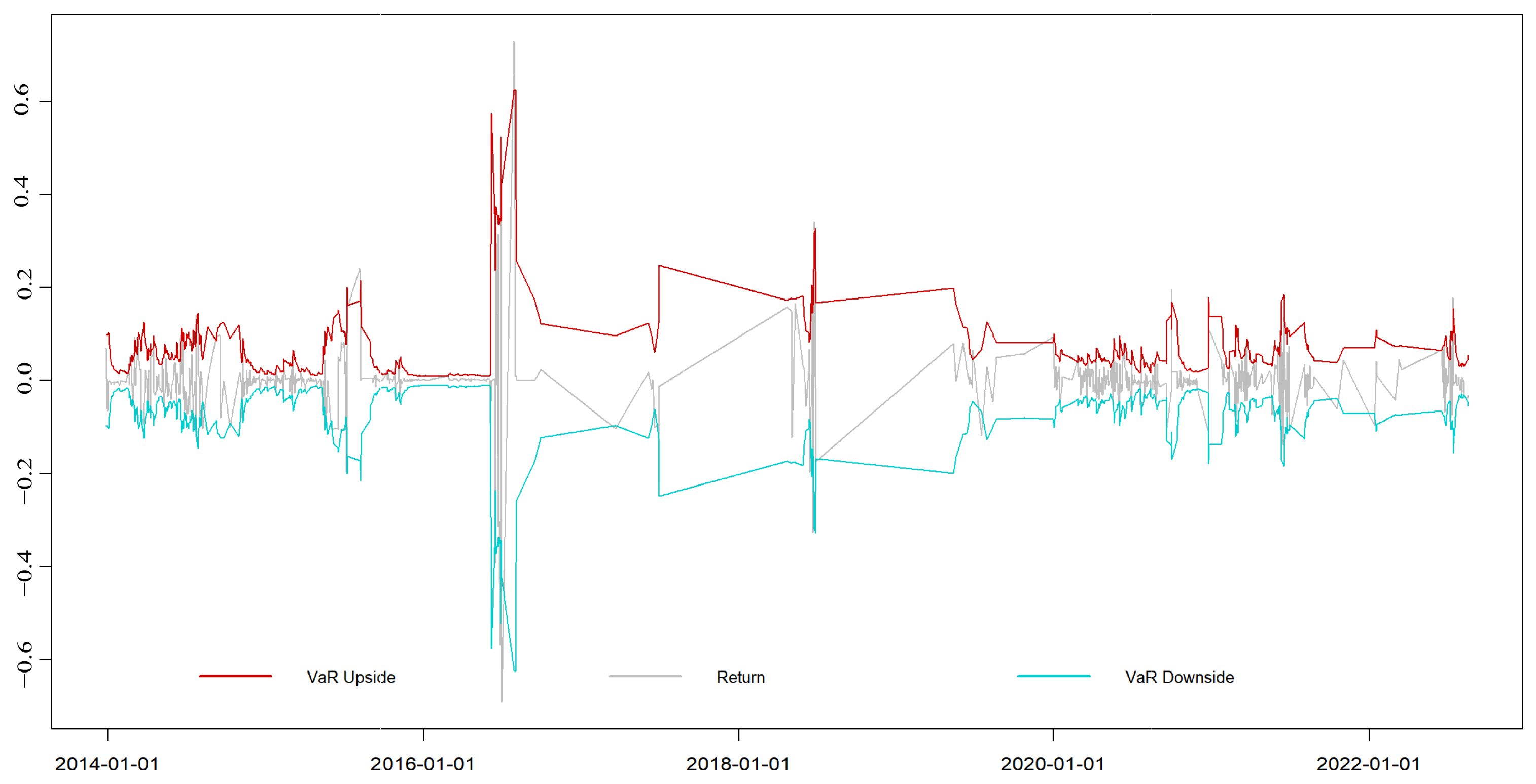
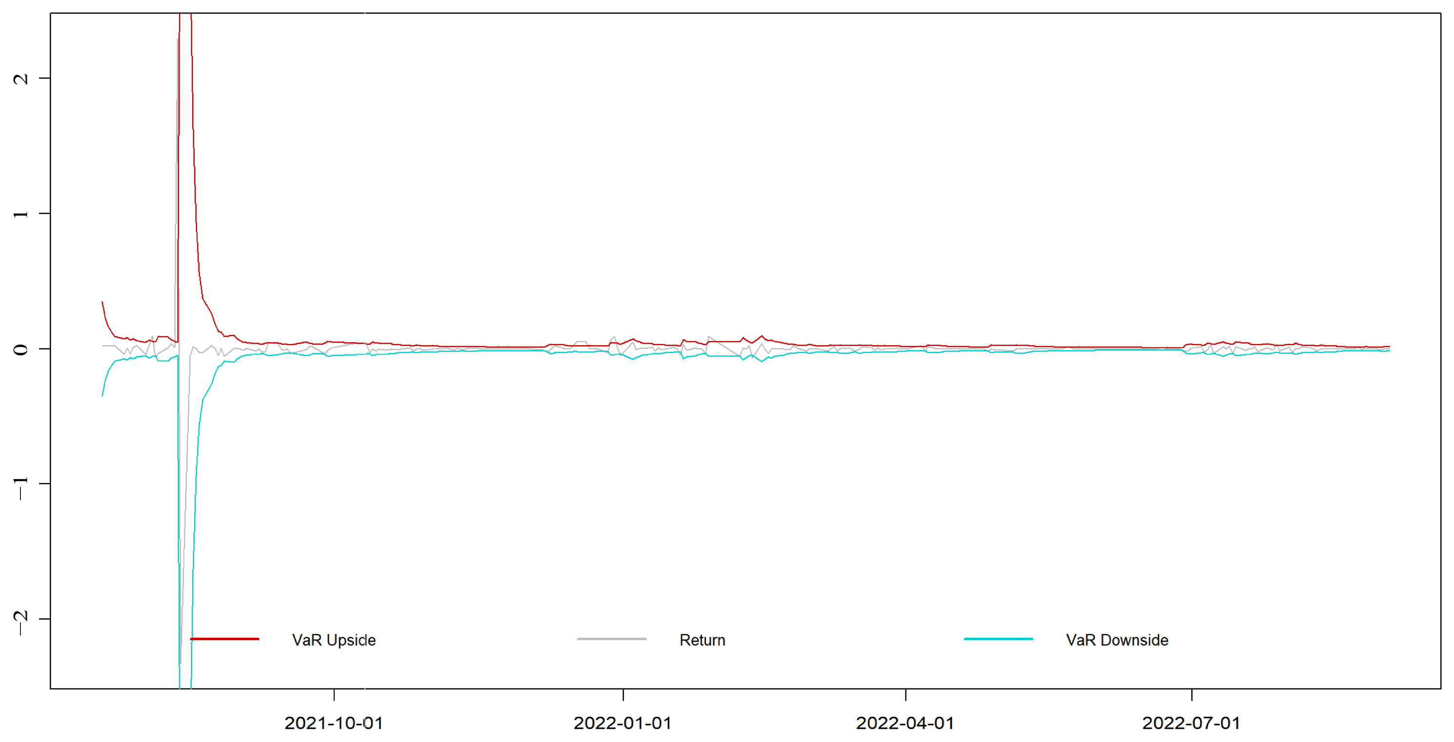
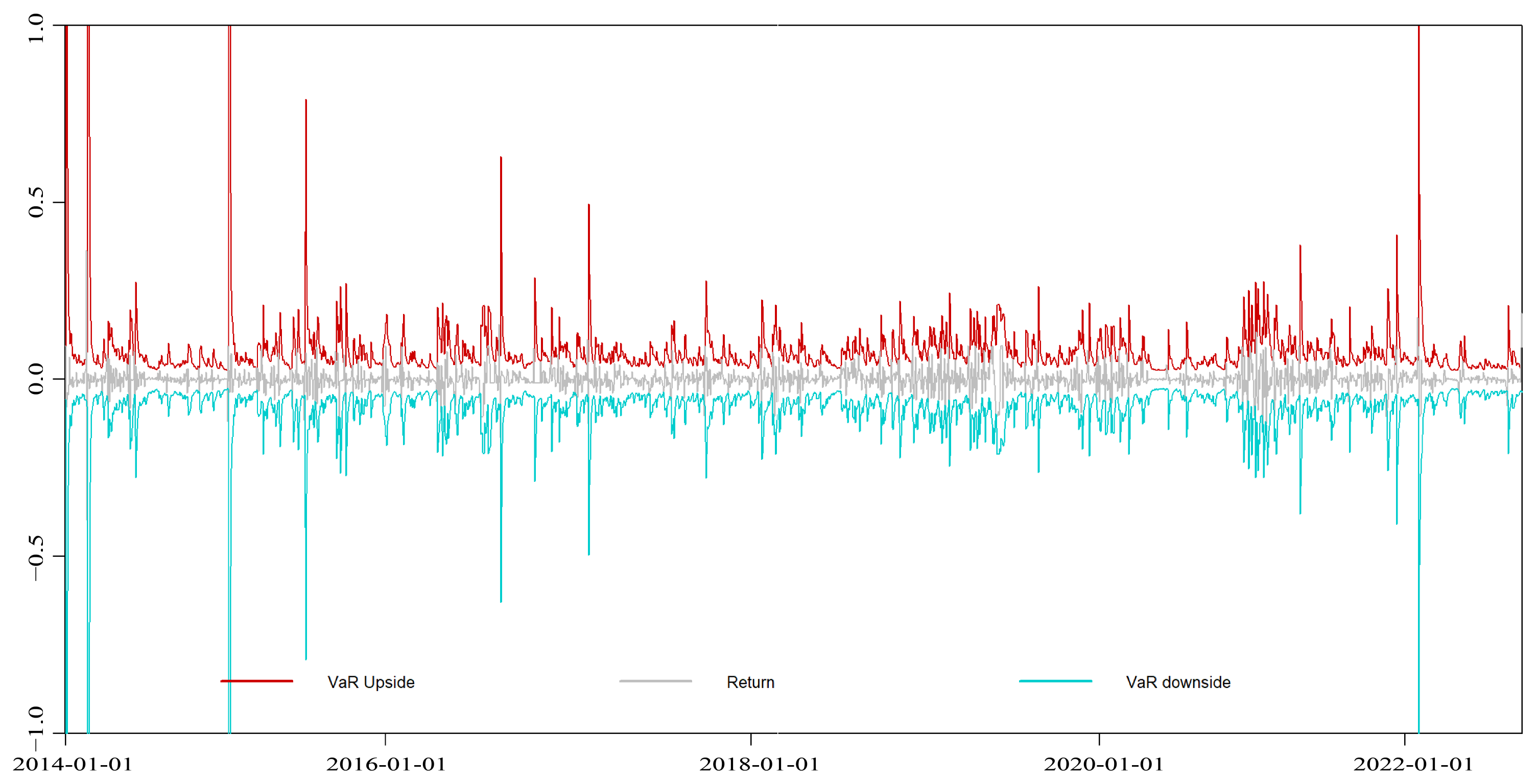
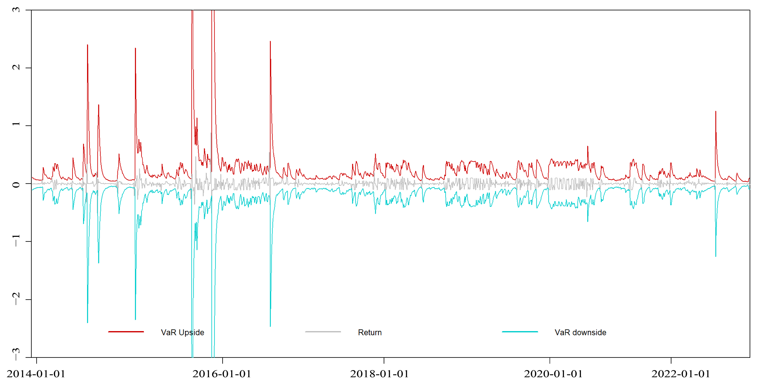
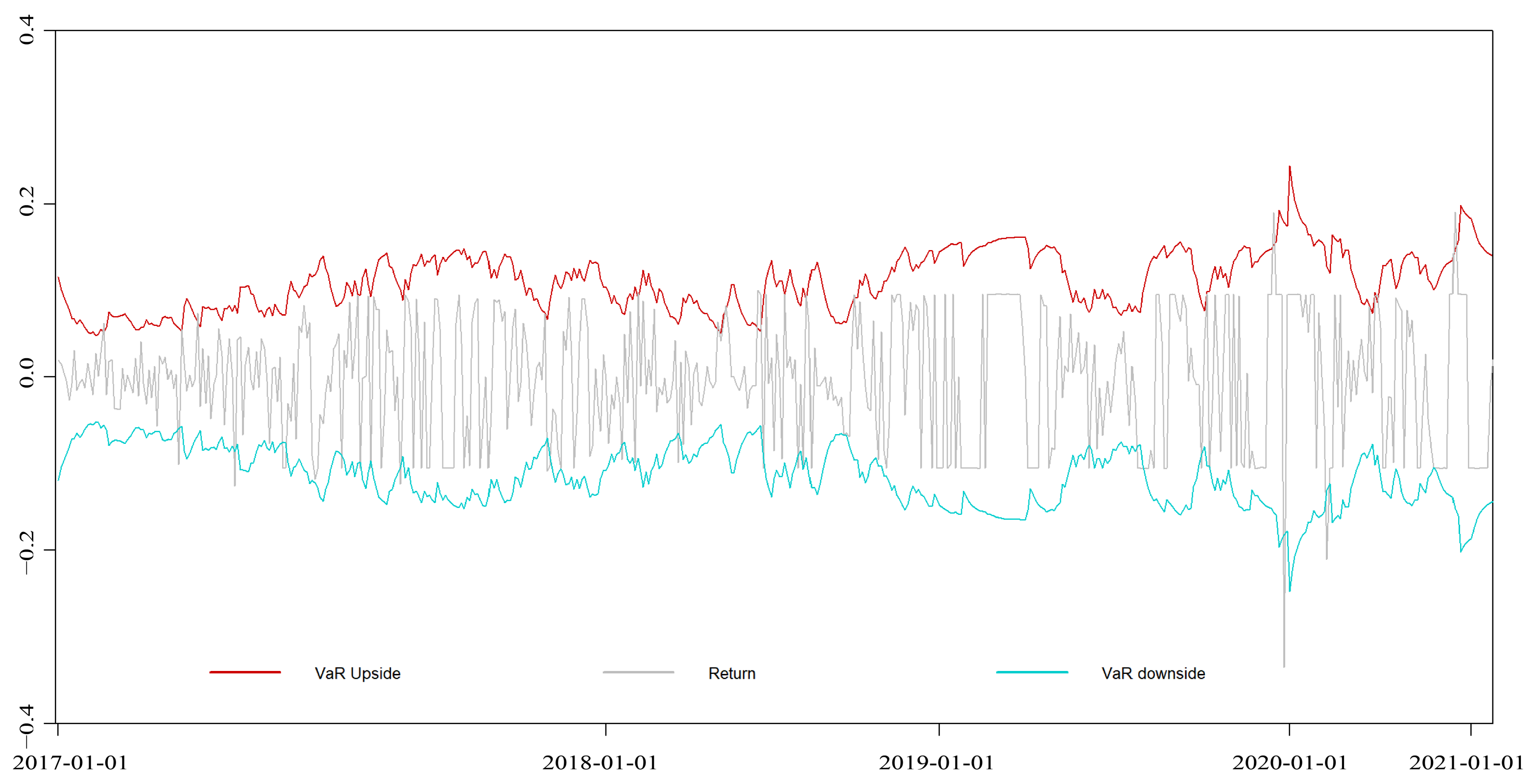
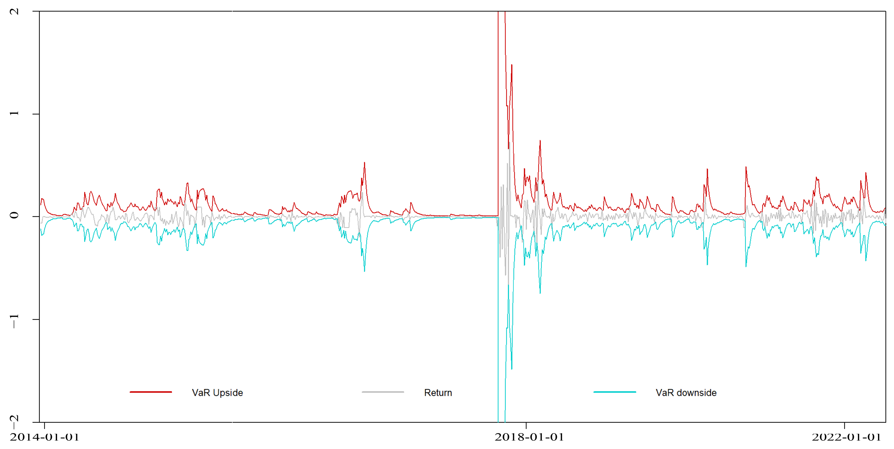
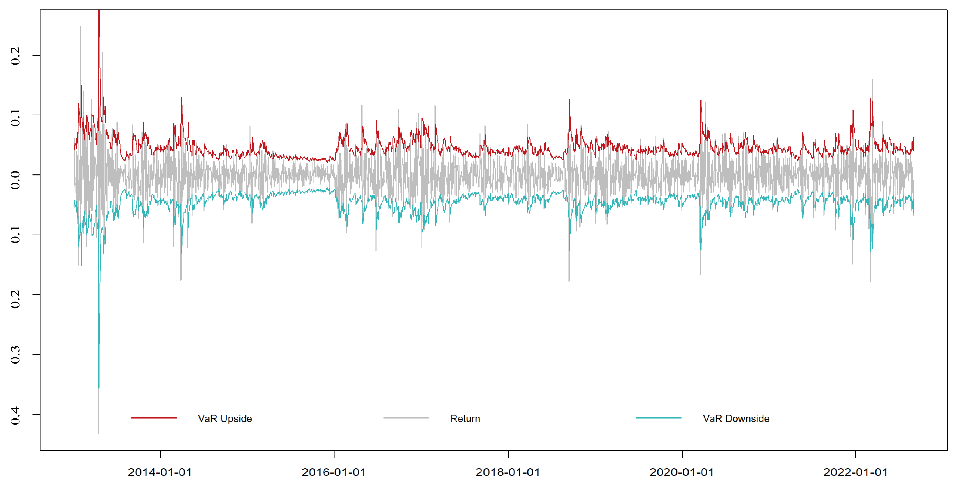
4.1.3. Dynamic VaR Estimation Results

A description and a statistical analysis of the dynamic VaR values of the various carbon markets in China at the confidence level of 95% are shown in

Table 6. Statistics of VaR Value Measurement Results of Various Carbon Markets in China.

Carbon Markets	Averages	Max.	Min.	Standard Deviation	Skewness	Kurtosis
Hubei	0.0506	0.5744	0.0198	0.0261	7.9355	129.0302
Guangdong	0.0613	0.5183	0.0118	0.0403	2.2107	13.5942
Shenzhen	0.2851	3.7000	0.0445	0.2831	4.0066	25.7141
Shanghai	0.0786	1.9655	0.0222	0.0826	13.6247	266.6291
Beijing	0.1024	0.3997	0.0285	0.0579	1.0232	1.1268
Chongqing	0.1636	0.7989	0.0617	0.0672	2.6965	18.6657
Fujian	0.0916	0.2305	0.0414	0.0273	0.5495	0.5331
Tianjin	0.0618	0.6258	0.0098	0.0653	4.1686	25.3294
China	0.0608	2.9391	0.0074	0.2479	9.5951	98.1866

.

As shown in Table 6, the risk values of the carbon markets in China differed, with the maximum value of VaR being 3.7000 and the minimum value being 0.2305. The greater the standard deviation is, the greater the level of market fluctuation. Among the carbon markets, Shenzhen has the largest standard deviation and market fluctuation, and Hubei has the smallest standard deviation and market fluctuation. The VaR estimates of the nine carbon markets in China are all right-biased, and many extreme values are on the right-hand side of the overall data. Except for the data kurtosis of Beijing and Fujian carbon markets, the data kurtosis of the other carbon markets in China is relatively large, indicating that the risk fluctuates sharply.

The rising and falling dynamic VaR values of the national carbon market and each pilot carbon market from 2013 to 2022 at the 95% confidence level were calculated by constructing an EGARCH-EVT-VaR model, and the dynamic VaR of the actual carbon price return rate of each carbon market in China was fitted. The fitting results are shown in Appendix A.

As shown in Appendix A, the EGARCH-EVT-VaR model constructed in this study fits the fluctuation of returns in the various carbon markets well. When the return series fluctuates violently, the dynamic VaR value also fluctuates violently, so dynamic VaR effectively reflects the fluctuation of returns under the given carbon price.

From a holistic perspective, the risk dynamics across different carbon markets in China presented considerable variation with low inter-market correlations. No apparent overall convergence was observed in risk dynamics. Only the nationwide carbon market experienced an abrupt upsurge followed by a rapid decline in risk during its initial phase; it subsequently transitioned to a state of stability and maintained minor fluctuations. By contrast, the other carbon markets exhibited substantial variations in volatility. To obtain deep insights into the risk dynamics of China’s carbon markets and explore their underlying causes, this study divided the research period into three distinct phases: the pilot carbon market development phase, the launch phase of the national carbon market, and the phase of nationwide carbon market development. Each of these phases was comprehensively examined and discussed.

(1)

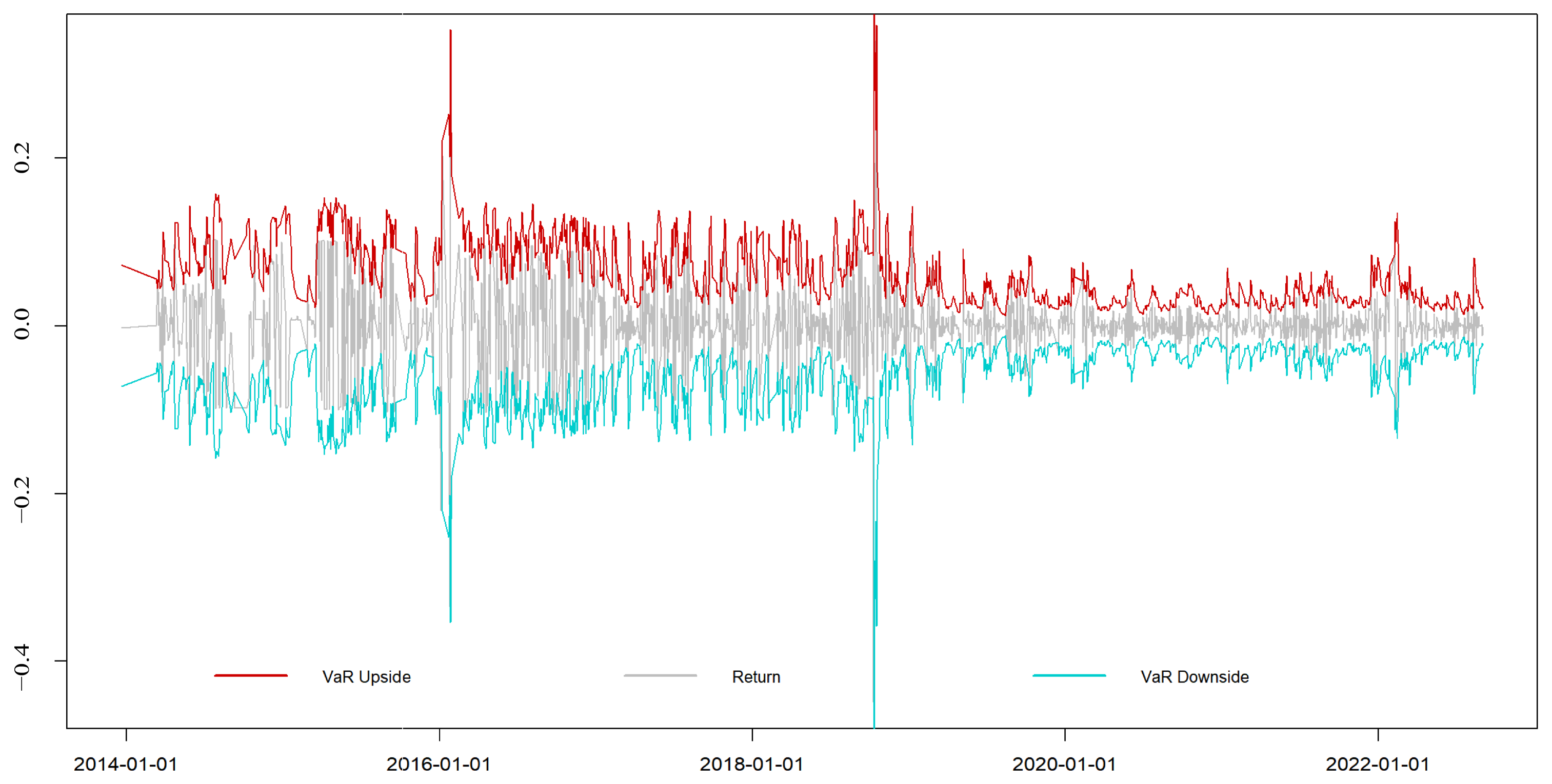
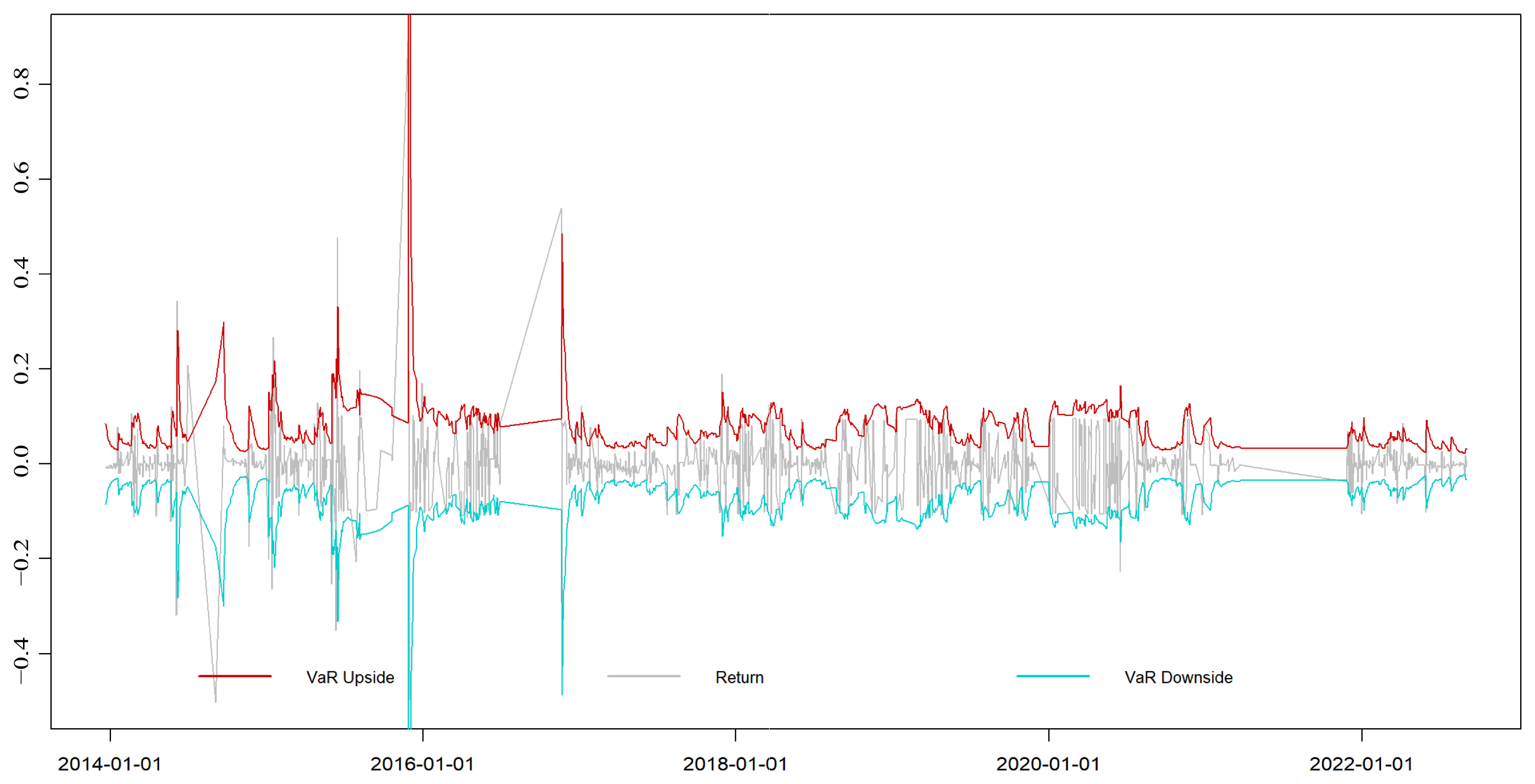
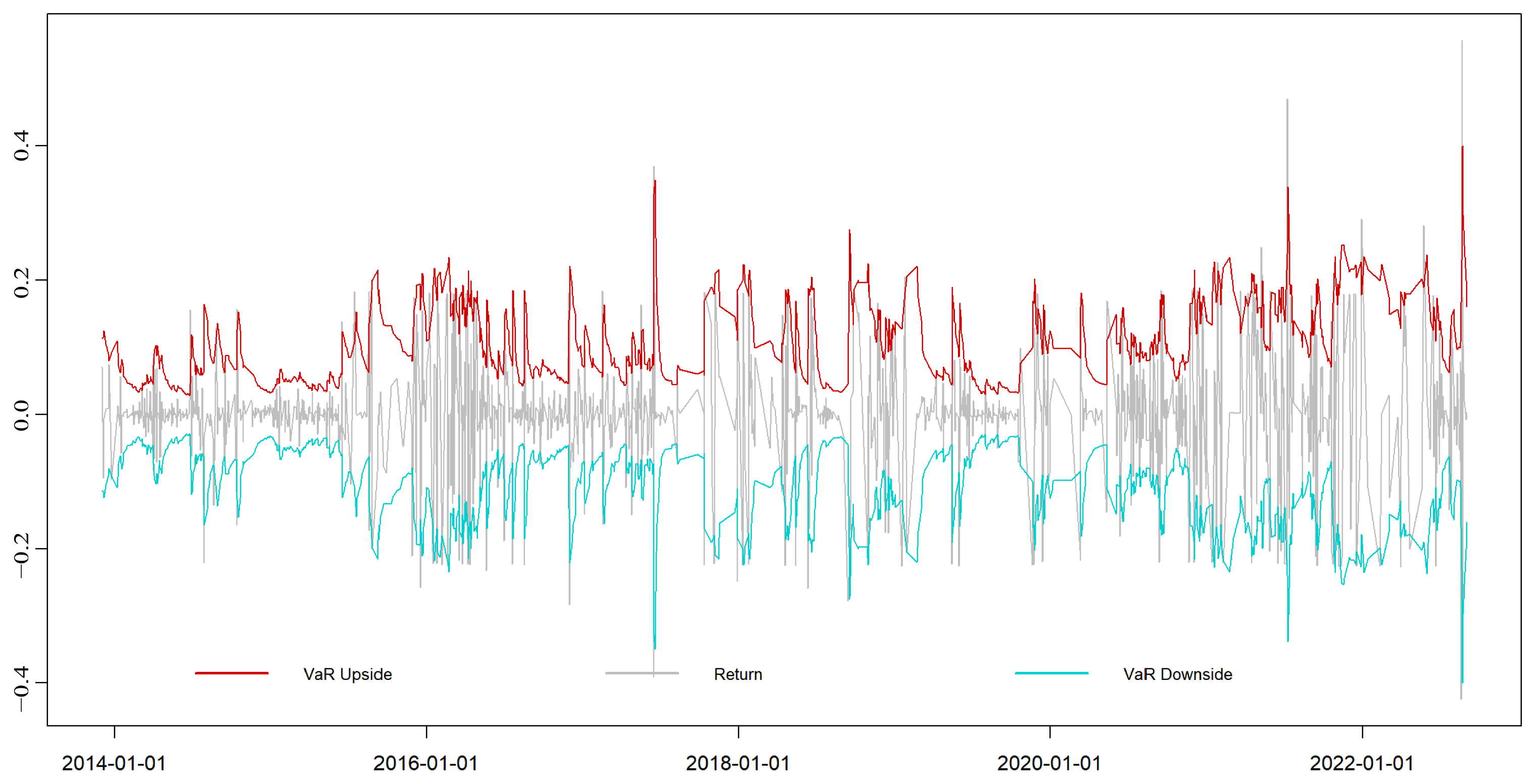
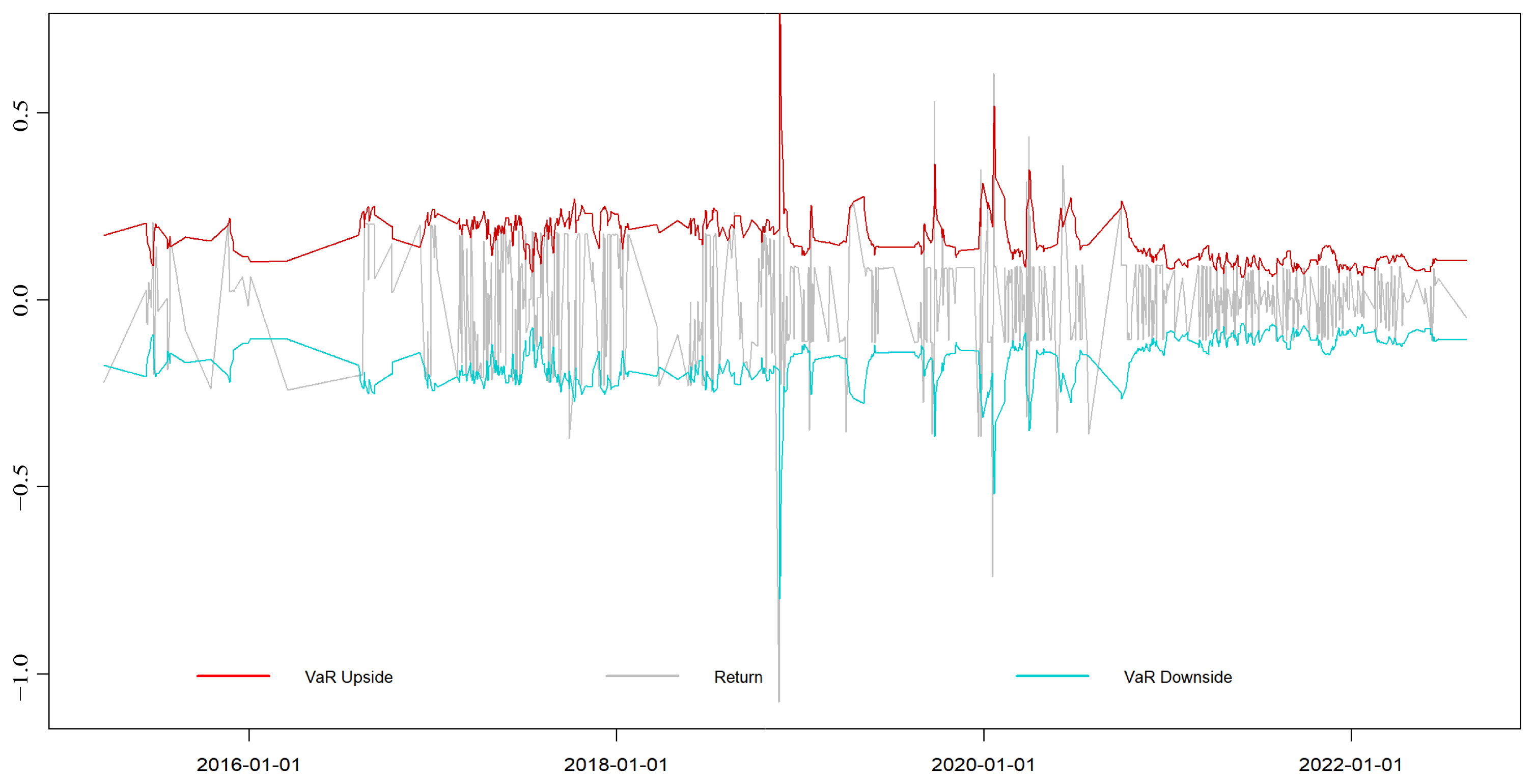
Pilot carbon market development phase (2013–2016). The period from 2013 to 2016 marked the initial development phase of carbon markets in China. During this phase, the establishment of various pilot carbon markets elicited considerable attention, and policies related to carbon trading were gradually introduced. The risk profiles of carbon markets in Hubei, Guangdong, and Shenzhen remained stable during this stage primarily because of the effective risk management measures implemented in these regions. Although the risks in the Shanghai and Beijing markets remained stable and within a manageable range throughout this period, with no notable abnormal fluctuations, they exhibited higher levels of risk volatility compared with the risks in the Hubei, Guangdong, and Shenzhen carbon markets. By contrast, the carbon markets in Chongqing, Fujian, and Tianjin experienced overall substantial fluctuations and high market risks. VaR exhibited several abrupt changes, indicating unfavorable performance overall. In the case of the Fujian carbon market, which was at its nascent stage during this period, its available carbon price data were lacking, so its risk dynamics could not be examined. In summary, during the pilot carbon market development phase, variations in the geographical conditions and resource endowments of each carbon pilot market led to distinct characteristics in risk volatility, resulting in different evolution trends.

(2)

National carbon market launch phase (2017–2020). China began the construction of a national carbon market at the end of 2017, and after nearly four years of pilot operation, it was officially launched in July 2021. During this phase, the risk profile of the Hubei carbon market continued to exhibit a stable development trend. VaR did not experience considerable fluctuations and remained stable. This stability can be attributed to Hubei’s industrial base and industrial structure, which ensure the vibrancy of carbon trading and price stability. The risk in the Guangdong carbon market, with the smallest carbon price fluctuations and the highest level of risk management, showed a gradual decline. The Shenzhen carbon market, which is currently the most remarkable carbon market in China, experienced intense volatility and abrupt changes in its dynamic VaR. The magnitude of risk variation was unprecedented, indicating the market’s sensitivity to policy changes. The establishment of the national carbon market considerably affected carbon trading in this region. The Shanghai carbon market did not exhibit substantial changes. Unlike risk volatility, dynamic VaR decreased and remained stable without considerable fluctuations. This finding suggests that the construction of the national carbon market has a positive effect on the Shanghai market. Although Beijing is not the primary carbon market in China, its unique location exposed it to the largest-ever market risk changes. The carbon markets in Chongqing, Fujian, and Tianjin, due to their limited trading volumes and low market activity, were minimally affected. From the perspective of risk changes in China’s pilot carbon markets, the establishment of the national carbon market had a direct effect on these pilot markets, and this influence is expected to persist for a long period. Therefore, facilitating the smooth transition of pilot carbon markets to the national carbon market is a challenge for China as it promotes long-term low-carbon economic development.

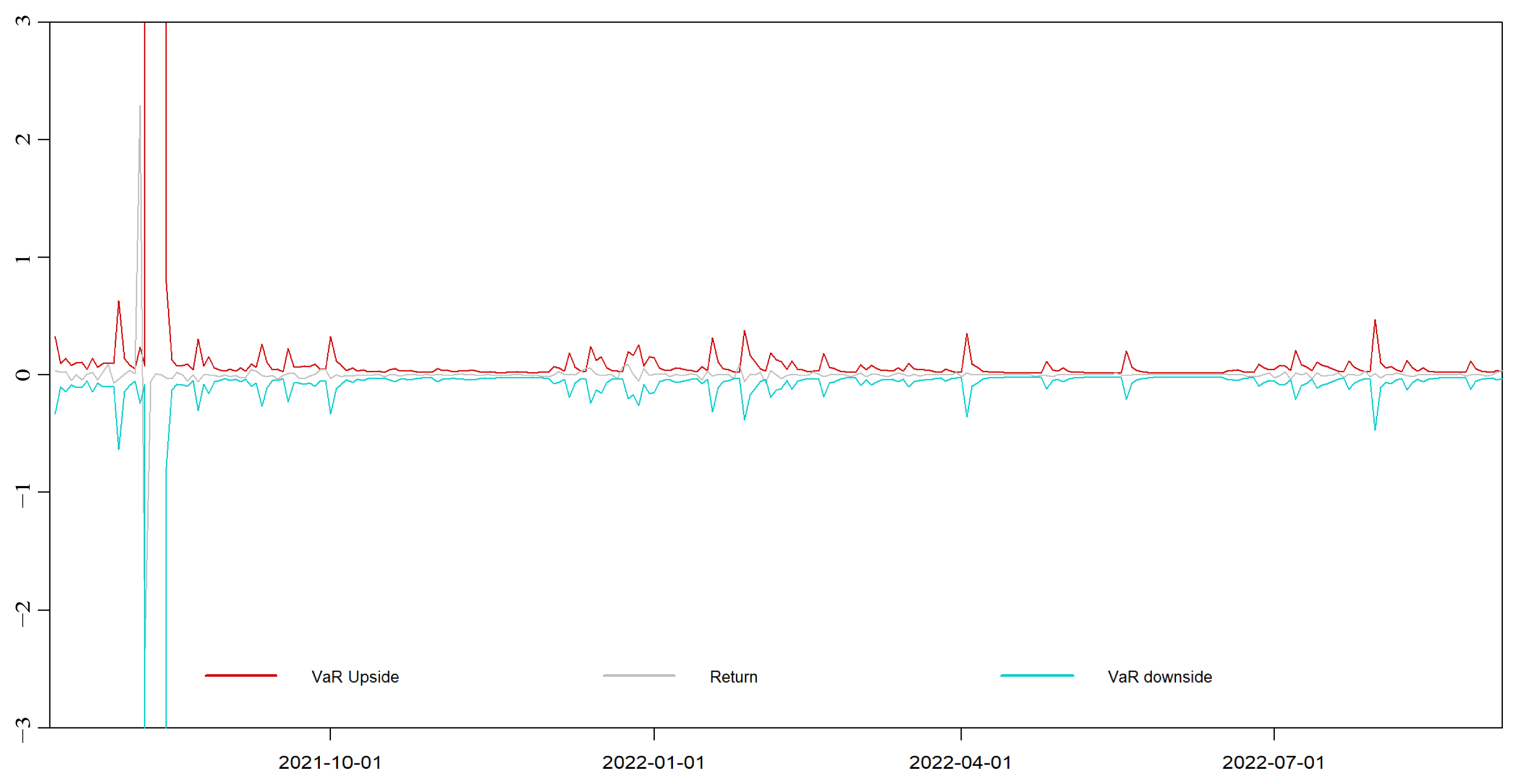
(3)

National carbon market development phase (2021–present). During this phase, the carbon markets in the pilot regions of Hubei and Guangdong generally showed stable development trends. Their risk management levels were high, and the carbon markets operated well. By contrast, the Shenzhen carbon market had the highest degree of volatility and volatility intensity among all the pilot carbon markets, resulting in an overall higher risk. The Shanghai carbon market demonstrated stability. Its dynamic VaR gradually decreased, and volatility was gradually mitigated, with the market risk remaining within manageable limits. Beijing’s carbon market, due to its unique location and sensitivity to policy changes, experienced considerable risk fluctuations. Additionally, the economic environment underwent substantial changes due to the pandemic, which further affected the market. The combination of these factors led to a substantial increase in risk in the Beijing carbon market. The risk dynamics of Tianjin and Chongqing carbon markets improved slightly during this phase compared with the risk dynamics in the two previous phases; volatility was reduced, and no abrupt changes occurred. With regard to the Fujian carbon market, its risk dynamics after 13 January 2021, could not be analyzed due to the absence of carbon price data. The national carbon market experienced one notable fluctuation event at the beginning of trading, followed by an immediate reduction in volatility. Afterward, it maintained relatively minor fluctuations, demonstrating an overall stable trend.

In summary, from 2013 to the present, the carbon markets in Hubei and Guangdong demonstrated the highest levels of risk management among all carbon markets in China. Despite remarkable early fluctuations, these markets maintained a stable development trend and presented a converging pattern over time. The performance of the Shenzhen carbon market was the opposite of the performance of the Hubei and Guangdong markets, with low volatility at its early stages and considerable increments in volatility at the latter stages. It exhibited the highest volatility among all the carbon markets and had a higher overall risk. Meanwhile, the Shanghai carbon market showed a consistent risk pattern, with volatility consistently staying within a certain range and with no notable abnormal fluctuations. The Beijing carbon market was considerably affected by policy changes, resulting in notable risk fluctuations, especially after the release of documents related to the establishment of the national carbon market, which had a particularly strong influence. The carbon markets in Tianjin, Chongqing, and Fujian, due to their low trading volumes and irregular trading periods, experienced erratic risk fluctuations, including cliff-like abrupt changes. This situation made risk management challenging and led to unstable market performance. Despite being the latest to launch, the national carbon market in China benefited from the valuable experience accumulated by the pilot markets over the years. It developed rapidly in its early stages and quickly surpassed all pilot markets in key indicators, such as trading volume, trading prices, and market activity. Its risk dynamics have remained relatively stable.

4.1.4. Model Comparison

On the basis of the analysis above, a further comparison was made between EGARCH-EVT-VaR and EGARCH-VaR models to assess whether the dynamic VaR model based on EVT is effective in evaluating the risks of carbon markets. To facilitate this comparison with the dynamic VaR calculated by the EGARCH-EVT-VaR model, this study continued to calculate the dynamic VaR for upward and downward movements at a 95% confidence level from 2013 to 2022 using the EGARCH-VaR model. The models were fitted to the actual carbon price returns of the various carbon markets in China, and the results are illustrated in Appendix B.

A comparison of Appendix A with Appendix B indicates that the VaR estimates in EGARCH-VaR are notably high, resulting in an overestimation of the market risk. In Figure A10, Figure A11, Figure A12, Figure A13, Figure A14, Figure A15, Figure A16, Figure A17 and Figure A18, the VaR estimates effectively capture upward and downward risks in the various carbon markets in China with a high level of accuracy. Although the dynamic VaR values calculated solely through the EGARCH model in Figure A10, Figure A11, Figure A12, Figure A13, Figure A14, Figure A15, Figure A16, Figure A17 and Figure A18 envelop the carbon price returns well, their estimates are notably high, leading to an overestimation of the market risk. In the calculation of VaR estimates, an excessively conservative approach may cause the VaR estimates to cover potential market risks, but it also implies the need for a large capital allocation for risk mitigation. This situation, in turn, leads to a substantial increase in the cost of capital for risk avoidance, resulting in unnecessary resource wastage. Therefore, using the EGARCH-VaR model as a risk measurement model for carbon markets is not ideal. As depicted in Figure A1, Figure A2, Figure A3, Figure A4, Figure A5, Figure A6, Figure A7, Figure A8 and Figure A9, given the presence of potential extreme risks in the market, the dynamic VaR model based on EVT (EGARCH-EVT-VaR) comprehensively assesses the market risk to a certain extent, meeting the risk hedging requirements of market investors. Hence, the use of the EGARCH-EVT-VaR model to measure carbon market risks is effective.

Market price volatility, especially when it becomes severe, is driven by extreme risks, and this can lead to large losses, particularly for participants in carbon markets. The price fluctuations in carbon markets are influenced not only by market mechanisms but also by various external factors, such as quota allocation policies, climate change, and national political developments. Therefore, directly applying conventional risk measurement methods may not be feasible. Research has shown that the use of EVT to measure tail risks in carbon markets is important for risk management. The EGARCH-EVT-VaR model is better suited for quantifying carbon market risks compared with the EGARCH-VaR model because EVT allows for a comprehensive assessment of tail risks in markets prone to extreme fluctuations, which is particularly relevant for carbon markets where extreme events can have substantial consequences.

4.1.5. Results of the Kupiec Failure Frequency Test

This study employed the likelihood ratio statistic LR proposed by Kupiec to assess the reasonableness of the fit of the EGARCH-EVT-VaR model. A high p-value for Kupiec’s success rate indicates a good VaR estimation performance. The results of the effectiveness test for risk measurement in the Chinese carbon markets are presented in

Table 7. Kupiec Test VaR Returns Test Results.

Carbon Markets	Confidence Level	LR Test Statistic	p	Test Results
Hubei	95%	0.0109	0.9167	accept
Guangdong		0.0984	0.7538	accept
Shenzhen		0.0177	0.8941	accept
Shanghai		0.0072	0.9322	accept
Beijing		0.0147	0.9032	accept
Chongqing		0.1569	0.1570	accept
Fujian		2.0102	0.1562	accept
Tianjin		0.7390	0.3900	accept
China		0.1070	0.7437	accept

.

Table 7 shows that the LR values of all the carbon markets in China at a 95% confidence level are below the critical value of 3.84, and their p-values are well above 0.05. These results indicate that the VaR calculations for all the carbon markets in China have passed the test and suggest that the results obtained from the EGARCH-EVT-VaR model are effective. Therefore, the calculated VaR values can be analyzed to study the specific trends in the risks of various carbon markets in China.

4.2. Empirical Results of EU-ETS

The empirical research results on the Chinese carbon market show that the EGARCH-EVT-VaR model can effectively assess market risks in China. To investigate the applicability and effectiveness of this model in carbon market risk measurement, this study applied the model to the risk assessment of EU-ETS. EU-ETS, the world’s first and largest carbon trading system, was established in 2005 and currently covers about 90% of the European Union’s carbon emissions [41]. EU-ETS has gradually matured after the great fluctuations of Phases I and II and the stable operation of Phase III, and the carbon price of the EU-ETS is gradually rising in Phase IV. The purpose was to examine whether this model can effectively fit the actual carbon price yield, evaluate the risk level of the EU-ETS, and make a comparison with risks in China’s carbon markets.

The price data for EU-ETS were from the Wind database. The sample study period ranged from the start of the third phase of EU-ETS to 31 August 2022. Dates with zero trading volume in EU-ETS were excluded, resulting in the availability of price data for the current state of EU-ETS. In total, 2496 sets of daily yield data for EU-ETS were obtained and transformed into logarithmic yield sequences.

The HP filtering method was applied to decompose the original yield data of EU-ETS into trend and volatility components and thus provide an intuitive analysis of the volatility in EU-ETS returns. HP filtering decomposition is illustrated in Figure 3. The volatility component of EU-ETS returns exhibited concentrated volatility. The degree of volatility in the early period was high, followed by a reduction in volatility in the latter period. However, overall, yield volatility demonstrated a certain degree of stability primarily because of the early establishment of EU-ETS, which has a well-developed market structure and mature risk control measures. As a result, EU-ETS is one of the most mature carbon markets globally.

Table 8. Statistical Characteristics of the Fluctuation Components of EU-ETS Yield.

Carbon Markets	Averages	Standard Deviation	Skewness	Kurtosis	JB Test	ADF Test
EU-ETS	0.0000	0.0325	−0.9762	20.1146	30,859.17	−38.0693
					(0.0000)	(0.0000)

presents the statistical characteristics of the volatility component of EU-ETS returns and the results of the ADF test. In the table, the skewness of the yield volatility component in the European Union carbon market is −0.9762, which is less than 0. This finding indicates a left-skewed distribution compared with a normal distribution. The kurtosis value is 20.1146, which is much higher than the kurtosis value of 3 for a normal distribution and suggests heavy-tailed characteristics. The probability value from the JB test is equal to 0, which significantly rejects the null hypothesis and further indicates that the yield volatility in EU-ETS does not follow a normal distribution. The ADF test results for the volatility component of EU-ETS returns exhibit high significance and reject the null hypothesis of unit root presence. This finding implies that the series demonstrates stationarity characteristics, so it is suitable for modeling the volatility component of carbon price returns in EU-ETS.

Table 9. Test Results on the ARCH Effects of Volatility Components in the EU Carbon Market.

Carbon Markets	F-Statistic	Prob. F	Obs∗R-Squared	Prob. Chi-Square
EU-ETS	33.2769	0.0000	32.8647	0.0000

presents the test results on the ARCH effects in the EU-ETS yield series. The p-values for the F-test statistic and the chi-square test statistic for ARCH effects in the yield volatility component of EU-ETS are less than 0.05. At a significance level of 5%, the null hypothesis is rejected, indicating the presence of ARCH effects in the carbon price yield volatility component of EU-ETS. This result implies that an EGARCH model can be appropriately constructed for further analysis.

Table 10. Parameter Estimation Results of the EGARCH(1,1) Model in the EU Carbon Market.

Parameters	$\mathit{\mu }$	$\mathit{\omega }$	$\mathit{\alpha }$	$\mathit{\beta }$	$\mathit{\gamma }$	AIC	BIC
EU-ETS	0.000 (0.0000)	−0.6443 (0.0000)	−0.0290 (0.0000)	0.9066 (0.0000)	0.3544 (0.0000)	4.2996	−4.2879

presents the parameter estimation results of applying the EGARCH model to the EU-ETS yield series. The ARCH coefficient for EU-ETS is negative, implying that for EU-ETS, past volatility disturbances have a negative influence on future market volatility. The sum of the ARCH and GARCH coefficients is close to 1, indicating that market volatility exhibits persistence. The leverage coefficient (γ) for EU-ETS is greater than zero, indicating the presence of significant asymmetry in the carbon price volatility. Specifically, negative and positive shocks have different effects on carbon price volatility, with the latter causing larger price fluctuations than the former. This finding suggests the presence of a pronounced leverage effect where information has a substantial influence on carbon price volatility in EU-ETS.

Table 11. Parameter Estimation Results of the POT Model in the EU Carbon Market.

Carbon Markets	$\widehat{\mathit{\beta }}$	$\widehat{\mathit{\xi }}$	$\mathit{V}\mathit{a}{\mathit{R}}_{0.95}$
EU-ETS	0.5733	0.0208	1.6838

presents the estimation results for static VaR in EU-ETS. Shape parameter ξ for EU-ETS has a positive estimate. This result indicates that the price volatility in the European Union carbon market exhibits heavy-tailed characteristics. At a 95% confidence level, the static VaR value for EU-ETS is 1.6838%, meaning that there is 95% confidence that the maximum loss due to price volatility will not exceed 1.6838%.

Figure 4 presents the fitted results of dynamic VaR in EU-ETS. The dynamic VaR values for the upside and downside movements of the EU-ETS yield (at a 95% confidence level) fit well with the original carbon price yield. The dynamic VaR analysis result of the EGARCH-EVT model is in good agreement with the actual yield loss values. Therefore, the VaR model based on EVT is effective in assessing the risk in the European Union carbon market at a 95% confidence level. It does not overestimate the carbon market risk and mitigates the risk. Overestimating this risk can lead to increased risk mitigation costs, and underestimating this risk can result in considerable losses for carbon trading participants and discourage their emission reduction efforts.

Table 12. Statistics of the Calculation Results of EU-ETS VAR Value.

Carbon Markets	Averages	Max.	Min.	Standard Deviation	LR Value	p
EU-ETS	0.0462	0.3555	0.0210	0.0183	0.0643	0.7999

presents the statistical characteristics and the Kupiec test results for dynamic VaR in EU-ETS. At a 95% confidence level, the LR value for EU-ETS is 0.0643, which is less than the critical value of 3.84, and the p-value is 0.7999, which is greater than 0.05. The null hypothesis is accepted. Therefore, the VaR calculated at a 95% confidence level using the EGARCH-EVT model is reasonable, and its estimates cover the majority of the risk. The model estimation is effective.

5. Conclusions and Policy Implications

5.1. Conclusions

To effectively analyze the risks in carbon markets, this study used HP filtering to decompose the carbon price returns series, removed the trend component, and retained the volatility component. Then, EGARCH-EVT-VaR was employed to estimate the static and dynamic risks in the carbon markets. The experimental results showed that EGARCH-EVT-VaR is more effective than EGARCH-VaR in measuring carbon market risks. The main conclusions of this study are as follows:

(1)

Analysis of the price volatility in the Chinese carbon markets showed that the data processed by HP filtering to remove the trend component retained the main volatility characteristics of the original data and improved the accuracy of the measurement results of the econometric models. When the EGARCH model was used to measure the asymmetry of volatility components, the results showed that for all the Chinese carbon markets, external shocks had an asymmetric effect, and a long-term memory effect, with a stronger reaction to positive shocks than to negative shocks, was observed. Carbon price returns exhibited a significant fat-tailed distribution. The carbon price returns of Hubei showed intense volatility, with one notable early volatility event, but overall, the market displayed a certain pattern. The carbon price returns of Guangdong showed a converging trend from large to small volatility components. The carbon markets in Chongqing and Fujian had the highest degree of volatility component variation because they had low trading volumes, discontinuous trading, and overall low activity, which led to multiple sharp declines. The national carbon market, established not long ago, had only one period with significant volatility in its early days, followed by a relatively stable period.

(2)

The EGARCH-EVT-VaR model was employed to quantitatively analyze the risks in various carbon markets in China. A comparison of its measurement results with those of the EGARCH-VaR model showed that the EGARCH-EVT dynamic VaR model, which is based on EVT, can better fit carbon market returns compared with standard dynamic VaR models. The EGARCH-EVT dynamic VaR model can effectively measure the risks in Chinese carbon markets. Consequently, using this model to assess the risks in Chinese carbon markets is effective. The empirical results showed that the risk profiles of different carbon markets in China varied considerably and had low correlations, and the overall risk fluctuations did not exhibit substantial commonality. Hubei and Guangdong carbon markets had the best risk control among all the carbon markets in China.

(3)

Compared with the EU-ETS carbon market, the Chinese carbon markets exhibited greater volatility and risk characteristics. According to the dynamic VaR results, the dynamic VaR values for EU-ETS were relatively stable, mostly ranging within ±0.2. By contrast, even in the stable Hubei and Guangdong carbon markets, the dynamic VaR values could fluctuate beyond ±0.2, and the most volatile Shenzhen carbon market experienced dramatic fluctuations in dynamic VaR values within the range of ±2. This result demonstrates regional disparities in the development of Chinese carbon markets.

5.2. Policy Implications

On the basis of the conclusions above, the following policy recommendations are proposed for the healthy development of the carbon market in China:

(1)

Strengthen the experience sharing of Hubei and Guangdong carbon markets: Hubei and Guangdong carbon markets are leading in terms of risk management. They can serve as a reference for other carbon markets. The government should continue to prioritize the development of these carbon markets, improve the trading mechanisms, enhance the transparency of information, establish efficient working mechanisms, ensure the scientific allocation of carbon quotas, and produce macroeconomic policies to boost participant confidence. Doing so will increase the enthusiasm of participants in carbon trading.

(2)

Establish a reasonable risk warning and prevention mechanism: According to the current empirical results, the risk levels of the various carbon markets in China are high. Upward and downward risks are not conducive to the healthy development of carbon markets. Upward risks may lead to speculative behavior by enterprises and may divert the market from its primary emission reduction objectives. Downward risks may result in economic losses for enterprises, and such losses may discourage participation in the carbon market.

(3)

Learn from mature carbon markets internationally: EU-ETS, after its development through Phases One, Two, and Three, has accumulated a wealth of experience in carbon market development and construction. Its carbon prices are currently stable and slowly rising, encouraging enterprises to reduce emissions. Therefore, China’s national carbon market and various pilot markets should summarize and learn from the favorable experiences, such as carbon quota allocation plans and stable market policies, derived from the development of EU-ETS.

References

1. IEA. CO2 Emissions in 2022; IEA: Paris, France, 2023. [Google Scholar]
2. Li, X.; Hu, Z.; Cao, J. The Impact of Carbon Market Pilots on Air Pollution: Evidence from China. Environ. Sci. Pollut. Res. 2021, 28, 62274–62291. [Google Scholar] [CrossRef]
3. Zhang, Y.-J.; Wei, Y.-M. An Overview of Current Research on EU ETS: Evidence from Its Operating Mechanism and Economic Effect. Appl. Energy 2010, 87, 1804–1814. [Google Scholar] [CrossRef]
4. Liu, X.; Zhou, X.; Zhu, B.; Wang, P. Measuring the Efficiency of China’s Carbon Market: A Comparison between Efficient and Fractal Market Hypotheses. J. Clean. Prod. 2020, 271, 122885. [Google Scholar] [CrossRef]
5. Liu, X.; Zhou, X.; Zhu, B.; He, K.; Wang, P. Measuring the Maturity of Carbon Market in China: An Entropy-Based TOPSIS Approach. J. Clean. Prod. 2019, 229, 94–103. [Google Scholar] [CrossRef]
6. Zhang, S.; Ji, H.; Tian, M.; Wang, B. High-Dimensional Nonlinear Dependence and Risk Spillovers Analysis between China’s Carbon Market and Its Major Influence Factors. Ann. Oper. Res. 2022, 1–30. [Google Scholar] [CrossRef] [PubMed]
7. Zhu, B.; Wang, P.; Chevallier, J.; Wei, Y. Carbon Price Analysis Using Empirical Mode Decomposition. Comput. Econ. 2015, 45, 195–206. [Google Scholar] [CrossRef]
8. Lin, B.; Huang, C. Analysis of Emission Reduction Effects of Carbon Trading: Market Mechanism or Government Intervention? Sustain. Prod. Consum. 2022, 33, 28–37. [Google Scholar] [CrossRef]
9. Zhang, J.; Xu, Y. Research on the Price Fluctuation and Risk Formation Mechanism of Carbon Emission Rights in China Based on a GARCH Model. Sustainability 2020, 12, 4249. [Google Scholar] [CrossRef]
10. Yu, H.; Wang, H.; Liang, C.; Liu, Z.; Wang, S. Carbon Market Volatility Analysis Based on Structural Breaks: Evidence from EU-ETS and China. Front. Environ. Sci. 2022, 10, 973855. [Google Scholar] [CrossRef]
11. Yang, X.; Zhang, C.; Yang, Y.; Wang, W.; Wagan, Z.A. A New Risk Measurement Method for China’s Carbon Market. Int. J. Financ. Econ. 2022, 27, 1280–1290. [Google Scholar] [CrossRef]
12. Liu, J.; Jiang, T.; Ye, Z. Information Efficiency Research of China’s Carbon Markets. Financ. Res. Lett. 2021, 38, 101444. [Google Scholar] [CrossRef]
13. Cong, R.; Lo, A.Y. Emission Trading and Carbon Market Performance in Shenzhen, China. Appl. Energy 2017, 193, 414–425. [Google Scholar] [CrossRef]
14. Fu, Y.; Zheng, Z. Volatility Modeling and the Asymmetric Effect for China’s Carbon Trading Pilot Market. Phys. A Stat. Mech. Appl. 2020, 542, 123401. [Google Scholar] [CrossRef]
15. Lyu, J.; Cao, M.; Wu, K.; Li, H. Price Volatility in the Carbon Market in China. J. Clean. Prod. 2020, 255, 120171. [Google Scholar] [CrossRef]
16. Liu, J.; Huang, Y.; Chang, C.-P. Leverage Analysis of Carbon Market Price Fluctuation in China. J. Clean. Prod. 2020, 245, 118557. [Google Scholar] [CrossRef]
17. Qin, Q.; Huang, Z.; Zhou, Z.; Chen, Y.; Zhao, W. Hodrick–Prescott Filter-Based Hybrid ARIMA–SLFNs Model with Residual Decomposition Scheme for Carbon Price Forecasting. Appl. Soft Comput. 2022, 119, 108560. [Google Scholar] [CrossRef]
18. Utnik-Banaś, K.; Schwarz, T.; Szymanska, E.J.; Bartlewski, P.M.; Satoła, Ł. Scrutinizing Pork Price Volatility in the European Union over the Last Decade. Animals 2022, 12, 100. [Google Scholar] [CrossRef] [PubMed]
19. Liu, N.-Y.; Wang, H.-J. Study on Price Fluctuation Characteristics of Xinjiang Jujube Based on HP Filtering Method. Xinjiang Agric. Sci. 2018, 55, 2320. [Google Scholar]
20. Xiaoling, J.; Zhilu, S.; Xiande, L. Characteristics and Its Influencing Factors of Barley Price Fluctation in China. Zhongguo Nongye Ziyuan Yu Quhua 2018, 39, 23–30. [Google Scholar]
21. Liu, F.; Shao, S.; Li, X.; Pan, N.; Qi, Y. Economic Policy Uncertainty, Jump Dynamics, and Oil Price Volatility. Energy Econ. 2023, 120, 106635. [Google Scholar] [CrossRef]
22. Jiao, L.; Liao, Y.; Zhou, Q. Predicting Carbon Market Risk Using Information from Macroeconomic Fundamentals. Energy Econ. 2018, 73, 212–227. [Google Scholar] [CrossRef]
23. Wang, L.; Tang, L.; Qiu, X.M.; Zhang, X.X.; Ma, R.H. The Risk Measurement of China’s Carbon Financial Market: Based on Garch and Var Model. Appl. Ecol. Environ. Res. 2019, 17, 9301–9315. [Google Scholar] [CrossRef]
24. Chai, S.L.; Zhou, P. Measuring the Integrated Risk of Carbon Financial Market by a Non-Parametric Copula-CvaR Model. Chin. J. Manag. Sci. 2019, 27, 1–13. [Google Scholar]
25. Zhu, B.; Ye, S.; He, K.; Chevallier, J.; Xie, R. Measuring the Risk of European Carbon Market: An Empirical Mode Decomposition-Based Value at Risk Approach. Ann. Oper. Res. 2019, 281, 373–395. [Google Scholar] [CrossRef]
26. Zhu, B.; Zhou, X.; Liu, X.; Wang, H.; He, K.; Wang, P. Exploring the Risk Spillover Effects among China’s Pilot Carbon Markets: A Regular Vine Copula-CoES Approach. J. Clean. Prod. 2020, 242, 118455. [Google Scholar] [CrossRef]
27. Sheng, C.; Zhang, D.; Wang, G.; Huang, Y. Research on Risk Mechanism of China’s Carbon Financial Market Development from the Perspective of Ecological Civilization. J. Comput. Appl. Math. 2021, 381, 112990. [Google Scholar] [CrossRef]
28. Fang, S.; Cao, G. Modelling Extreme Risks for Carbon Emission Allowances—Evidence from European and Chinese Carbon Markets. J. Clean. Prod. 2021, 316, 128023. [Google Scholar] [CrossRef]
29. Geng, W.; Zhao, X.; Zhou, X. Research on Extreme Risk Measurement in the International Carbon Emission Futures Market, Based on a Two-Component Beta-Skew-t-EGARCH-POT Model. Appl. Econ. 2022, 55, 4194–4203. [Google Scholar] [CrossRef]
30. Liu, J.; Man, Y.; Dong, X. Tail Dependence and Risk Spillover Effects between China’s Carbon Market and Energy Markets. Int. Rev. Econ. Financ. 2023, 84, 553–567. [Google Scholar] [CrossRef]
31. Madhusudan, K.; Samit, P. Downside Risk and Portfolio Optimization of Energy Stocks: A Study on the Extreme Value Theory and the Vine Copula Approach. Energy J. 2023, 44, 139–179. [Google Scholar] [CrossRef]
32. Feng, Z.-H.; Wei, Y.-M.; Wang, K. Estimating Risk for the Carbon Market via Extreme Value Theory: An Empirical Analysis of the EU ETS. Appl. Energy 2012, 99, 97–108. [Google Scholar] [CrossRef]
33. Jingjing, J.; Bin, Y.E.; Xiaoming, M.A. Value-at-Risk Estimation of Carbon Spot Markets Based on an Integrated GARCH-EVT-VaR Model. Acta Sci. Nat. Univ. Pekin. 2015, 51, 511. [Google Scholar]
34. Wang, X.; Yan, L. Measuring the Integrated Risk of China’s Carbon Financial Market Based on the Copula Model. Environ. Sci. Pollut. Res. 2022, 29, 54108–54121. [Google Scholar] [CrossRef]
35. Zhao, J.; Cui, L.; Liu, W.; Zhang, Q. Extreme Risk Spillover Effects of International Oil Prices on the Chinese Stock Market: A GARCH-EVT-Copula-CoVaR Approach. Resour. Policy 2023, 86, 104142. [Google Scholar] [CrossRef]
36. Engle, R.F. Autoregressive Conditional Heteroscedasticity with Estimates of the Variance of United Kingdom Inflation. Econom. J. Econom. Soc. 1982, 50, 987–1007. [Google Scholar] [CrossRef]
37. Hosking, J.R.; Wallis, J.R. Parameter and Quantile Estimation for the Generalized Pareto Distribution. Technometrics 1987, 29, 339–349. [Google Scholar] [CrossRef]
38. Jorion, P. Value at Risk: The New Benchmark for Managing Financial Risk; The McGraw-Hill Companies, Inc.: New York, NY, USA, 2007. [Google Scholar]
39. Kupiec, P.H. Techniques for Verifying the Accuracy of Risk Measurement Models. J. Deriv. 1995, 95, 73–84. [Google Scholar] [CrossRef]
40. Xu, J.; Tan, X.; He, G.; Liu, Y. Disentangling the Drivers of Carbon Prices in China’s ETS Pilots—An EEMD Approach. Technol. Forecast. Soc. Chang. 2019, 139, 1–9. [Google Scholar] [CrossRef]
41. Lamphiere, M.; Blackledge, J.; Kearney, D. Carbon Futures Trading and Short-Term Price Prediction: An Analysis Using the Fractal Market Hypothesis and Evolutionary Computing. Mathematics 2021, 9, 1005. [Google Scholar] [CrossRef]
Figure 1. The framework of carbon price risk evaluation.
Energies 16 07879 g001
Figure 2. Return series of carbon markets in China and HP filter decomposition results.
Energies 16 07879 g002
Figure 3. Return series of EU-ETS and HP filter decomposition results.
Energies 16 07879 g003
Figure 4. EGARCH-EVT-VaR dynamic VaR results of EU-ETS.
Energies 16 07879 g004