Figure 1.
CT scan of the investigated centrifugal fan, which shows good agreement with the CAD model.
Figure 1.
CT scan of the investigated centrifugal fan, which shows good agreement with the CAD model.
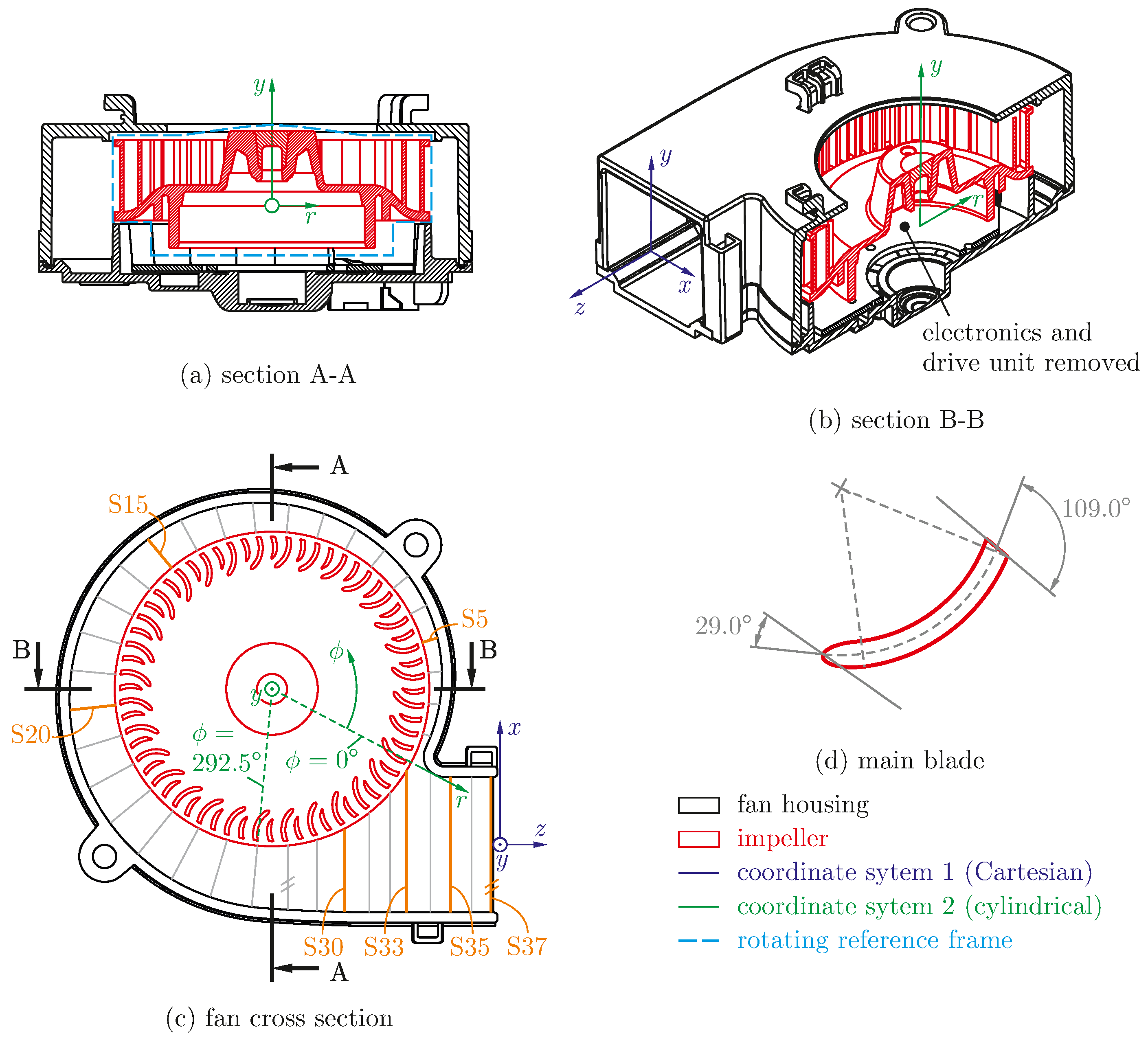
Figure 2.
Sections through the fan and rotor, showing the definition of the coordinate systems and evaluation surfaces.
Figure 2.
Sections through the fan and rotor, showing the definition of the coordinate systems and evaluation surfaces.
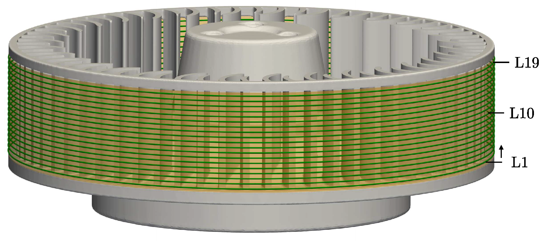
Figure 3.
Visualization of the nineteen evaluation lines located at the outer surface of the impeller.
Figure 3.
Visualization of the nineteen evaluation lines located at the outer surface of the impeller.
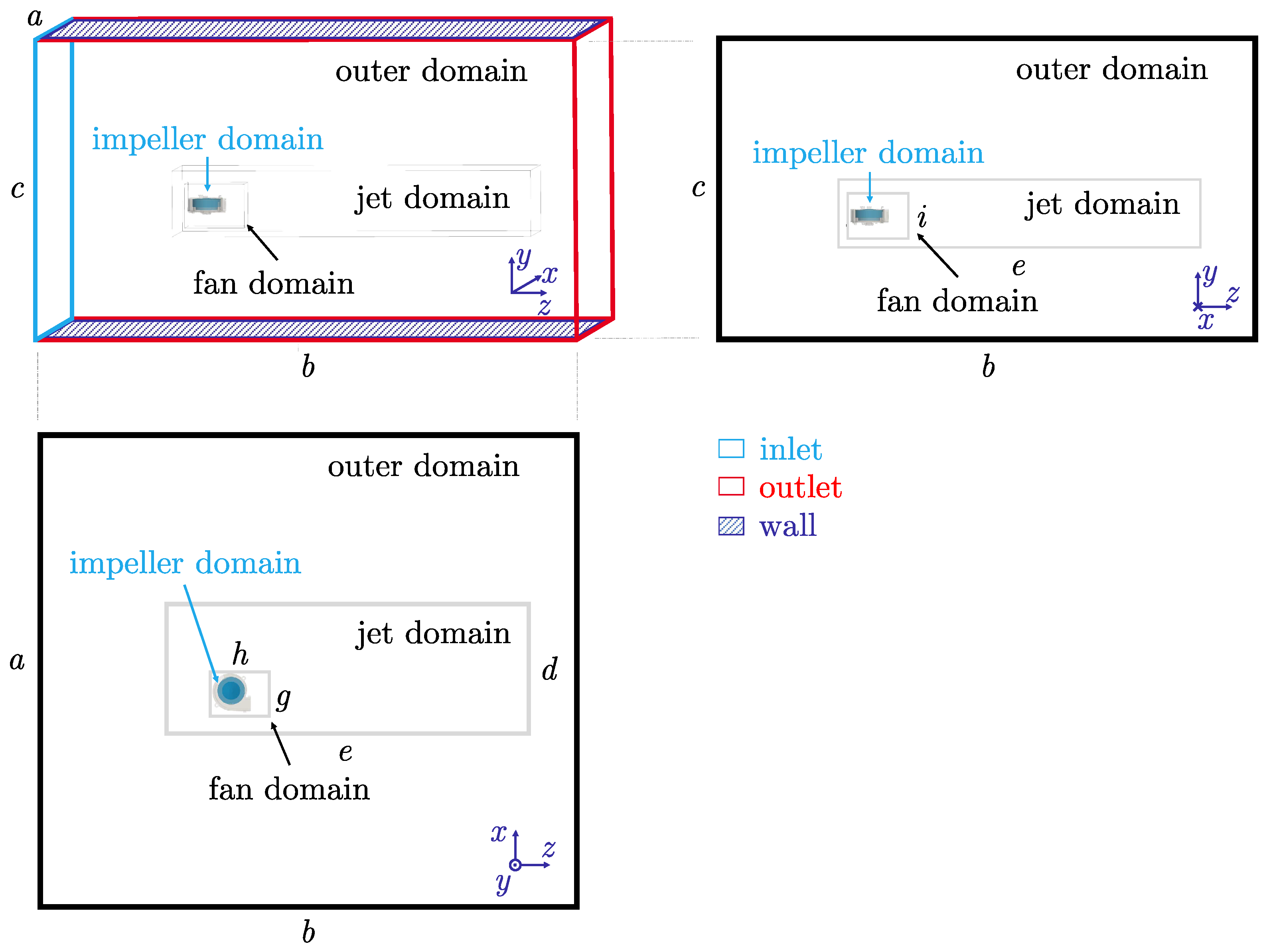
Figure 4.
Visualisation of the computational domains and its dimensions.
Figure 4.
Visualisation of the computational domains and its dimensions.
Figure 5.
Details of the generated fine mesh; the region colored in cyan in the lower two images indicates the rotating reference frame. (a) Fan wall mesh; looking into the fan via the outlet port. (b) Mesh detail for a cut-plane at , including outlet and volute nose. (c) Mesh detail for blade channel 27 for a cut-plane at .
Figure 6.
Convergence trend of the massflow weighted total pressure difference between fan inlet and the trend of the VFR at the impeller outlet; solid blue lines represent the simulation results, dashed black lines the power series expansion, and vertical dashed lines the 95% uncertainty estimates. (a) Total pressure difference between fan in- and outlet. (b) VFR at the impeller outlet.
Figure 7.
Mesh convergence study: Comparison of the normalized velocity magnitude results on a horizontal evaluation line over the fan outlet at (black dashed line) and visualization of the velocity contours of the fine mesh. (a) Evaluation line results. (b) Normalized velocity magnitude contours for the fine mesh.
Figure 8.
Height-averaged normalized velocity magnitude results at the rotor outlet of the steady, pseudo-transient and transient realizable k- simulations and the deviations with respect to the transient results. (a) Normalized velocity magnitude result. (b) Differences of the normalized velocity magnitude.
Figure 9.
Fraction of cell width to integral length scale L and the Kolmogorov length scale , respectively, obtained from URANS simulations. A cut-plane at is used to evaluate the results for the fine and very fine mesh, including the detailed situation between selected blade channels. Turbulent length scale estimation for the (a) fine mesh: fan cross section, (b) very fine mesh: fan cross-section, (c) fine mesh: blade channel detail, (d) very fine mesh: blade channel detail.
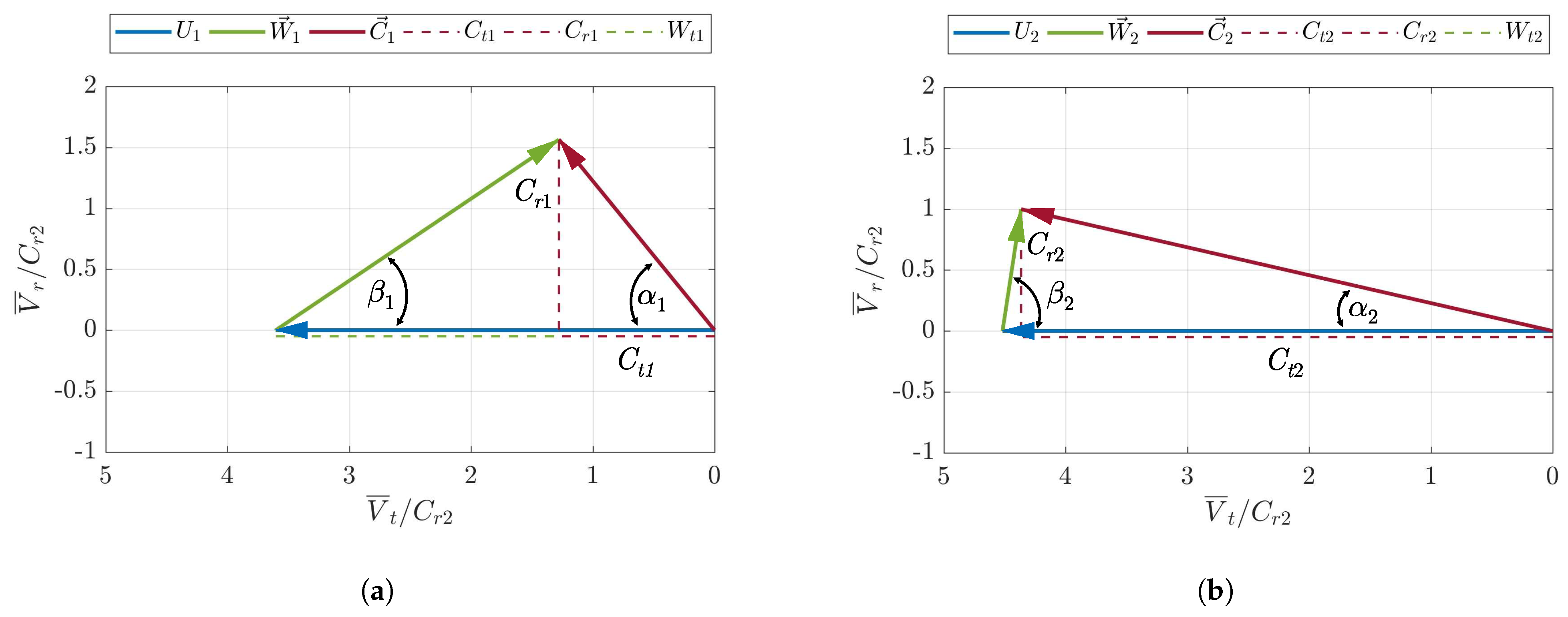
Figure 10.
Velocity triangles at the impeller inlet and outlet calculated from time- and spatially-averaged SAS results. Common nomenclature for velocity triangles is used here, absolute velocity, relative velocity, impeller tangential velocity. Indices 1 and 2 refer to the rotor inlet and outlet, respectively. (a) Velocity triangle at the impeller inlet. (b) Velocity triangle at the impeller outlet.
Figure 11.
Normalized time-averaged velocity magnitude results of the realizable k- simulation at the impeller outlet surface. The aspect ratio of the plot (impeller outlet height vs. outlet circumference) is increased by a factor of 8. Note: No moving average filter was applied.
Figure 11.
Normalized time-averaged velocity magnitude results of the realizable k- simulation at the impeller outlet surface. The aspect ratio of the plot (impeller outlet height vs. outlet circumference) is increased by a factor of 8. Note: No moving average filter was applied.
Figure 12.
Normalized time-averaged velocity magnitude results for the evaluation lines at the impeller outlet surface for the different turbulence models; bottom (blue, L1), mid (green, L10), top (red, L19), others (grey).
Figure 12.
Normalized time-averaged velocity magnitude results for the evaluation lines at the impeller outlet surface for the different turbulence models; bottom (blue, L1), mid (green, L10), top (red, L19), others (grey).
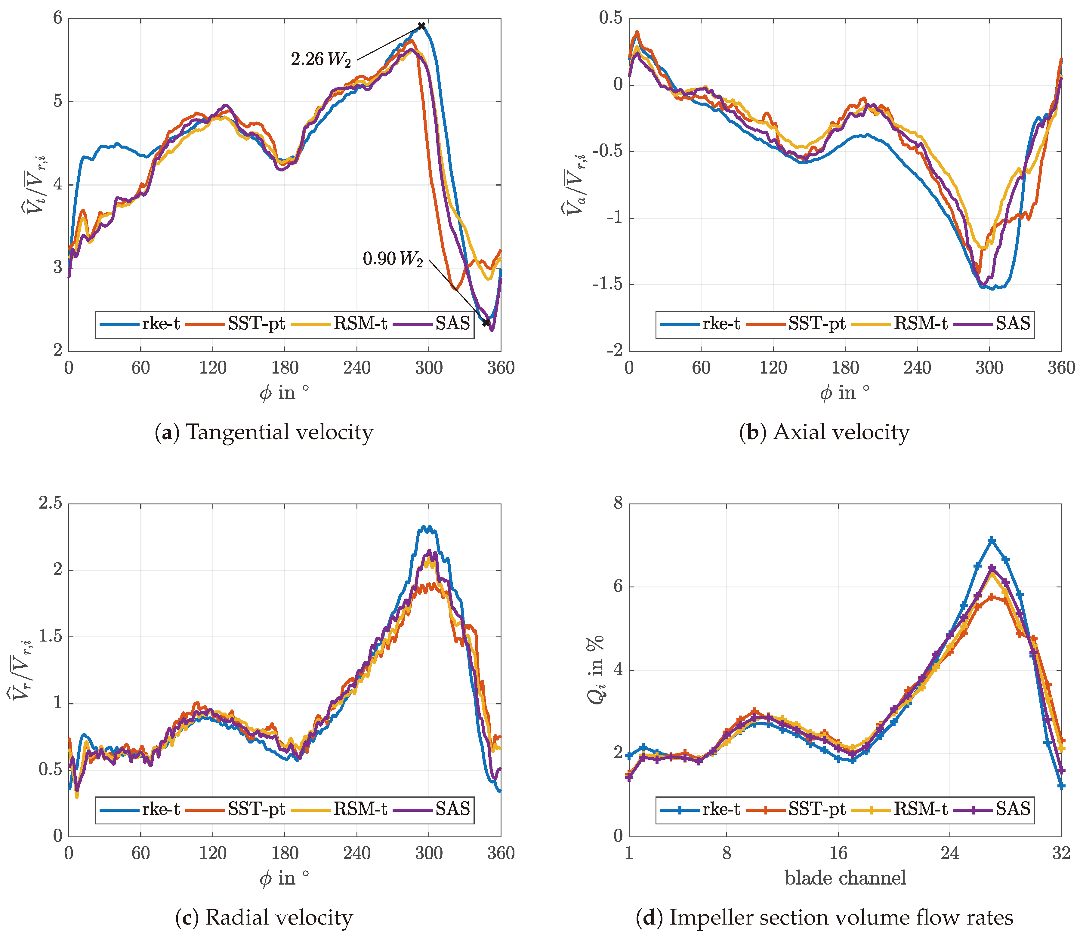
Figure 13.
Time-averaged normalized tangential, axial and radial velocity averaged over all 19 evaluation lines at the impeller outlet as well as the blade channel volume flow rates for the different turbulence models.
Figure 13.
Time-averaged normalized tangential, axial and radial velocity averaged over all 19 evaluation lines at the impeller outlet as well as the blade channel volume flow rates for the different turbulence models.
Figure 14.
Time-averaged normalized velocity magnitude results for six different evaluation surfaces of the fan volute and the different turbulence models. (a) includes a sketch of the cross-section of the fan for orientation purposes: ➀ …upper impeller ring, ➁ …blade channel, ➂ …impeller base plate, ➃ …lower impeller gap, ➄ …lower volute extension. Velocity magnitude for evaluation surface (a) S5, (b) S15, (c) S20, (d) S30, (e) S33, (f) S35.
Figure 15.
Time-averaged normalized axial and radial velocity results for three different evaluation surfaces of the fan volute and the different turbulence models. (a) Axial velocity for evaluation surface S20. (b) Radial velocity for evaluation surface S20. (c) Axial velocity for evaluation surface S30. (d) Radial velocity for evaluation surface S30. (e) Axial velocity for evaluation surface S33. (f) Radial velocity for evaluation surface S33.
Figure 16.
Normalized relative velocity magnitude and normalized static pressure results for a selected time step at an evaluation surface at , slightly above the middle height of the impeller outlet. Note: The white dashed line indicates the MRF border. Overlaid LIC lines: (a) shows LIC lines calculated from the relative velocity field, (b) from the absolute velocity field.
Figure 17.
Normalized relative velocity magnitude results for selected blade channels at an evaluation surface inside the fan at , slightly above the middle height of the impeller outlet.
Figure 17.
Normalized relative velocity magnitude results for selected blade channels at an evaluation surface inside the fan at , slightly above the middle height of the impeller outlet.
Figure 18.
Time-averaged normalized velocity magnitude, x-, y- and z- velocity results at the fan outlet (S37) for the different turbulence models.
Figure 18.
Time-averaged normalized velocity magnitude, x-, y- and z- velocity results at the fan outlet (S37) for the different turbulence models.
Figure 19.
Normalized turbulent kinetic energy of all turbulence models for selected time steps at an evaluation surface at , slightly above the middle height of the impeller outlet.
Figure 19.
Normalized turbulent kinetic energy of all turbulence models for selected time steps at an evaluation surface at , slightly above the middle height of the impeller outlet.
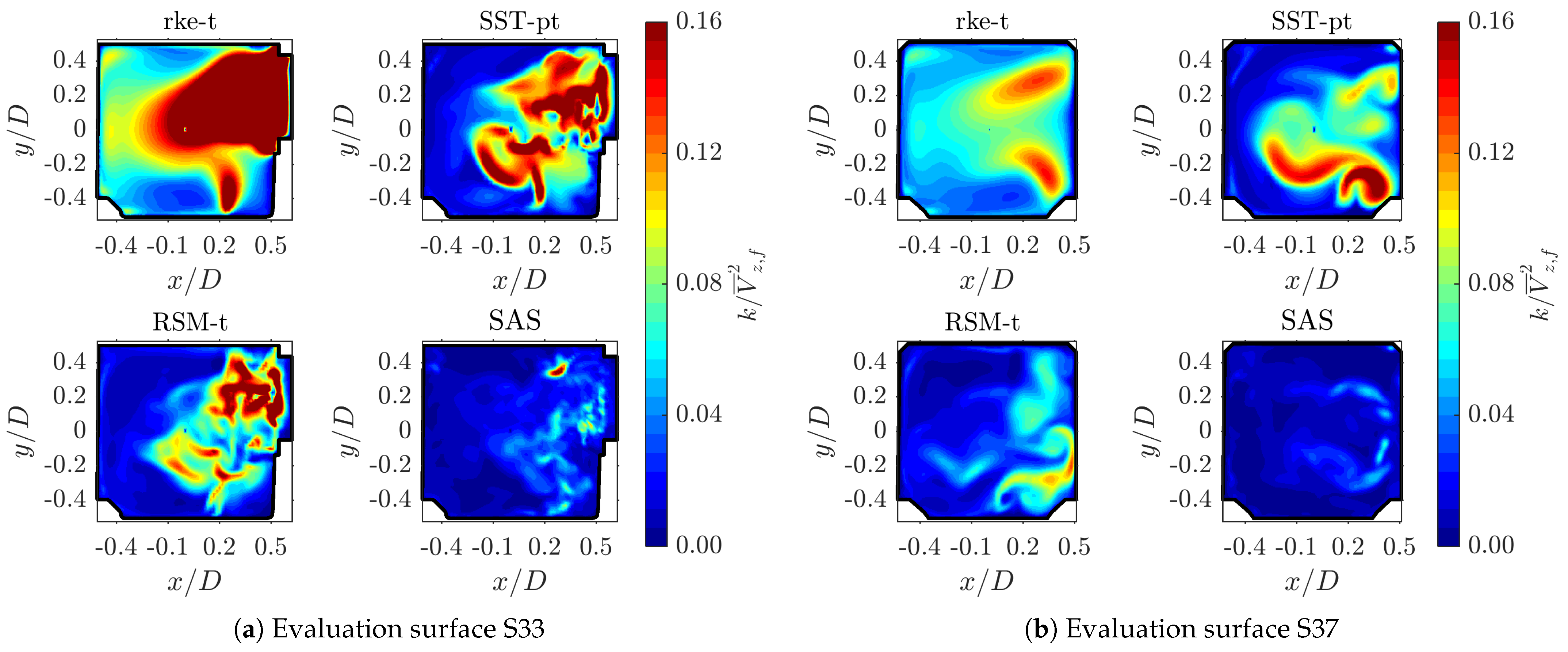
Figure 20.
Normalized turbulent kinetic energy at the evaluation surfaces S33 and S37 (fan outlet) for the different turbulence models.
Figure 20.
Normalized turbulent kinetic energy at the evaluation surfaces S33 and S37 (fan outlet) for the different turbulence models.
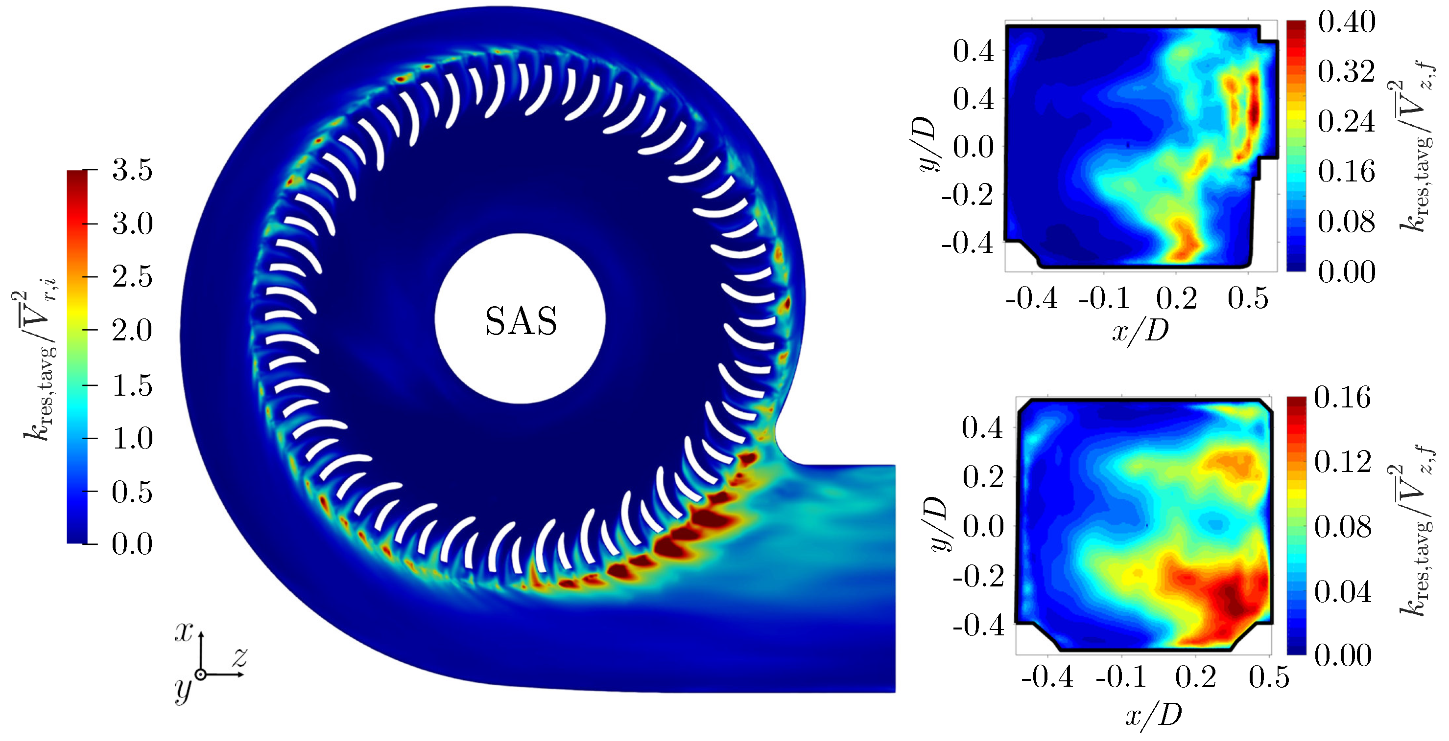
Figure 21.
Normalized time-averaged resolved turbulent kinetic energy results of the SAS model at an evaluation surface at and at the evaluation surfaces S33 and S37 (fan outlet).
Figure 21.
Normalized time-averaged resolved turbulent kinetic energy results of the SAS model at an evaluation surface at and at the evaluation surfaces S33 and S37 (fan outlet).
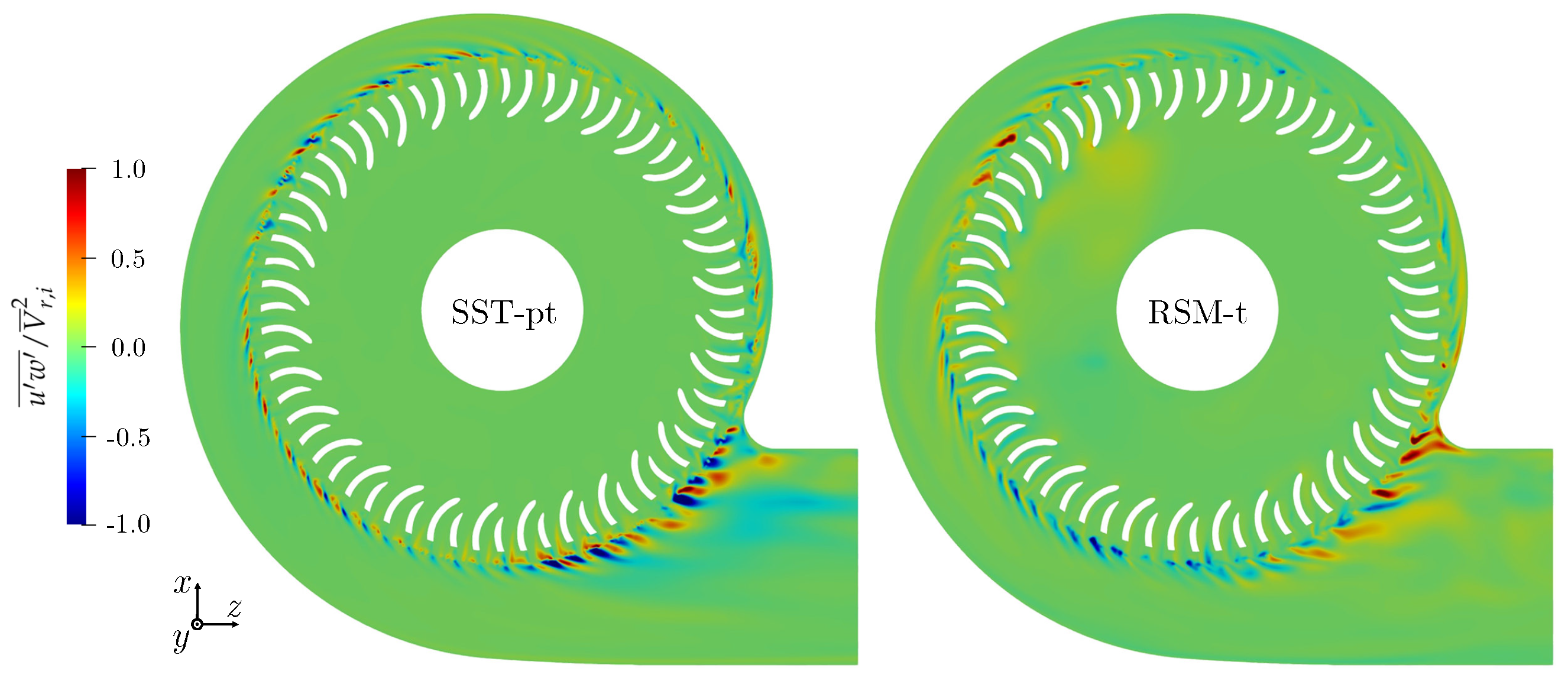
Figure 22.
Comparison of normalized Reynolds stress results of the SST k- and RSM simulation for a selected time step at an evaluation surface at .
Figure 22.
Comparison of normalized Reynolds stress results of the SST k- and RSM simulation for a selected time step at an evaluation surface at .
Figure 23.
Comparison of normalized Reynolds stress results of the SST k- and RSM simulation for a selected time step at an evaluation surface at .
Figure 23.
Comparison of normalized Reynolds stress results of the SST k- and RSM simulation for a selected time step at an evaluation surface at .
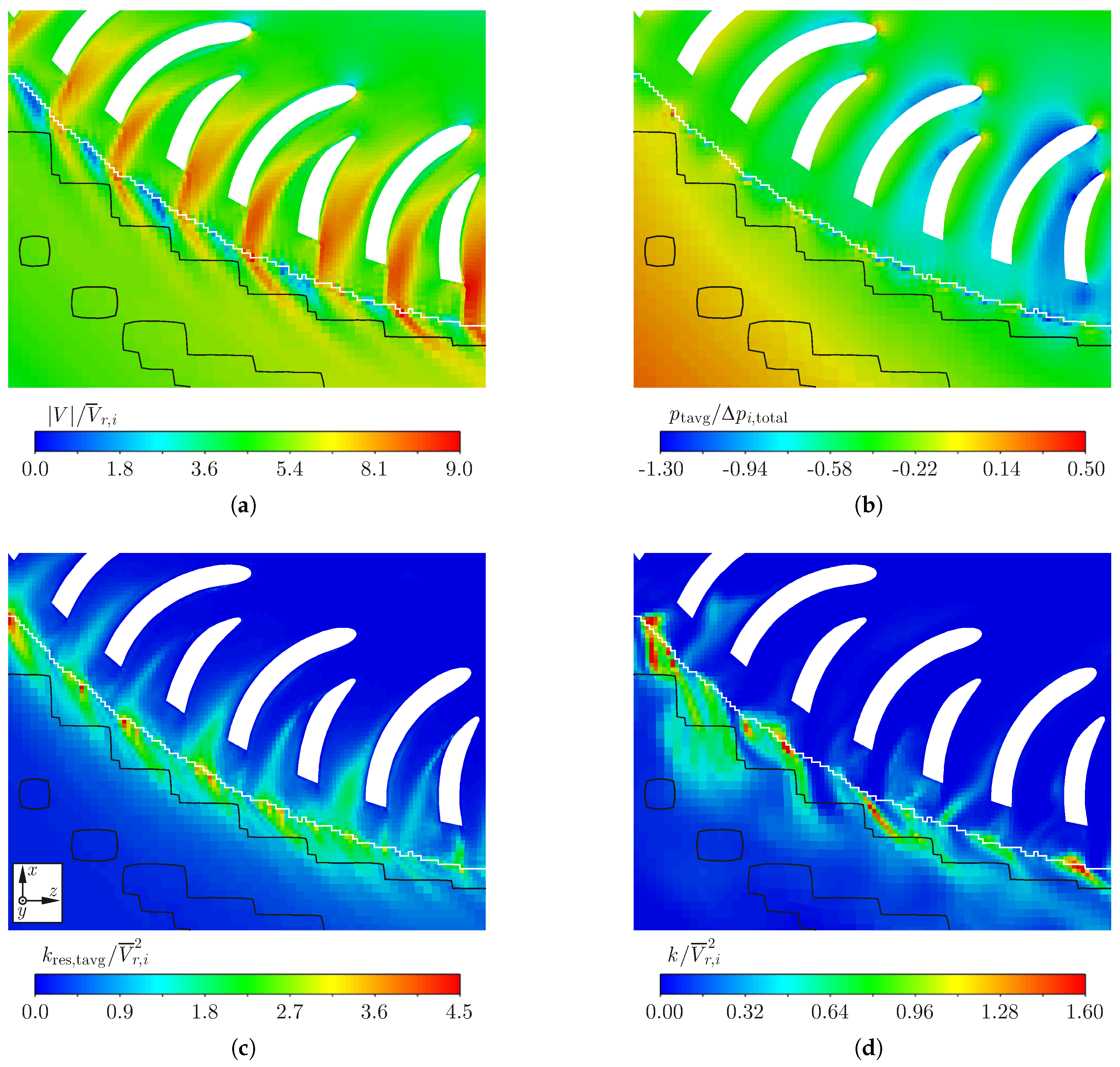
Figure 24.
Cell-value contours of SAS simulation results for velocity, pressure and turbulent kinetic energy; details in the vicinity of blade channels 24 and 25; black lines indicate borders of regions with uniform mesh resolution, the white line indicates the boundary of the rotating reference frame. (a) normalized time-averaged velocity magnitude. (b) normalized time-averaged static pressure. (c) normalized time-averaged resolved turbulent kinetic energy. (d) normalized modeled turbulent kinetic energy.
Figure 25.
Cell-value contours of SAS simulation results for different turbulence quantities; details in the vicinity of blade channels 24 and 25; black lines indicate borders of regions with uniform mesh resolution, the white line indicates the boundary of the rotating reference frame. (a) normalized modeled specific dissipation rate. (b) normalized time-averaged turbulent viscosity ratio. (c) normalized time-averaged resolved -stress. (d) normalized time-averaged modeled -stress.
Figure 26.
Time-averaged normalized and velocity contours at the fan outlet slightly downstream of evaluation surface S37 at for the CTA measurements and the different turbulence models. Note: The white lines indicate the fan outlet edges.
Figure 26.
Time-averaged normalized and velocity contours at the fan outlet slightly downstream of evaluation surface S37 at for the CTA measurements and the different turbulence models. Note: The white lines indicate the fan outlet edges.
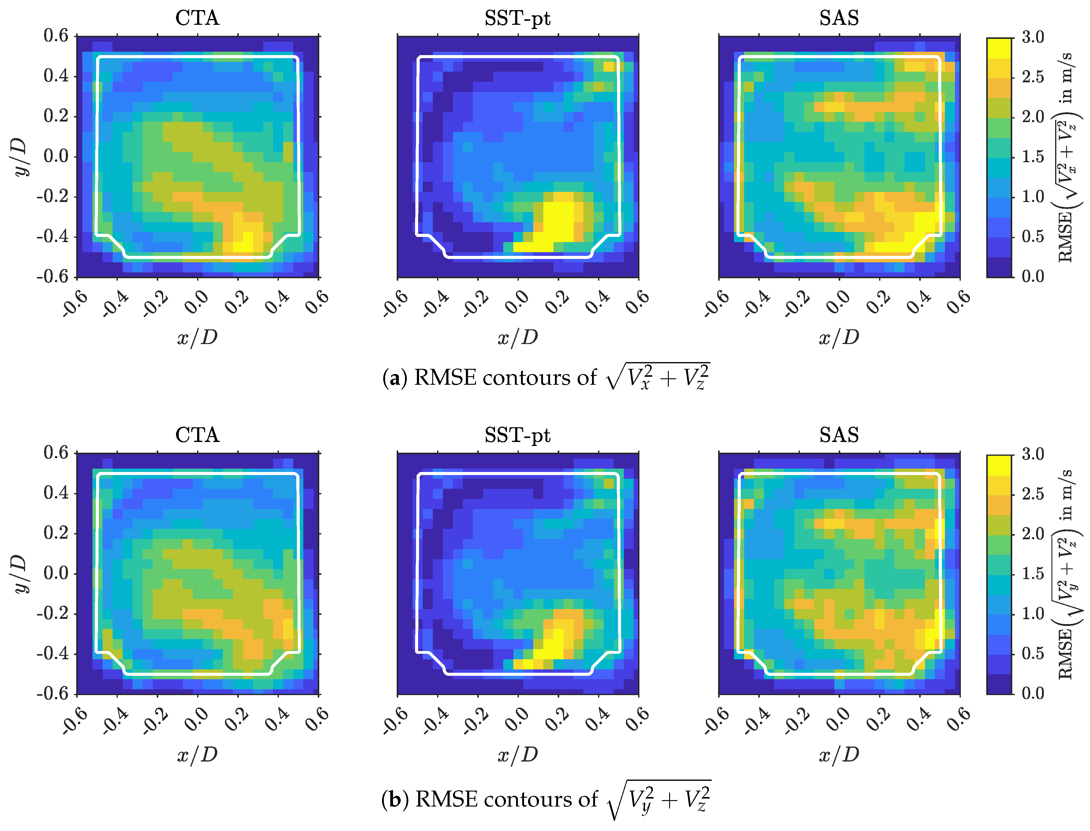
Figure 27.
RMSE values of and at the fan outlet slightly downstream of evaluation surface S37 at for the CTA measurements and selected turbulence models. Note: The white lines indicate the fan outlet edges.
Figure 27.
RMSE values of and at the fan outlet slightly downstream of evaluation surface S37 at for the CTA measurements and selected turbulence models. Note: The white lines indicate the fan outlet edges.
Figure 28.
Time-averaged normalized velocity contours of various -planes showing the development of the jet’s cross section with increasing outlet distance. Note: Red lines indicate FWHM.
Figure 28.
Time-averaged normalized velocity contours of various -planes showing the development of the jet’s cross section with increasing outlet distance. Note: Red lines indicate FWHM.
Table 1.
Specifications of fan MSG L775.
Table 1.
Specifications of fan MSG L775.
| Fan Casing |
|---|
| outer dimensions | 65.3 mm × 64.5 mm × 23.5 mm |
| outlet dimension | | 20 mm × 20 mm |
| inlet diameter | |
31 mm
|
| characteristic length | D | 20 mm |
| fan outlet area | |
400 mm2 |
| Impeller |
| main blade outer diameter | |
45.0 mm
|
| main blade inner diameter | |
35.9 mm
|
| splitter blade inner diameter | |
38.5 mm
|
| impeller height | |
9.0 mm
|
| number of blade pairs | | 32 |
| impeller outlet area | |
1417 mm2 |
| blade sweep | forward-curved |
| Nominal Fan Parameters |
| nominal supply voltage | |
12 V
|
| nominal supply current | |
135 mA
|
| nominal impeller speed | | |
| nominal VFR | | |
| nominal total fan pressure | | |
| nominal overall fan efficiency | | 12% |
| measured supply voltage | |
13.5 V
|
| measured supply current | |
187.2 m
|
| measured impeller speed at
| |
5033 rpm
|
| measured VFR | | |
| measured static fan pressure | |
0 Pa
|
Table 2.
Mesh domain dimensions.
Table 2.
Mesh domain dimensions.
| Notation | Variables | Dimension | Normalized Dimension |
|---|
| outer domain | |
| |
| jet domain | |
| |
| fan domain | |
| |
Table 3.
Material properties of the fluid air.
Table 3.
Material properties of the fluid air.
| Variable | Notation | Result |
|---|
| Density | | |
| Dynamic viscosity | | 1.7894 × 10⁻⁵ |
Table 4.
Mesh sizes, maximum cell sizes and average values of the created meshes.
Table 4.
Mesh sizes, maximum cell sizes and average values of the created meshes.
| Notation | Very Rough | Rough | Fine | Very Fine |
|---|
| Number of cells | 5 × 10⁶ | 9 × 10⁶ | 21 × 106 | 36 × 106 |
| Cell size outer domain | 15 mm | 12 mm | 8 mm | 6 mm |
| Cell size jet dom. |
3.75 mm
|
3.0 mm
|
2.0 mm
|
1.5 mm
|
| Cell size impeller dom. |
0.938 mm
|
0.75 mm
|
0.5 mm
|
0.375 mm
|
| Cell size blade section |
0.469 mm
|
0.188 mm
|
0.125 mm
|
0.094 mm
|
| average fan | 3.1 | 2.5 | 1.9 | 1.4 |
Table 5.
Comparison of fan performance results obtained with the four different turbulence models.
Table 5.
Comparison of fan performance results obtained with the four different turbulence models.
| Turbulence Model | (Pa) | () | () | |
|---|
| rke-t | 58.0 | 12.4 | 8.69 | |
| SST-pt | 60.1 | 11.6 | 8.17 | |
| RSM-t | 52.8 | 11.8 | 8.30 | |
| SAS | 56.3 | 12.2 | 8.59 | |
Table 6.
Comparison of dimensionless fan performance parameters obtained with the four different turbulence models.
Table 6.
Comparison of dimensionless fan performance parameters obtained with the four different turbulence models.
| Turbulence Model | | | | |
|---|
| rke-t | 0.184 | 2.142 | 0.242 | 2.824 |
| SST-pt | 0.173 | 2.220 | 0.229 | 2.935 |
| RSM-t | 0.175 | 1.950 | 0.254 | 2.821 |
| SAS | 0.181 | 2.082 | 0.246 | 2.820 |
Table 7.
Comparison of impeller performance results obtained with the four different turbulence models.
Table 7.
Comparison of impeller performance results obtained with the four different turbulence models.
| Turbulence Model | (Pa) | (Pa) | (Pa) | (Pa) | (Pa) | () | () |
|---|
| rke-t | 128.7 | 136.1 | 30.9 | 74.5 | 30.7 | 13.3 | 2.61 |
| SST-pt | 137.8 | 120.5 | 30.9 | 61.2 | 28.4 | 12.7 | 2.48 |
| RSM-t | 125.0 | 124.7 | 30.9 | 64.6 | 29.2 | 12.9 | 2.52 |
| SAS | 126.5 | 125.9 | 30.9 | 66.5 | 28.5 | 13.3 | 2.61 |
Table 8.
Comparison of fan efficiency results obtained with the four different turbulence models.
Table 8.
Comparison of fan efficiency results obtained with the four different turbulence models.
| Turbulence Model | (%) | (%) | (%) | (%) | (%) |
|---|
| rke-t | 7.9 | 29.5 | 63.7 | 45.0 | 93.1 |
| SST-pt | 7.6 | 26.9 | 71.2 | 43.0 | 92.0 |
| RSM-t | 6.9 | 27.2 | 65.1 | 42.2 | 92.0 |
| SAS | 7.6 | 29.0 | 63.8 | 44.6 | 92.0 |
Table 9.
Comparison of the velocities and angles of the velocity triangles at the impeller inlet for the different turbulence models.
Table 9.
Comparison of the velocities and angles of the velocity triangles at the impeller inlet for the different turbulence models.
| Turbulence Model | (°) | (°) | () | () | () |
|---|
| rke-t | 53.3 | 32.9 | 9.40 | 7.55 | 5.12 |
| SST-pt | 50.3 | 31.8 | 9.40 | 7.30 | 5.00 |
| RSM-t | 51.2 | 32.2 | 9.40 | 7.37 | 5.05 |
| SAS | 50.8 | 33.9 | 9.40 | 7.31 | 5.27 |
Table 10.
Comparison of the velocities and angles of the velocity triangles at the impeller outlet for the different turbulence models.
Table 10.
Comparison of the velocities and angles of the velocity triangles at the impeller outlet for the different turbulence models.
| Turbulence Model | (°) | (°) | () | () | () |
|---|
| rke-t | 12.4 | 88.0 | 11.78 | 2.61 | 12.15 |
| SST-pt | 12.8 | 70.4 | 11.78 | 2.63 | 11.18 |
| RSM-t | 12.7 | 76.0 | 11.78 | 2.60 | 11.44 |
| SAS | 12.9 | 81.3 | 11.78 | 2.64 | 11.68 |
Table 11.
Comparison of the volume flow rates derived from CTA measurements and the conducted simulations.
Table 11.
Comparison of the volume flow rates derived from CTA measurements and the conducted simulations.
| Source |
() | () |
() |
|---|
| rke-t | 13.2 | 13.0 | 12.9 |
| SST-pt | 12.3 | 12.1 | 11.9 |
| RSM-t | 12.4 | 12.2 | 12.1 |
| SAS | 13.0 | 12.6 | 12.5 |
| Measurements (CTA) | 13.4 | 12.9 | - |


