

A Deep Learning Approach to Improve the Control of Dynamic Wireless Power Transfer Systems

 ,
,  ,
,  and
and 
Abstract
:1. Introduction
2. WPTS Model
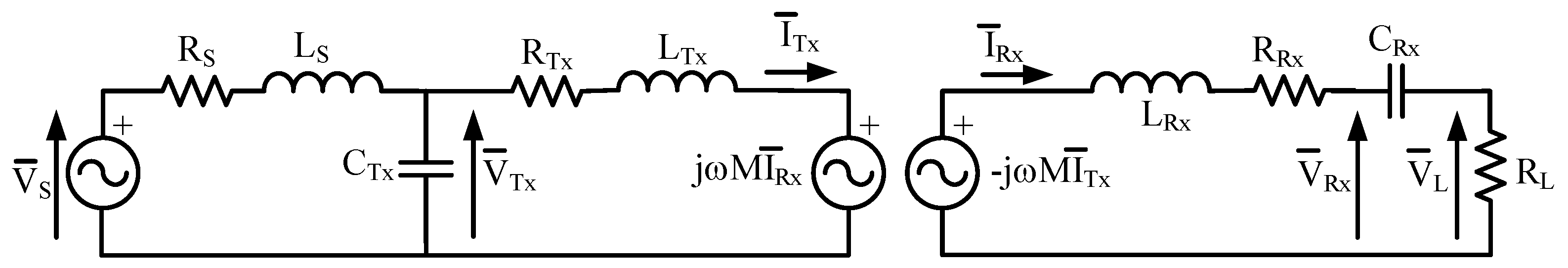
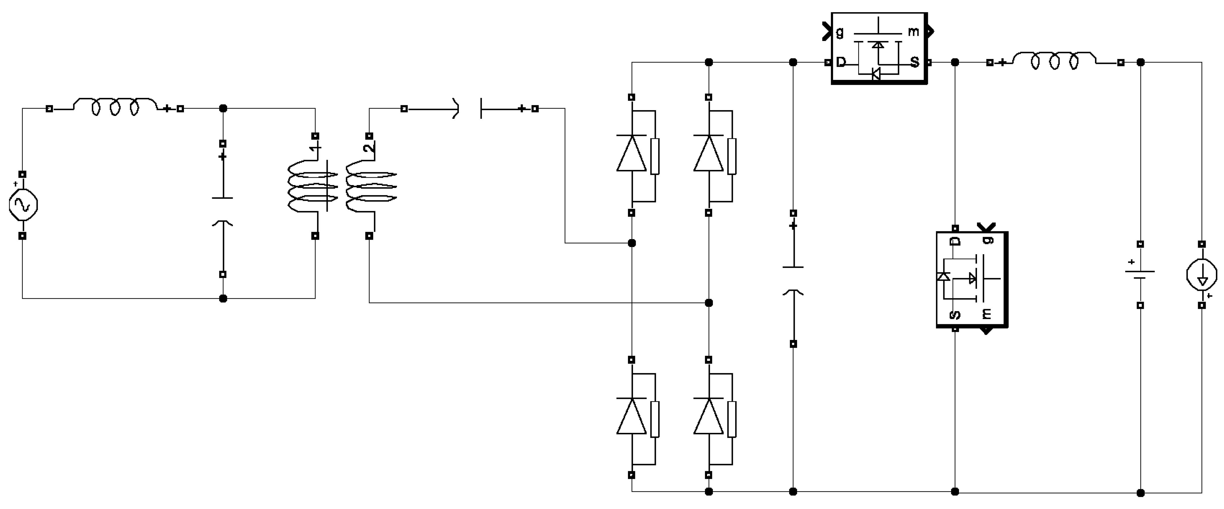
2.1. Lumped Parameter WPTS Model
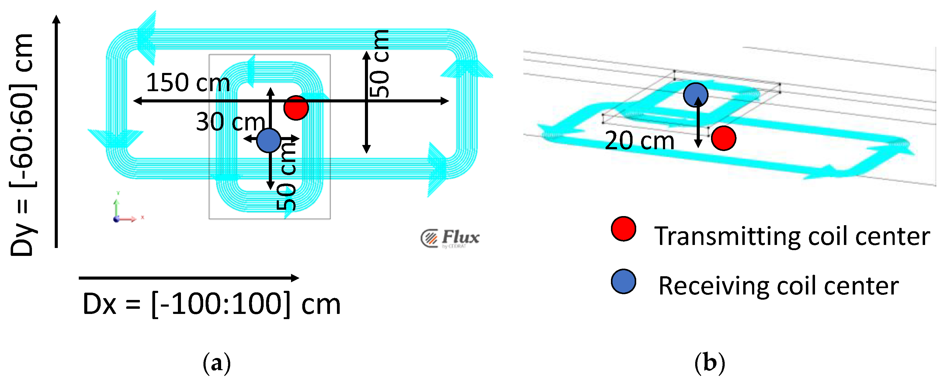
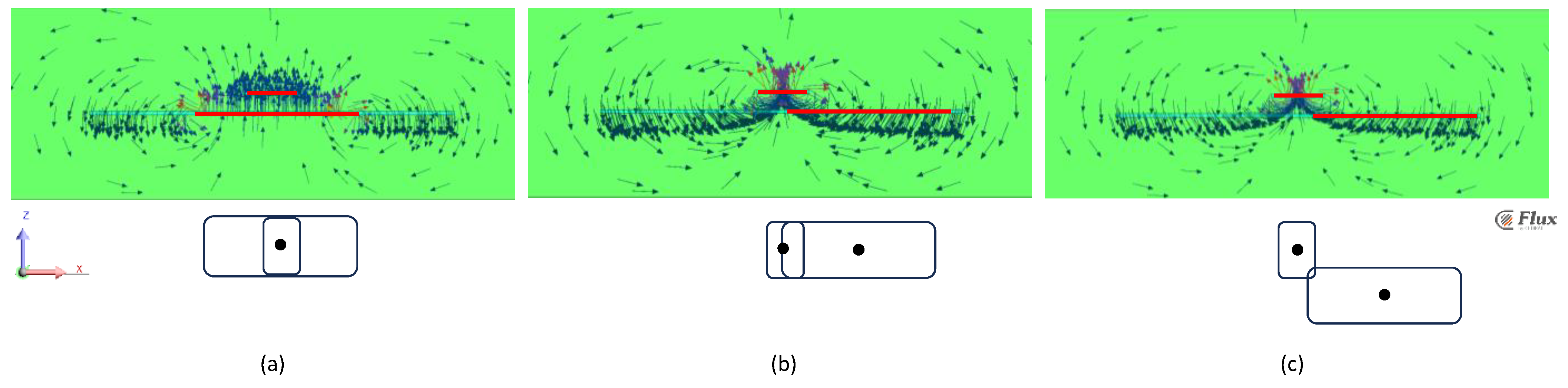
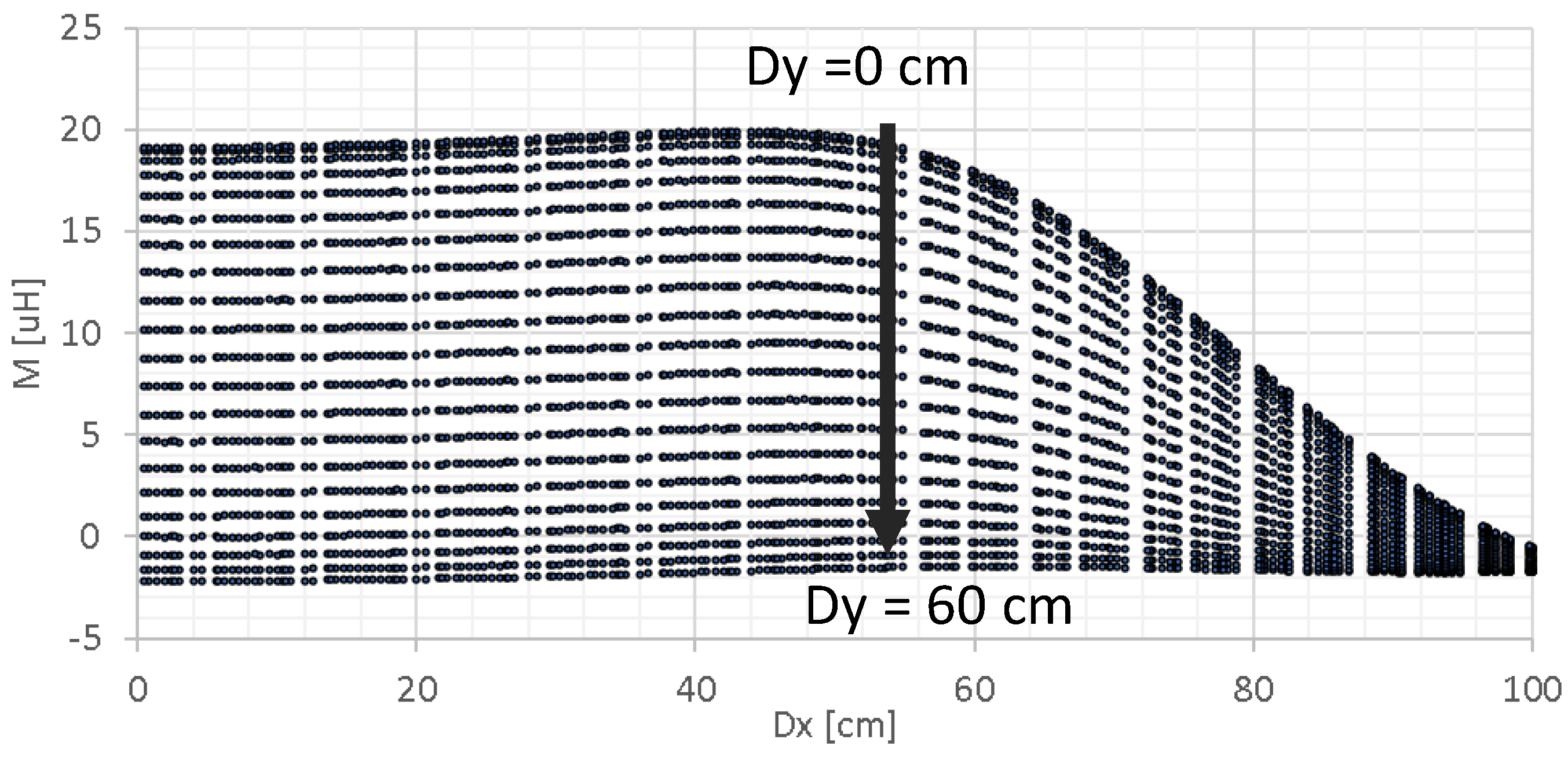
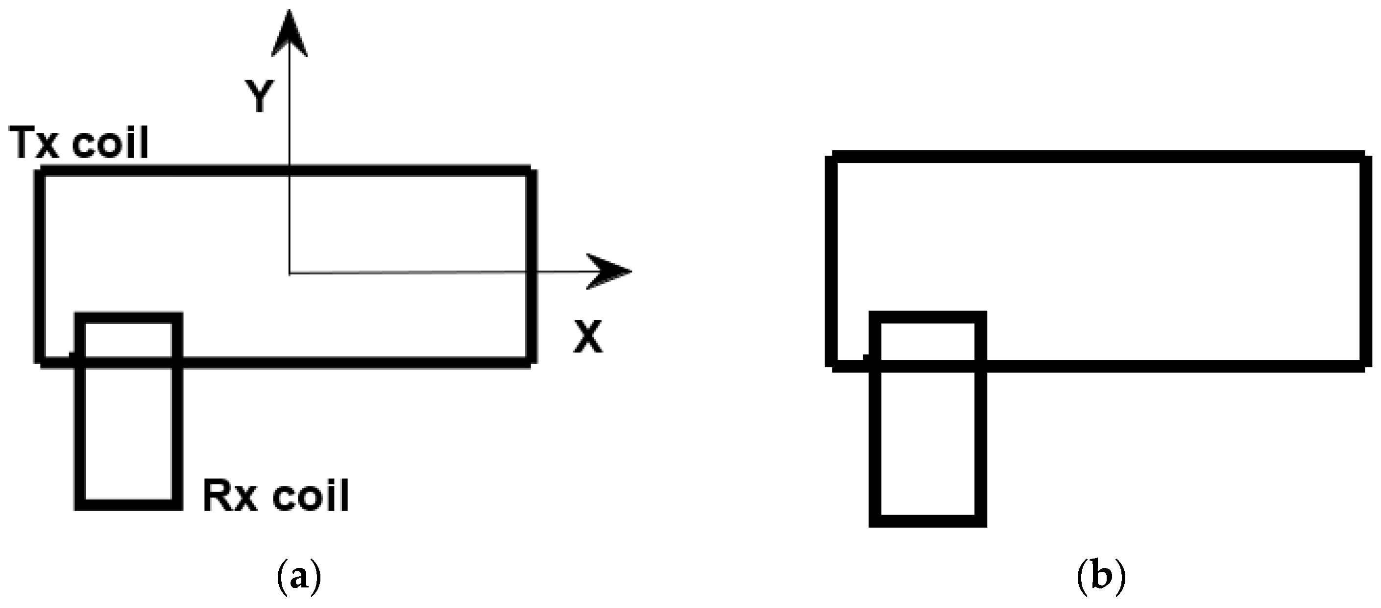
2.2. Field Model of WPTS for Database Creation: Finite Element Analysis
2.3. CNN-Based Approach
2.4. Control Strategy
3. Results
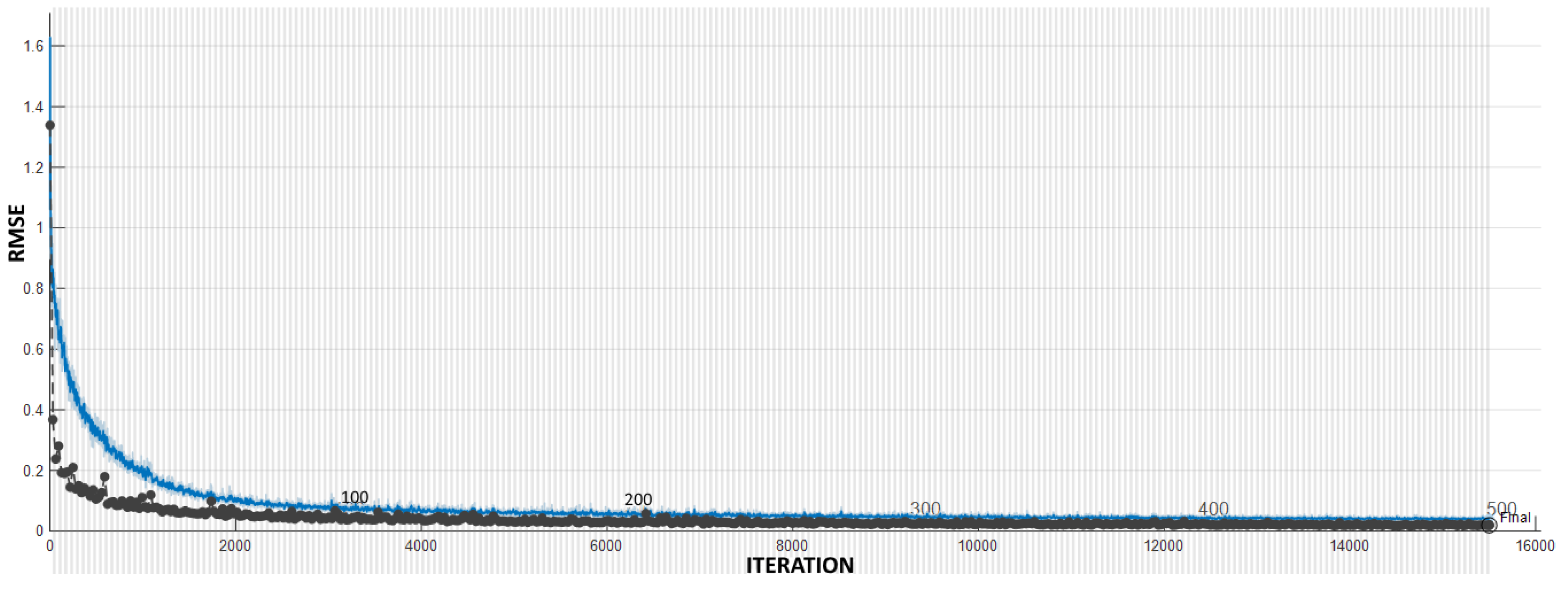
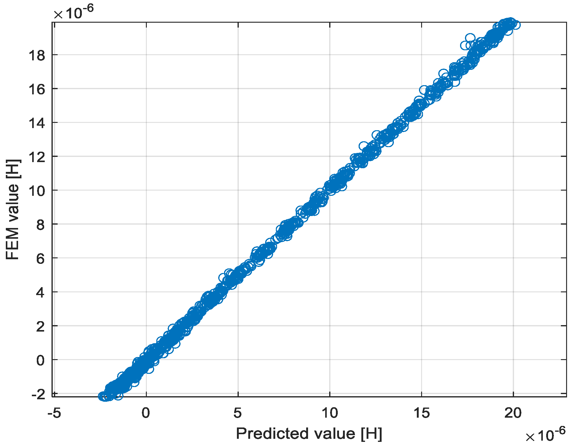
3.1. CNN Training
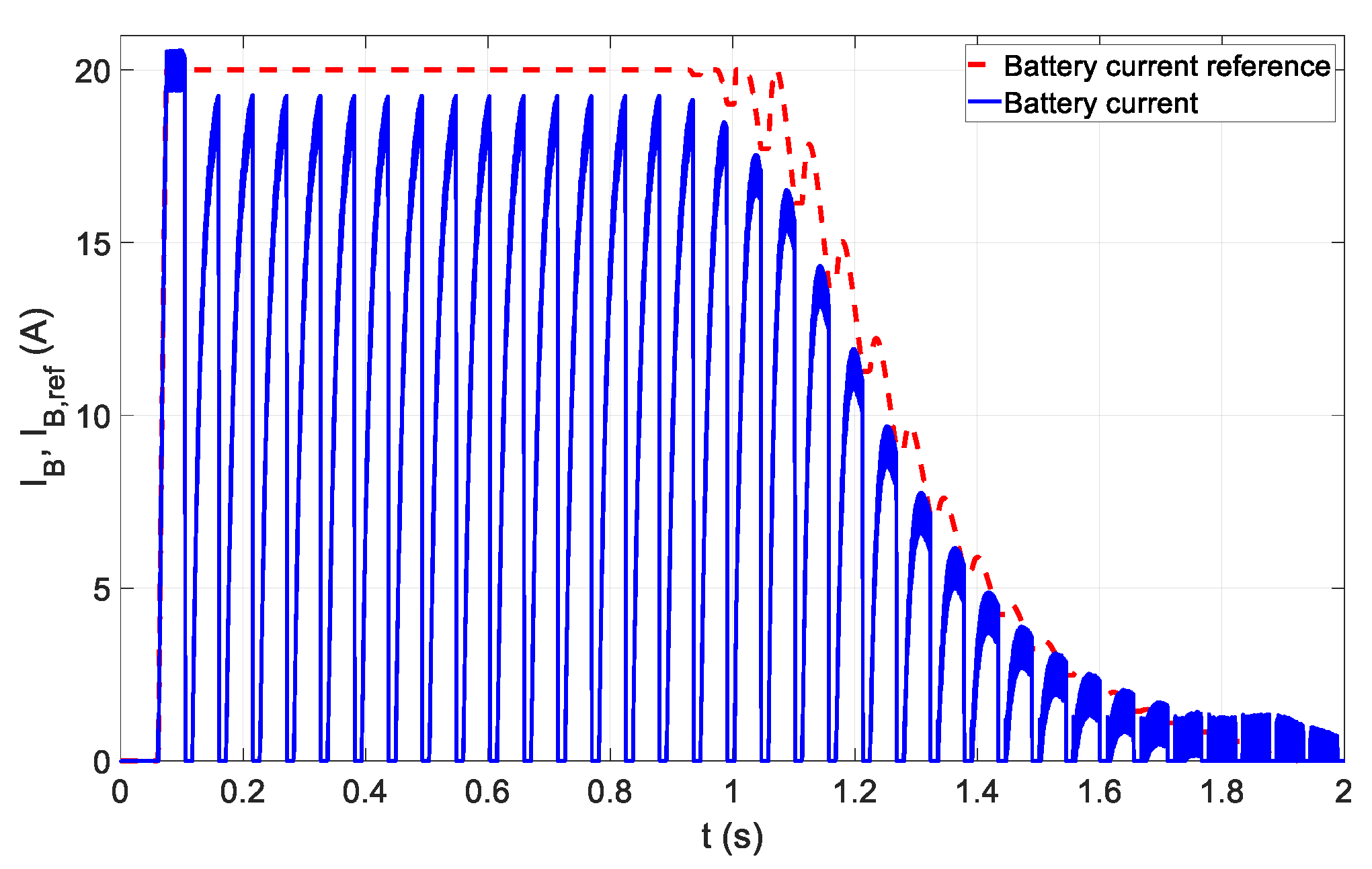
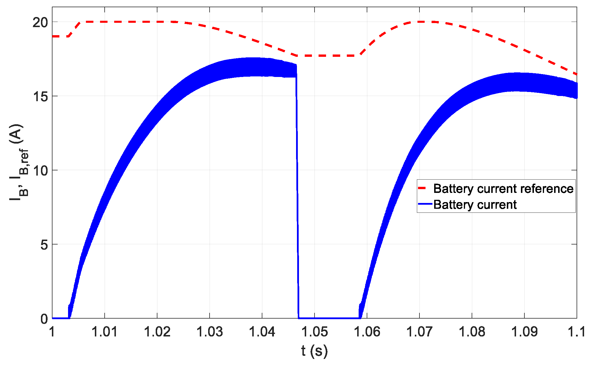
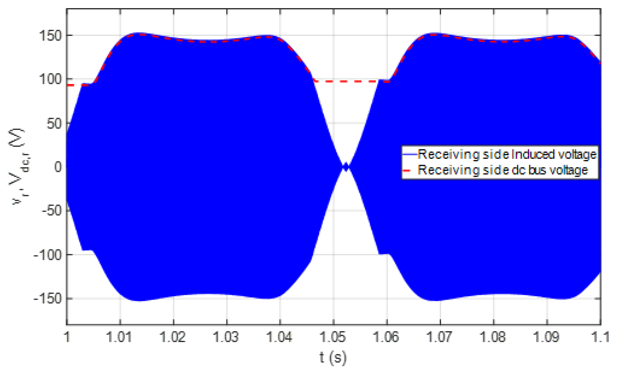
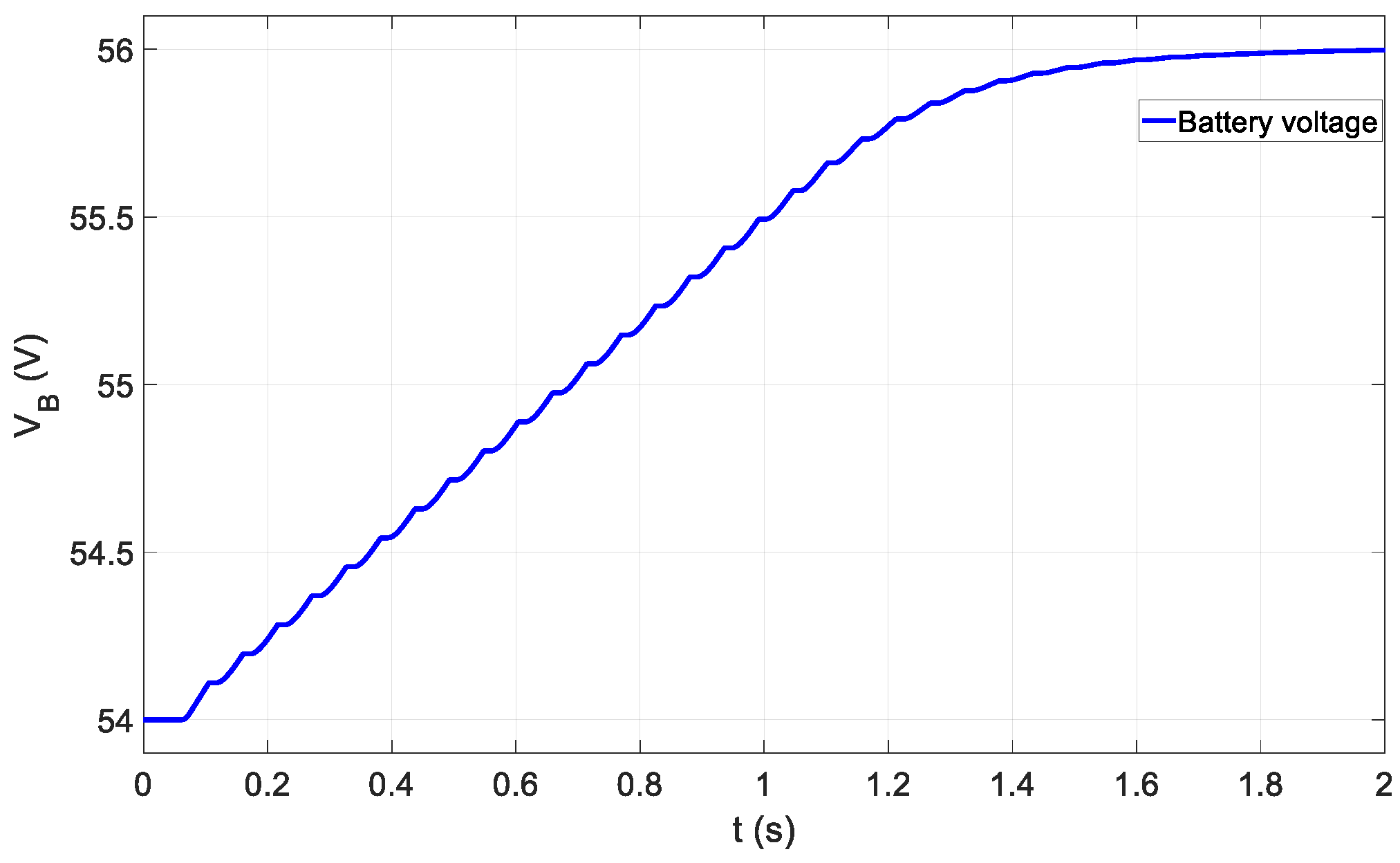
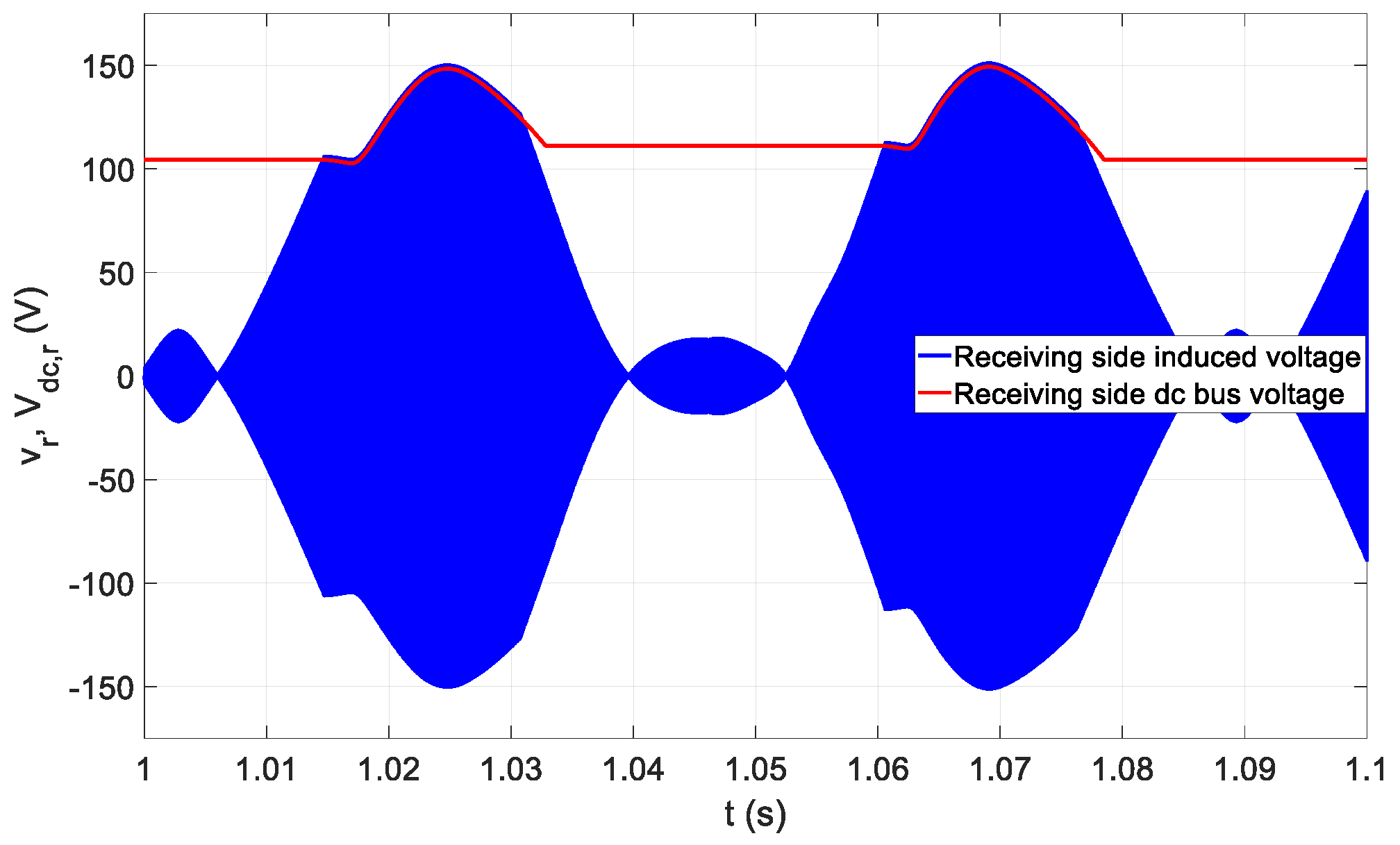
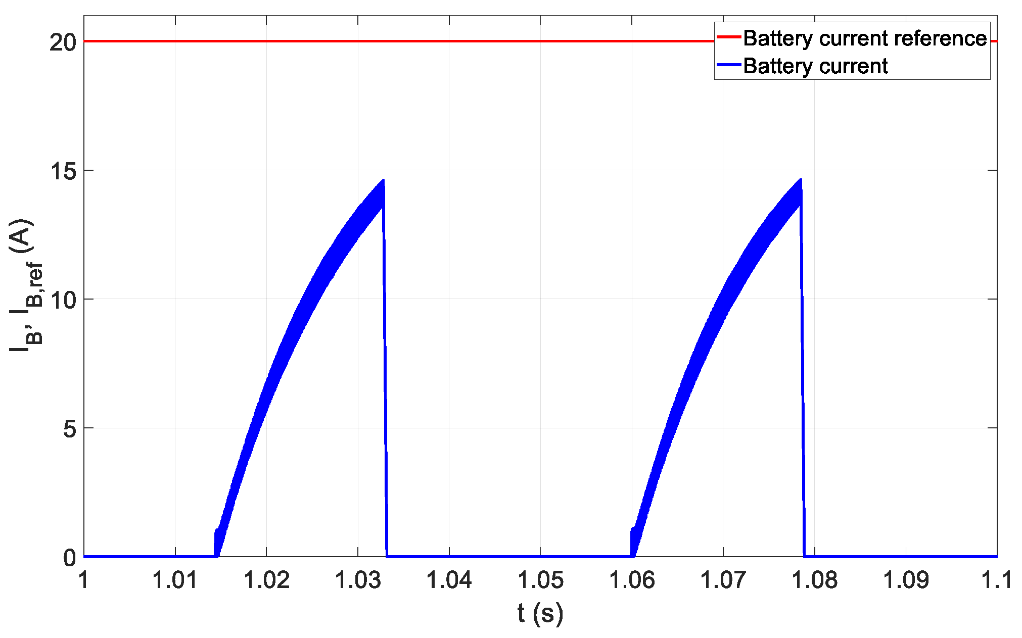
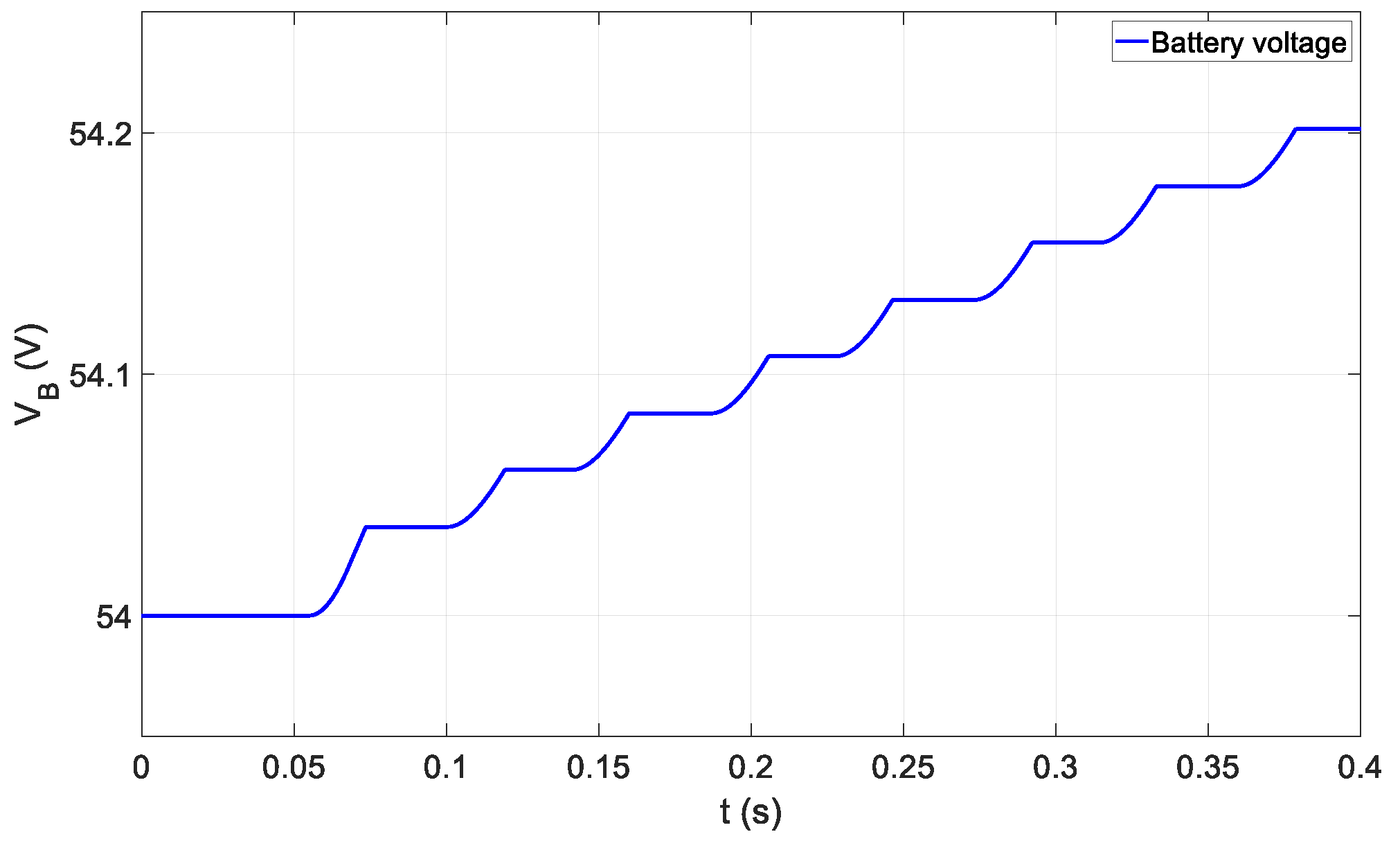
3.2. Battery Charging
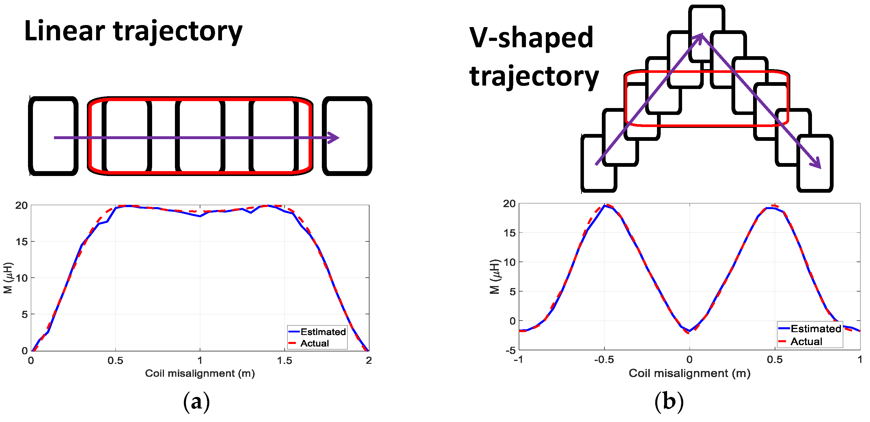
3.3. Linear Trajectory
3.4. V-Shaped Trajectory
4. Conclusions
Author Contributions
Funding
Data Availability Statement
Conflicts of Interest
References
- Cirimele, V.; Diana, M.; Freschi, F.; Mitolo, M. Inductive Power Transfer for Automotive Applications: State-of-the-Art and Future Trends. IEEE Trans. Ind. Appl. 2018, 54, 4069–4079. [Google Scholar] [CrossRef]
- Choi, S.Y.; Gu, B.W.; Jeong, S.Y.; Rim, C.T. Advances in Wireless Power Transfer Systems for Roadway-Powered Electric Vehicles. IEEE J. Emerg. Sel. Top. Power Electron. 2015, 3, 18–36. [Google Scholar] [CrossRef]
- Triviño, A.; González-González, J.M.; Aguado, J.A. Wireless Power Transfer Technologies Applied to Electric Vehicles: A Review. Energies 2021, 14, 1547. [Google Scholar] [CrossRef]
- Kindl, V.; Frivaldsky, M.; Zavrel, M.; Pavelek, M. Generalized Design Approach on Industrial Wireless Chargers. Energies 2020, 13, 2697. [Google Scholar] [CrossRef]
- Tan, L.; Zhang, M.; Wang, S.; Pan, S.; Zhang, Z.; Li, J.; Huang, X. The Design and Optimization of a Wireless Power Transfer System Allowing Random Access for Multiple Loads. Energies 2019, 12, 1017. [Google Scholar] [CrossRef]
- Feng, H.; Tavakoli, R.; Onar, O.C.; Pantic, Z. Advances in High-Power Wireless Charging Systems: Overview and Design Considerations. IEEE Trans. Transp. Electrific. 2020, 6, 886–919. [Google Scholar] [CrossRef]
- Liang, C.; Yang, G.; Yuan, F.; Huang, X.; Sun, Y.; Li, J.; Song, K. Modeling and Analysis of Thermal Characteristics of Magnetic Coupler for Wireless Electric Vehicle Charging System. IEEE Access 2020, 8, 173177–173185. [Google Scholar] [CrossRef]
- Li, S.; Mi, C.C. Wireless Power Transfer for Electric Vehicle Applications. IEEE J. Emerg. Sel. Top. Power Electron. 2015, 3, 4–17. [Google Scholar] [CrossRef]
- Yakala, R.K.; Pramanick, S.; Nayak, D.P.; Kumar, M. Optimization of Circular Coil Design for Wireless Power Transfer System in Electric Vehicle Battery Charging Applications. Trans Indian Natl. Acad. Eng. 2021, 6, 765–774. [Google Scholar] [CrossRef]
- Winges, J.; Rylander, T.; Petersson, C.; Ekman, C.; Johansson, L.-A.; McKelvey, T. Multi-Objective Optimization of Wireless Power Transfer Systems with Magnetically Coupled Resonators and Nonlinear Loads. PIER B 2019, 83, 25–42. [Google Scholar] [CrossRef]
- J2954_202010; Wireless Power Transfer for Light-Duty Plug-in/Electric Vehicles and Alignment Methodology. SAE International: Warrendale, PA, USA, 2020.
- Bavastro, D.; Canova, A.; Cirimele, V.; Freschi, F.; Giaccone, L.; Guglielmi, P.; Repetto, M. Design of Wireless Power Transmission for a Charge While Driving System. IEEE Trans. Magn. 2014, 50, 965–968. [Google Scholar] [CrossRef]
- Di Capua, G.; Femia, N.; Stoyka, K.; Di Mambro, G.; Maffucci, A.; Ventre, S.; Villone, F. Mutual Inductance Behavioral Modeling for Wireless Power Transfer System Coils. IEEE Trans. Ind. Electron. 2021, 68, 2196–2206. [Google Scholar] [CrossRef]
- Di Capua, G.; Maffucci, A.; Stoyka, K.; Di Mambro, G.; Ventre, S.; Cirimele, V.; Freschi, F.; Villone, F.; Femia, N. Analysis of Dynamic Wireless Power Transfer Systems Based on Behavioral Modeling of Mutual Inductance. Sustainability 2021, 13, 2556. [Google Scholar] [CrossRef]
- Bertoluzzo, M.; Di Barba, P.; Dughiero, F.; Mognaschi, M.E.; Sieni, E. Multicriterion Synthesis of an Electric Circuit for Wireless Power Transfer Systems. Przegląd Elektrotechniczny 2020, 96, 188–192. [Google Scholar] [CrossRef]
- Bertoluzzo, M.; Di Barba, P.; Forzan, M.; Mognaschi, M.E.; Sieni, E. Field Models for the Electromagnetic Compatibility of Wireless Power Transfer Systems for Electric Vehicles. Eng. Comput. 2022, 37, 2802–2819. [Google Scholar] [CrossRef]
- Bertoluzzo, M.; Di Barba, P.; Forzan, M.; Mognaschi, M.E.; Sieni, E. Finite Element Models of Dynamic-WPTS: A Field-Circuit Approach. COMPEL—Int. J. Comput. Math. Electr. Electron. Eng. 2022, 41, 1146–1158. [Google Scholar] [CrossRef]
- Bertoluzzo, M.; Di Barba, P.; Forzan, M.; Mognaschi, M.E.; Sieni, E. Optimization of Compensation Network for a Wireless Power Transfer System in Dynamic Conditions: A Circuit Analysis Approach. Algorithms 2022, 15, 261. [Google Scholar] [CrossRef]
- Zhou, Z.; Zhang, L.; Liu, Z.; Chen, Q.; Long, R.; Su, H. Model Predictive Control for the Receiving-Side DC–DC Converter of Dynamic Wireless Power Transfer. IEEE Trans. Power Electron. 2020, 35, 8985–8997. [Google Scholar] [CrossRef]
- Alzubaidi, L.; Zhang, J.; Humaidi, A.J.; Al-Dujaili, A.; Duan, Y.; Al-Shamma, O.; Santamaría, J.; Fadhel, M.A.; Al-Amidie, M.; Farhan, L. Review of Deep Learning: Concepts, CNN Architectures, Challenges, Applications, Future Directions. J. Big Data 2021, 8, 53. [Google Scholar] [CrossRef]
- Jiao, J.; Zhao, M.; Lin, J.; Liang, K. A Comprehensive Review on Convolutional Neural Network in Machine Fault Diagnosis. Neurocomputing 2020, 417, 36–63. [Google Scholar] [CrossRef]
- Guillen, P.; Fiedler, F.; Sarnago, H.; Lucia, S.; Lucia, O. Deep Learning Implementation of Model Predictive Control for Multioutput Resonant Converters. IEEE Access 2022, 10, 65228–65237. [Google Scholar] [CrossRef]
- Sato, K.; Kanamoto, T.; Kudo, R.; Hachiya, K.; Kurokawa, A. Bayesian Neural Network Based Inductance Calculations of Wireless Power Transfer Systems. IEICE Electron. Express 2023, 20, 20230030. [Google Scholar] [CrossRef]
- Sato, K.; Kanamoto, T.; Kudo, R.; Hachiya, K.; Kurokawa, A. Deep Neural Network Based Inductance Calculations of Wireless Power Transfer Systems. In Proceedings of the 2022 IEEE 11th Global Conference on Consumer Electronics (GCCE), Osaka, Japan, 18 October 2022; pp. 222–223. [Google Scholar]
- He, L.; Zhao, S.; Wang, X.; Lee, C.-K. Artificial Neural Network-Based Parameter Identification Method for Wireless Power Transfer Systems. Electronics 2022, 11, 1415. [Google Scholar] [CrossRef]
- He, S.; Xiao, J.; Tang, C.; Wu, X.; Wang, Z.; Li, Y. Load and Self/Mutual Inductance Identification Method of LCC-S WPT System Based on PyTorch. In Proceedings of the 2022 IEEE 9th International Conference on Power Electronics Systems and Applications (PESA), Hong Kong, China, 20 September 2022; pp. 1–5. [Google Scholar]
- Hansen, M.; Poddar, S.; Ahmed, H.; Kim, S.; Kamineni, A. Artificial Neural Network Modeling of WPT Magnetic Fields in an EV Application. In Proceedings of the 2023 IEEE Wireless Power Technology Conference and Expo (WPTCE), San Diego, CA, USA, 4 June 2023; pp. 1–6. [Google Scholar]
- Sim, B.; Lho, D.; Park, D.; Jeong, S.; Lee, S.; Kim, H.; Park, H.; Kang, H.; Hong, S.; Kim, J. A Deep Neural Network-Based Estimation of Efficiency Enhancement by an Intermediate Coil in Automotive Wireless Power Transfer System. In Proceedings of the 2020 IEEE Wireless Power Transfer Conference (WPTC), Seoul, Republic of Korea, 15 November 2020; pp. 231–233. [Google Scholar]
- Sim, B.; Lho, D.; Park, D.; Park, H.; Kang, H.; Kim, J. A Deep Neural Network-Based Estimation of EMI Reduction by an Intermediate Coil in Automotive Wireless Power Transfer System. In Proceedings of the 2020 IEEE International Symposium on Electromagnetic Compatibility & Signal/Power Integrity (EMCSI), Reno, NV, USA, 28 July–28 August 2020; pp. 407–410. [Google Scholar]
- El-Sharkh, M.Y.; Touma, D.W.F.; Dawoud, Y. Artificial Neural Network Based Wireless Power Transfer Behavior Estimation. In Proceedings of the 2019 SoutheastCon, Huntsville, AL, USA, 11–14 April 2019; pp. 1–6. [Google Scholar]
- Wu, Y.; Jiang, Y.; Li, Y.; Wang, C.; Wu, M.; Wang, N.; Wang, X.; Tang, Y. Precise Modeling of the Self-Inductance of Circular Coils with Deep Neural Networks. In Proceedings of the IECON 2023—9th Annual Conference of the IEEE Industrial Electronics Society, Singapore, 16 October 2023; pp. 1–7. [Google Scholar]
- Gong, Y.; Otomo, Y.; Igarashi, H. Neural Network for Both Metal Object Detection and Coil Misalignment Prediction in Wireless Power Transfer. IEEE Trans. Magn. 2022, 58, 1–4. [Google Scholar] [CrossRef]
- Liu, Y.; Liu, F.; Feng, H.; Zhang, G.; Wang, L.; Chi, R.; Li, K. Frequency Tracking Control of the WPT System Based on Fuzzy RBF Neural Network. Int. J. Intell. Syst. 2022, 37, 3881–3899. [Google Scholar] [CrossRef]
- Yuan, X.; Xiang, Y.; Wang, Y.; Yan, X. Neural Networks Based PID Control of Bidirectional Inductive Power Transfer System. Neural Process Lett. 2016, 43, 837–847. [Google Scholar] [CrossRef]
- Xiao, J.; Chen, S.; Wu, X.; Wang, Z.; Mo, Y. Position-Insensitive WPT System with an Integrated Coupler Based on ANN Modeling and Variable Frequency Control. In Proceedings of the 2022 IEEE 9th International Conference on Power Electronics Systems and Applications (PESA), Hong Kong, China, 20 September 2022; pp. 1–6. [Google Scholar]
- Zhang, Z.; Yu, W. Communication/Model-Free Constant Current Control for Wireless Power Transfer Under Disturbances of Coupling Effect. IEEE Trans. Ind. Electron. 2022, 69, 4587–4595. [Google Scholar] [CrossRef]
- Zheng, Z.; Wang, N.; Ahmed, S. Maximum Efficiency Tracking Control of Underwater Wireless Power Transfer System Using Artificial Neural Networks. Proc. Inst. Mech. Eng. Part I J. Syst. Control Eng. 2021, 235, 1819–1829. [Google Scholar] [CrossRef]
- Li, Y.; Dong, W.; Yang, Q.; Zhao, J.; Liu, L.; Feng, S. An Automatic Impedance Matching Method Based on the Feedforward-Backpropagation Neural Network for a WPT System. IEEE Trans. Ind. Electron. 2019, 66, 3963–3972. [Google Scholar] [CrossRef]
- Xu, J.; Tan, P.; Shen, H.; Zhang, H.; Pang, L.; Deng, Y. Angle Prediction for Field Orientation Based on Back Propagation Neural Network of Wireless Power Transfer System. In Proceedings of the 2020 IEEE 9th International Power Electronics and Motion Control Conference (IPEMC2020-ECCE Asia), Nanjing, China, 29 November 2020; pp. 1947–1951. [Google Scholar]
- Cheng, Z.; Chen, H.; Qian, Z.; Wu, J.; He, X. Data-Enabled Estimation and Feedback Control Method Utilizing Online Magnetic Positioning System for Wireless Power Transfer Systems. In Proceedings of the 2020 IEEE Energy Conversion Congress and Exposition (ECCE), Detroit, MI, USA, 11 October 2020; pp. 5528–5531. [Google Scholar]
- Tavakoli, R.; Pantic, Z. ANN-Based Algorithm for Estimation and Compensation of Lateral Misalignment in Dynamic Wireless Power Transfer Systems for EV Charging. In Proceedings of the 2017 IEEE Energy Conversion Congress and Exposition (ECCE), Cincinnati, OH, USA, 1–5 October 2017; pp. 2602–2609. [Google Scholar]
- Jeong, S.; Lin, T.-H.; Tentzeris, M.M. A Real-Time Range-Adaptive Impedance Matching Utilizing a Machine Learning Strategy Based on Neural Networks for Wireless Power Transfer Systems. IEEE Trans. Microw. Theory Technol. 2019, 67, 5340–5347. [Google Scholar] [CrossRef]
- Ferrouillat, P.; Guerin, C.; Meunier, G.; Ramdane, B.; Labie, P.; Dupuy, D. Computations of Source for Non-Meshed Coils with A–V Formulation Using Edge Elements. IEEE Trans. Magn. 2015, 51, 1–4. [Google Scholar] [CrossRef]
- Meunier, G. (Ed.) The Finite Element Method for Electromagnetic Modeling; Wiley: London, UK; Hoboken, NJ, USA, 2008; ISBN 978-1-84821-030-1. [Google Scholar]
- Binns, K.J.; Lawrenson, P.J.; Trowbridge, C.W. The Analytical and Numerical Solution of Electric and Magnetic Fields; Wiley: Chichester, UK, 1992; ISBN 0-471-92460-1. [Google Scholar]
- Guerin, C.; Meunier, G. 3-D Magnetic Scalar Potential Finite Element Formulation for Conducting Shells Coupled with an External Circuit. IEEE Trans. Magn. 2012, 48, 323–326. [Google Scholar] [CrossRef]
- Goodfellow, I.; Bengio, Y.; Courville, A. Deep Learning; Adaptive computation and machine learning; The MIT Press: Cambridge, MA, USA; London, UK, 2016; ISBN 978-0-262-03561-3. [Google Scholar]
- Ioffe, S.; Szegedy, C. Batch Normalization: Accelerating Deep Network Training by Reducing Internal Covariate Shift. arXiv 2015, arXiv:1502.03167. [Google Scholar]


| Layers | Layers |
|---|---|
| (1) Image-based input (size 100 × 120 × 1) | (15) Batch normalization |
| (2) Convolution 2D (size 3 × 8), | (16) ReLU activation function |
| (3) Batch normalization | (17) Average pooling layer (size 2 × 2) |
| (4) ReLU activation function | (18) Convolution 2D (size 3 × 128) |
| (5) Average pooling layer (size 2 × 2) | (19) Batch normalization |
| (6) Convolution 2D (size 3 × 16) | (20) ReLU activation function |
| (7) Batch normalization | (21) Average pooling layer (size 2 × 2) |
| (8) ReLU activation function | (22) Convolution 2D (size 3 × 256) |
| (9) Average pooling layer (size 2 × 2) | (23) Batch normalization |
| (10) Convolution 2D (size 3 × 32) | (24) ReLU activation function |
| (11) Batch normalization | (25) Dropout (40% probability) |
| (12) ReLU activation function | (26) Fully connected layer (1 output) |
| (13) Average pooling layer (size 2 × 2) | (27) Regression layer |
| (14) Convolution 2D (size 3 × 64), |
Disclaimer/Publisher’s Note: The statements, opinions and data contained in all publications are solely those of the individual author(s) and contributor(s) and not of MDPI and/or the editor(s). MDPI and/or the editor(s) disclaim responsibility for any injury to people or property resulting from any ideas, methods, instructions or products referred to in the content. |
© 2023 by the authors. Licensee MDPI, Basel, Switzerland. This article is an open access article distributed under the terms and conditions of the Creative Commons Attribution (CC BY) license (https://creativecommons.org/licenses/by/4.0/).
Share and Cite
Bertoluzzo, M.; Di Barba, P.; Forzan, M.; Mognaschi, M.E.; Sieni, E. A Deep Learning Approach to Improve the Control of Dynamic Wireless Power Transfer Systems. Energies 2023, 16, 7865. https://doi.org/10.3390/en16237865
Bertoluzzo M, Di Barba P, Forzan M, Mognaschi ME, Sieni E. A Deep Learning Approach to Improve the Control of Dynamic Wireless Power Transfer Systems. Energies. 2023; 16(23):7865. https://doi.org/10.3390/en16237865
Chicago/Turabian StyleBertoluzzo, Manuele, Paolo Di Barba, Michele Forzan, Maria Evelina Mognaschi, and Elisabetta Sieni. 2023. "A Deep Learning Approach to Improve the Control of Dynamic Wireless Power Transfer Systems" Energies 16, no. 23: 7865. https://doi.org/10.3390/en16237865
APA StyleBertoluzzo, M., Di Barba, P., Forzan, M., Mognaschi, M. E., & Sieni, E. (2023). A Deep Learning Approach to Improve the Control of Dynamic Wireless Power Transfer Systems. Energies, 16(23), 7865. https://doi.org/10.3390/en16237865