Article

Coordinated Planning of Power Systems under Uncertain Characteristics Based on the Multilinear Monte Carlo Method

1
Key Laboratory of Smart Grid of Ministry of Education, Tianjin University, Tianjin 300072, China
2
State Grid Economic and Technological Research Institute Co., Ltd., Beijing 100005, China
3
Economic and Technical Research Institute of State Grid Shanxi Electric Power Company, Taiyuan 030001, China
*
Author to whom correspondence should be addressed.
Energies 2023, 16(23), 7761; https://doi.org/10.3390/en16237761
Submission received: 18 August 2023 / Revised: 29 October 2023 / Accepted: 11 November 2023 / Published: 24 November 2023

Abstract

:
The randomness of the power supply side and the load side of comprehensive energy systems is increasingly prominent. It is very difficult to meet demand through traditional planning methods. To solve this problem, this paper explores the coordinated planning of a power system under uncertain characteristics using the multilinear Monte Carlo method. The uncertain characteristic model and probability density function of the system’s power supply side and load side are established. Taking the optimal operating cost and the maximum wind power consumption as the system planning objectives, a system coordination planning scheme is established, and it is solved by multilinear Monte Carlo simulation. The superiority of this method is verified by taking the modified IEEE 39-bus test system as an example. This method can provide a reference for system planning.

1. Introduction

With the nonrenewable nature of traditional energy sources and the resulting environmental pollution, the popularity of renewable energy sources is increasing. However, due to the randomness and fluctuation of renewable energy, a randomness in the energy supply side is caused [1,2,3]. Although the uncertainty of load has been reduced because of the management and response of the demand side, the randomness of the load side still exists [4,5,6,7,8]. Traditional power system planning methods are inadequate to deal with the increasingly prominent “bilateral stochastic problem”, so it is necessary to explore new power system planning methods. The uncertainty of energy supply and consumption in the power grid has a significant impact on the stable operation of the power grid [9,10]. This problem can be alleviated by improving the dispatching control method of power supply and load [11,12,13]. Meanwhile, the planning of the power grid is also an important way to solve the uncertainty problem [14].
At present, most related research into power system planning has adopted unit combinations and energy storage equipment. Considering the data on the power grid and load, power grid planning research has been carried out from the aspects of the power supply side, power grid, load, and energy storage [15,16]. Reference [17] introduced link constraints between different units and established operation simulations considering a unit commitment plan and transmission constraints, realizing an efficient long-term system. It was used to combine operational flexibility into power system planning problems. Reference [18] reflected on the current planning principles of urban energy systems. By establishing power supply side and demand side models, an elastic programming method for determining the optimal allocation of an urban energy supply system was proposed. Reference [19] mainly studied load-side planning. In the load forecasting analysis, a depth regression and algorithm based on stumps were adopted to improve forecasting accuracy and reduce the error between the actual load demand and the forecasted load demand. Reference [20] focused on the coordination between multiple energy sources and adjusted the location and capacity of installation nodes of various power sources to obtain the optimal layout of power sources in multienergy power systems. Reference [21] introduced a new power grid reinforcement method for high-voltage grids, which considers active power curtailment and follows the path with the lowest total cost. This method can be used to optimize the expenditure of power grid operation and power grid expansion and increase planning certainty by delaying power grid reinforcement.
Although the above research provides references and ideas for power grid planning, there are mainly the following shortcomings.
  • The randomness of source measurement and load side cannot be completely solved, so it is difficult to meet the requirements of system planning under uncertain characteristics;
  • At present, there are few studies on the system planning model considering the uncertainty caused by the demand response, which needs further study.
Therefore, this paper proposes a coordinated planning method for power systems under uncertain characteristics based on the multilinear Monte Carlo method. The main contributions of this paper are shown as follows:
  • The uncertainty characteristic model of the power supply side and load side of the system are established, and their probability density function is also established. It provides a foundation for linear segmentation and sampling for the power supply side and load side;
  • A coordinated planning scheme for the system to optimize the operating cost and maximize wind power consumption is established. The traditional Monte Carlo method is improved, and the multilinear Monte Carlo simulation method with better advantages is adopted to solve the problem;
  • Taking the modified IEEE 39-bus test system as an example, the superiority of the proposed simulation method is verified, which provides a reference for the decision making of a power system planning scheme under the background of a “bilateral randomness problem”.
The remainder of this paper is organized as follows. The uncertainty characteristic models of the power supply side and load side are established in Section 2. The coordination planning scheme of the power system is designed in Section 3. The simulation and experimental results are shown in Section 4. Last, the conclusion is given in Section 5.

2. Modeling of Uncertainty Characteristics for the Power Supply Side and Load Side

With the increasing share of renewable energy generation, increasingly diverse source–grid–load (storage) social interactive systems have emerged to ensure further system stability and to integrate resources [22,23,24]. The uncertain behavior of the power side is mainly the volatility and randomness of renewable energy generation. Uncertain behavior on the load side specifically refers to load forecast deviations. Further, it can be said that the load change due to the implementation of demand-side response measures is uncertain and will change the customer’s electricity load, causing it to deviate from the system’s forecasted load. The characteristics of system uncertainty behavior in this paper are shown in Figure 1.

2.1. Source-Side Uncertainty Model

The power supply side includes conventional thermal power units and wind turbines. The uncertain behavior of the power supply side is primarily the randomness and volatility of renewable energy generation. The uncertainty model of wind turbines is mainly established below. The mechanical output power of the wind turbine can be calculated by
P n = 1 2 π r n v 3 ρ a ξ
where P n is the wind turbine’s mechanical output power, r n is the blade radius, v is the wind speed, ρ a is the air density, and ξ is the wind power utilization coefficient.
The cut-in and cut-out speeds limit wind power generation. The wind turbine output model is calculated by
P r , t ( v ) = { 0 v < v i n P r v v i n v r v i n v i n v v r P r v r v v o u t 0 v > v o u t
where P r , t ( v ) is the wind power output power in period t, P r is the rated output power of the wind turbine, v i n and v o u t are the wind turbine generation cut-in and cut-out speeds, and v r is the rated wind speed of wind turbines.
The wind speed variable v has a strong randomness. Its probability distribution can be expressed using the Weber distribution as follows.
f v ( V ) = ( π φ ) ( V φ ) π 1 e [ ( V φ ) ]
where φ is the scale parameter, and π is the shape parameter.
The probability density function of the wind turbine output power can be calculated by
f r , t ( p r , t ) = { β { 1 e [ ( ν c φ ) ] + e [ ( V f φ ) ] } , p r , t = 0 β ( π φ ) ( γ φ ) π 1 e [ ( γ φ ) ] , 0 < p r , t < p r β { e [ ( ν c φ ) ] e [ ( V f φ ) ] } , p r , t = p r
Among them,
β = V r V in p r
γ = V in + β p r , t
Then, the cumulative distribution function of the wind turbine output is
F r , t ( p r , t ) = 1 e [ ( V c + β p r , t φ ) x ]

2.2. Load Uncertainty Model

Probability density can better explain the uncertainty of load demand. Before establishing the probability density, an appropriate kernel function should be selected. As the main basis for determining the data prediction, kernel density exists in many forms [25,26]. Among them, a quadratic kernel function can contain the highest density of data, and the calculation process is more intuitive and straightforward [27]. Therefore, a quadratic kernel function was used to determine the relationship between the observed and predicted values, and then a kernel density function is established. This kernel function expression is presented as follows:
K ( x n ) = 3 4 ( 1 x n 2 ) I ( | X | 1 )
where xn indicates the value of the predictor variable, I(·) indicates the landmark function, and the value in (·) is 1 when most data for the prediction condition are true. The value in (·) is 0 when most data for the prediction condition are false.
Establishing the probability density prediction function needs to be analyzed by selecting random variables from the sample data and comparing them with the observed values. Suppose a random variable of the load sample data is X, and its predicted conditional probability density function is f(x), and it is known that f(x) = F′(xn), then the state estimation formula of f(x) is shown as follows:
f n ( x ) = F ( x n + h ) F ( x n h ) 2 h
where h = h(m) denotes a constant (non-negative), and m represents the total number of samples to be predicted. F(xn + h) denotes the distribution function of the variable x over time.
Then, the probability density function can be displayed as follows:
f ^ ( x ) = 1 m h i = 1 n K ( X i x n w ) = 1 m i = 1 n K h ( X i x n )
where K(·) denotes the central kernel function, and w denotes the density function weight window width, which ranges from [0, 1]. The closer its value is to 1, the greater the chance of representing the variable xn to appear near the window.

3. Design of Optimization Scheme for System Planning

3.1. Planning Objective Function

The goal of system planning is to minimize planning costs as much as possible to promote renewable energy consumption. Therefore, it is necessary to set the dual optimization objectives of the minimum economy and maximum consumption of renewable energy.

3.1.1. Economic Objective Function

The economic objective function is
min F = F 1 + F 2
where F is the total running cost; F1 is the sum of economic factors such as power equipment construction cost, total energy storage cost, coal burning cost, and abandoned wind power consumption; and F2 is the investment cost of transmission lines in power network planning.
{ F 1 = I ( P g ) + C ( P g , E e ) + L ( P g , E e ) F 2 = i Ω 1 n i C i L i Z i ,   C i = K L P L 1 }
where I ( P g ) is the cost of power installation and construction, C ( P g , E e ) is the cost of coal burning, L ( P g , E e ) is the cost of wind abandonment, P g is the installed capacity of the power supply, P e and E e are the charging and discharging power of energy storage, respectively, n i is the construction number of the i-th line to be selected, C i is the unit price per unit length of the i-th line to be selected, K L is the unit cost of electricity per unit line length, L i is the length of line i to be selected, Z is the 0–1 decision variable for the investment in the i-th line to be selected, P L 1 is the transmission capacity of line i to be selected, and Ω1 is the set of lines to be selected.
The calculation formulas of generator set investment, transmission line investment, coal burning cost, abandoned wind power loss, and other factors are as follows.
(1)
Investment in generator set
I ( P g ) = k Ω g G k P g k C g k
where G k is the 0–1 variable of the investment of generator set k, P g k is the installed capacity of unit k, C g k is the unit installed engineering cost of unit k, and Ω g is the collection of units to be selected.
(2)
Loss of abandoned wind power generation
L ( P g , E e ) = Δ W W K W T S
where K W is the fine of unit wind power generation, T S is the cost payback period, and Δ W W is the abandoned wind power, which is calculated as follows.
Δ W W = { [ t τ ( P g min P e P N ( t ) ) d t ] , P N ( t ) ( P g min P e ) 0 , P N ( t ) > ( P g min P e ) }
where P N ( t ) is the net load at time t and the abandoned wind power under a given P e condition.
(3)
Cost of coal burning
C ( P g , E e ) = ( W L W W + Δ W W ) K C T S
where W L is annual load power consumption, W W is annual wind power generation, and K C is the cost of coal consumption per unit of power consumption.

3.1.2. Objective Function of Renewable Energy Consumption

The renewable energy consumption objective function is shown as follows:
max E W = t = 1 T i = 1 N W P W t , i Δ T
where E W is the active electric energy for wind power generation, T is the number of time cycles in the scheduling cycle, N W is the number of wind power plants, and P W t , i is the active dispatching output of the i-th wind farm during t period.

3.2. Planning Constraints

Because the objective function includes the minimum operation cost and the maximum consumption of renewable energy, from the aspect of constraint conditions, the constraints of system installed capacity, power balance, and renewable energy output are mainly considered.
(1)
Power balance constraint of the system
P f . L t + ε L t ( P f , W t + ε W t Δ P W t ) i = 1 M P g i , t = 0
where P f . L t represents the predicted load value of the system at time t , ε L t represents the load forecasting error at time t , P f , W t indicates the wind forecast value at time t , ε W t represents the wind forecast error at time t , Δ P W t stands for wind power waste air volume in the dispatching plan at time t , P g i max represents the maximum output power of conventional thermal power unit i , and M stands for the number of conventional thermal power units.
(2)
Balance constraint of rotating standby inequality
P f . L t + ε L t ( P f , W t + ε W t Δ P W t ) i = 1 M P g i max 0
(3)
Limitation of wind power output
0 P W t P f , W t
(4)
The constraint of the total installed capacity of the thermal power plant
max i = 1 N = ( 0 24 P N i ( t ) d t / 24 k Ω g P g k ( 1 + δ ) P N M A X )
where δ is the standby factor, and N is the typical daily consumption. The lower limit of the installed capacity of thermal power units is to meet the electricity demand of the maximum net load in typical scenarios, and the upper limit should not exceed the maximum net load with a certain reserve.
(5)
Upper and lower limit constraints on the output of thermal power unit
P g k min P g k ( t ) P g k max
(6)
Climbing restriction of the thermal power unit
| [ P N ( t + τ ) + P e ( t + τ ) ] [ P N ( t ) + P e ( t ) ] τ | k R g k
where k R g k is the sum of climbing rates of all thermal power units invested in construction, and τ is the time scale of operation, that is, the time scale of flexible demand.
(7)
Balance of power restriction
W g + W w Δ W w W L
where W g , W w , Δ W w , and W L are the power generation of the thermal power unit, wind power generation, abandoned wind power, and load power, respectively.
(8)
The flexibility of the power system and the constraint of supply and demand balance
F g ( t , τ ) + F e ( t , τ ) + F w ( t , τ ) | F D ( t , τ ) |
where F g and F e are the flexible supply of thermal power units. The flexibility of abandoning wind is provided by F w wind power. F D is the elastic demand for net load, and the specific equation is as follows.
F D ( t , τ ) = { P N ( t + τ ) P N ( t ) , Scope   of   requirements   P N ( t + τ ) P N ( t ) τ   , Rate   of   demand  
where P N ( t + τ ) P N ( t ) is the net load fluctuation from time t to counting time, and if it is positive, it is an upward elastic demand interval. If it is negative, the scope of flexible demand will be reduced.

3.3. Solution of Model

Aiming at an optimal planning model with the lowest system operation cost and the largest new energy consumption, the multilinear Monte Carlo method was adopted. The core idea of this method is to segment the probability density function of renewable energy power generation output and system load linearly and establish an interval correspondence between the probability density function and sample according to this correspondence.

3.3.1. Conventional Monte Carlo Method

In the traditional Monte Carlo method [28,29,30], it is generally assumed that the state duration of an element is a random variable with exponential distribution. To obtain a random variable x that obeys exponential distribution, let U represent a random variable that is uniformly distributed on [0, 1], then the probability distribution function of X is
F ( X ) = 1 e 2 x
Equation (28) is obtained according to the inverse function method.
U = F ( X ) = 1 e λ x
Then
X = F 1 ( U ) = 1 λ ln U
When the input and output variables of the system are linearized, based on the random sampling of the system, the formula for solving many times can be expressed as
Y = G ( x )
where Y is the output variable of the system, indicating the output result of the optimization model. X is the system input variable, and G is a linear function. Convert (30) into a linearized formula for determining input variables. Taking the average value μ ( X ) of the input variable as the input variable gives
G s ( Y 0 ) = μ ( X )
where Y0 is the system output index.
Linearize (30) according to (31), the following formula can be obtained:
Y = Y 0 + J 0 1 [ X μ ( X ) ]
where Y0 is the Jacobian matrix of Y.
To judge the accuracy of sampling, the Monte Carlo method usually takes the variance coefficient as the standard, and its expression is as follows.
β = V [ E ^ ( F ( X ) ) ] E ^ ( F ( X ) ) = V [ F ( X ) ] / n E ^ ( F ( X ) )

3.3.2. Multilinear Monte Carlo Method

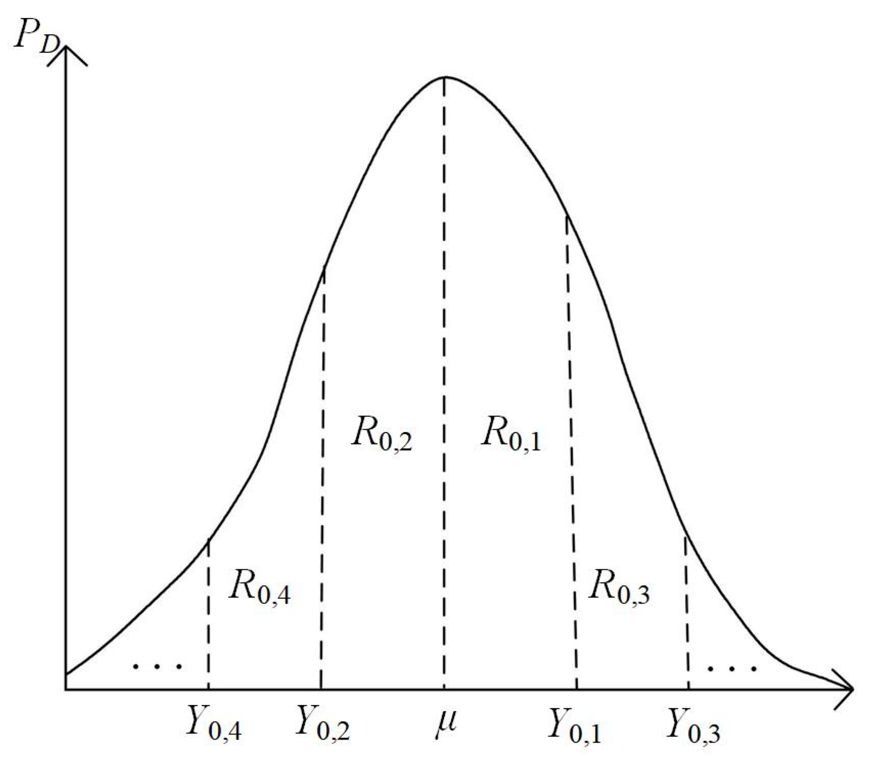
The multilinear Monte Carlo method is the linear processing of multiple uncertain variables. First, the probability distribution of the total load of the system is divided into m parts. Let every part be R0,i, which corresponds to Y0,i in the process of linear segmentation and correspondence (i = 1, 2, …, m), as shown in Figure 2. Then, after the probability distribution function of the total load is determined, the probability distribution function of wind power output power is also divided into m parts corresponding to the total load one by one.
Using the method of (33) to perform linear processing on each part gives
M 1 : Y t = Y 0 , 1 + J 1 1 [ X 1 μ ( X 1 ) ] M 2 : Y 2 = Y 0 , 2 + J 2 1 [ X 2 μ ( X 2 ) ] M m : Y m = Y 0 , m + J m 1 [ X m μ ( X 2 ) ]
The upper limit of the interval i is m, and Ji is the Jacobian matrix of Y0,i. The solution of the system power balance (18) is
g s ( Y 0 , j ) = μ ( X i )
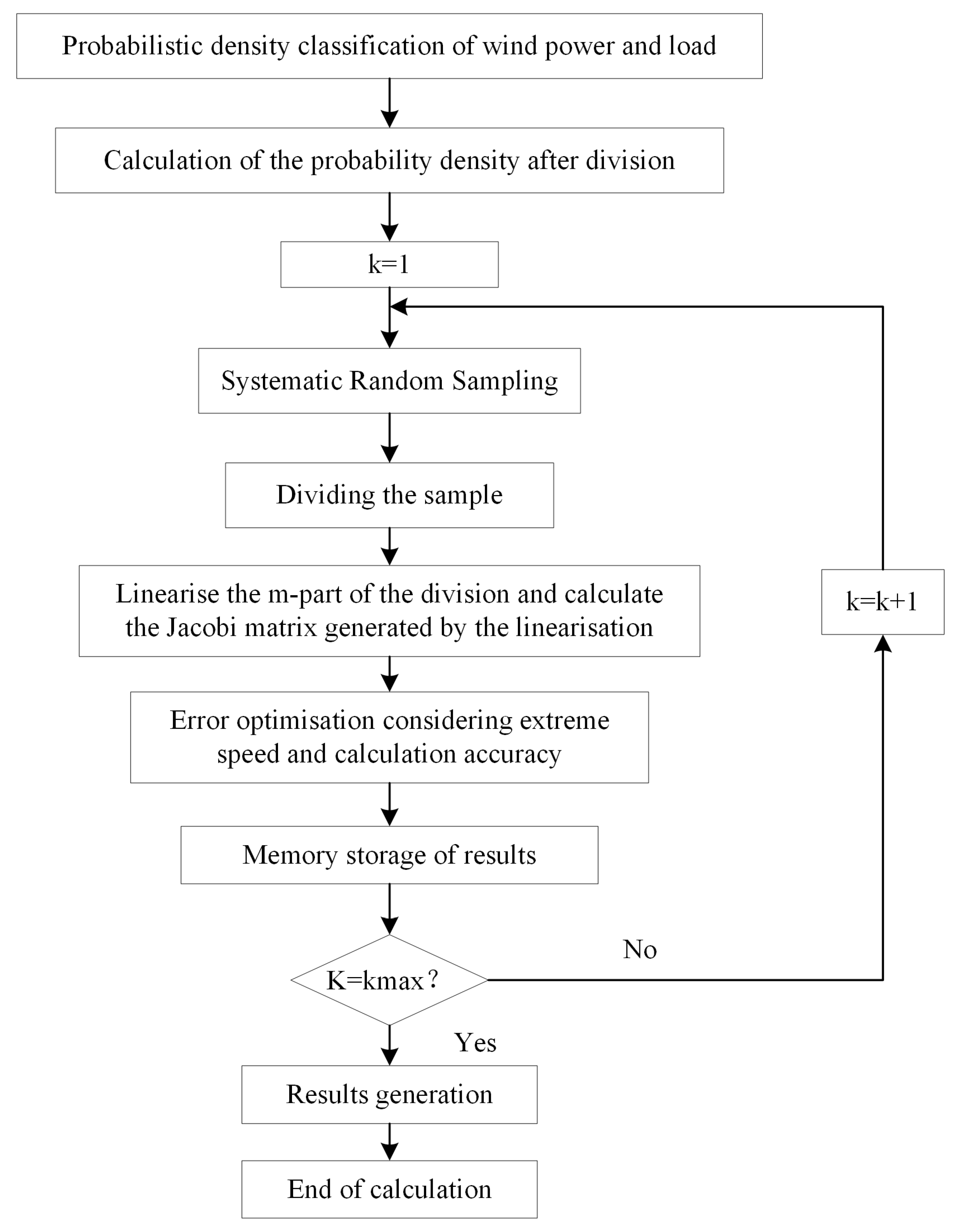
The calculation flow of the multilinear Monte Carlo method is shown in Figure 3, where k is the number of tests, and kmax is the upper limit of k. Using the multilinear Monte Carlo method, only part of the input of the optimization model can be obtained by sampling and calculating a planning scheme many times at a time. After that, we still need to use the optimization algorithm to solve the planning model to obtain the parameters of the system planning scheme. By solving this model, the optimal planning cost and renewable energy consumption parameters of the planning scheme can be converged.

4. Example Analysis

This chapter is the simulation section of an example. This part mainly verifies the validity of the multilinear Monte Carlo simulation algorithm through the uncertain behavior characteristics of the power supply side and the load side. The simulation results can provide a basis for decision making for a system planning scheme.

4.1. Simulation Model

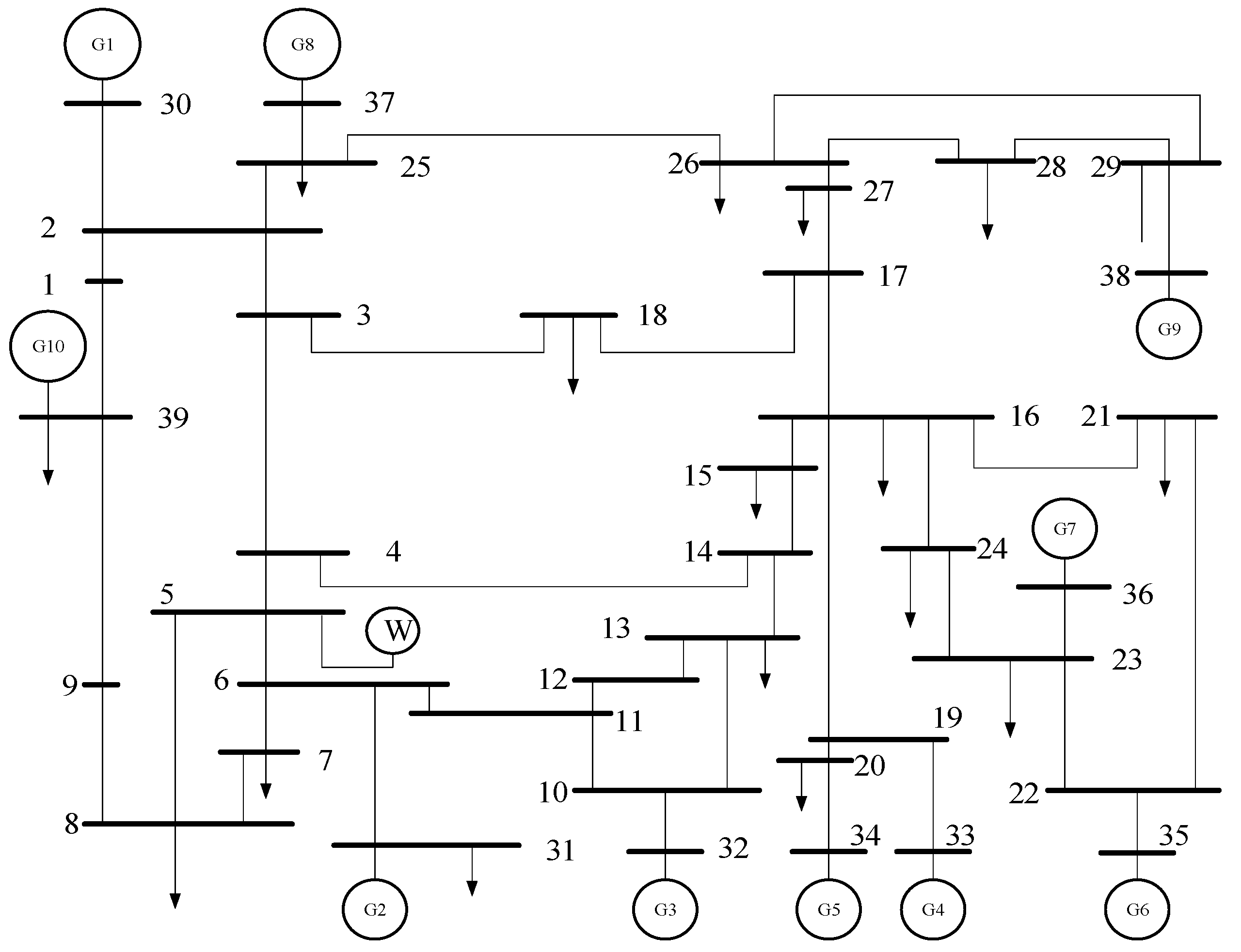
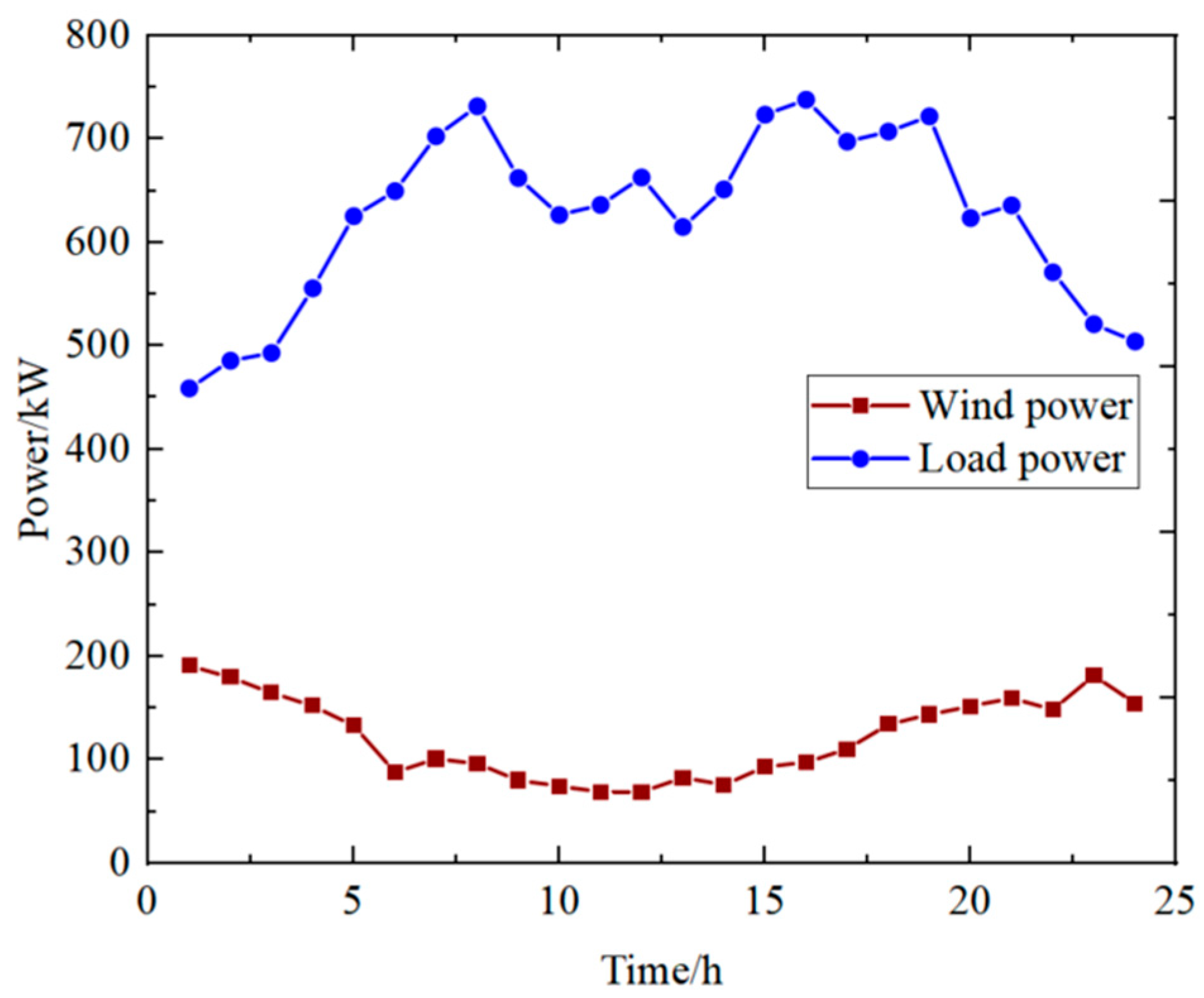
When the probability distribution of a load is known, the optimal programming model is solved by a sampling test based on the multilinear Monte Carlo method. In this paper, modified IEEE 39-bus test system data were used for the simulation, as shown in Figure 4. The data of thermal power units and wind turbines are shown in Table 1 and Table 2, respectively. Figure 5 shows the wind turbine output and load of a typical day.

4.2. Comparison of the Methods

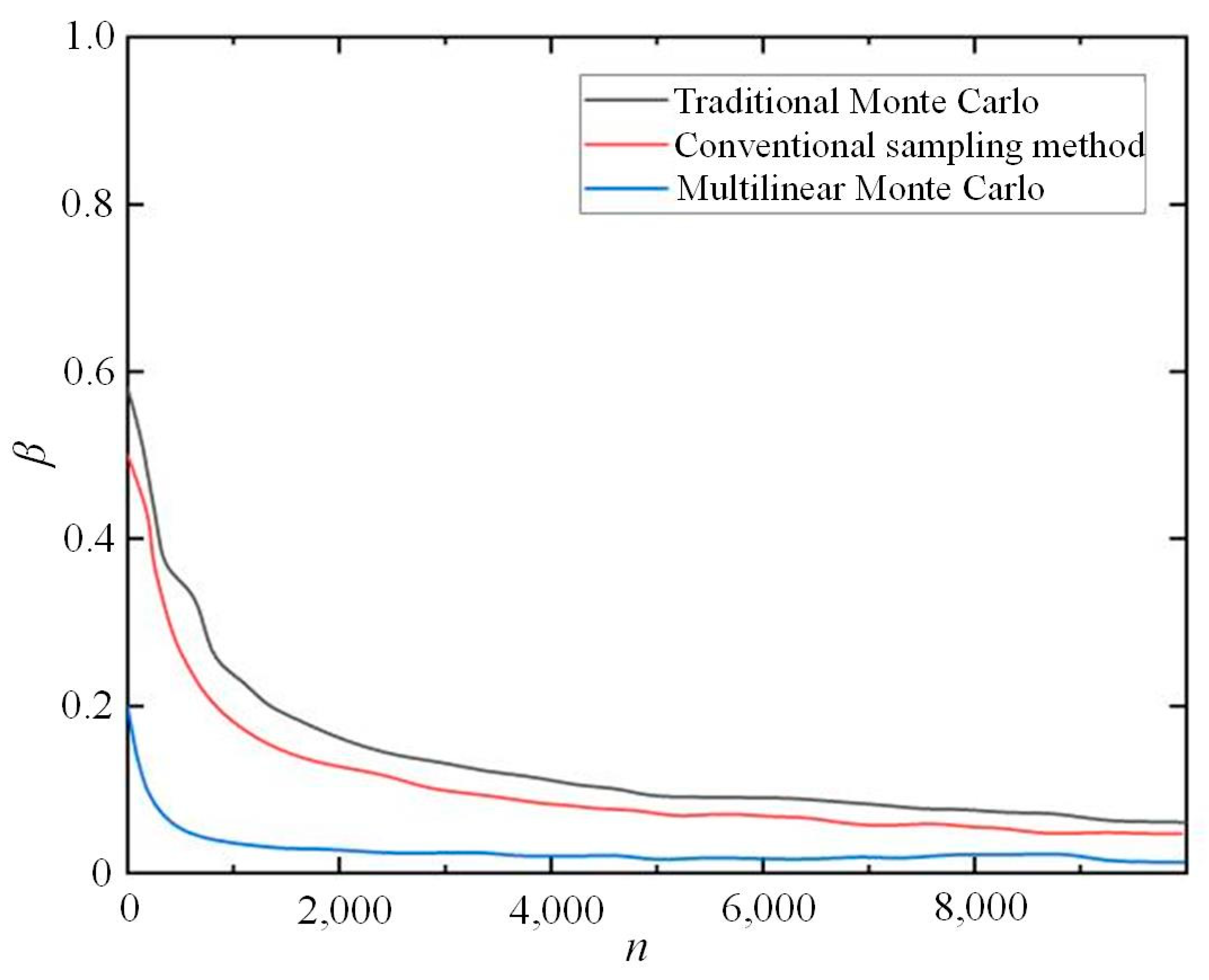
In this paper, the traditional Monte Carlo method, the traditional important sampling method, and the multilinear Monte Carlo method are compared and analyzed. Under the same sampling times, the sampling accuracy of the three methods is shown in Figure 6. It can be seen that the multilinear Monte Carlo method has the highest calculation precision in the whole sampling process. The corresponding curve changes smoothly. The other two corresponding curves fluctuate greatly. The results show that the multilinear Monte Carlo method is superior to the other methods.
The calculation efficiency of these three methods can be further verified. Table 3 shows the results of three different precision algorithms. Therefore, under different calculation accuracy requirements, the multilinear Monte Carlo method requires the lowest calculation time. Because the calculation of system control variables after each sampling does not involve power flow analysis and load shedding calculation, the amount of calculation for each system state analysis will not be increased. The multilinear Monte Carlo method is faster and more efficient under the same calculation accuracy.
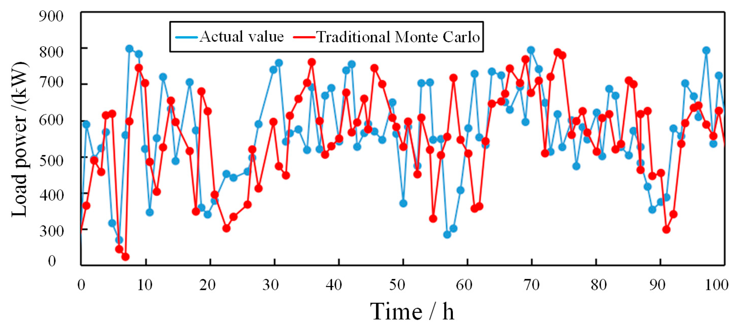
To verify the validity of the Monte Carlo method, the real value was compared with the actual value of load simulated by the two Monte Carlo methods, and the results are shown in Figure 7 and Figure 8 below. Obviously, for example, when t = 8, the actual value is 793 kW, the traditional Monte Carlo is 765 kW, and the multilinear Monte Carlo is 784 kW. When t = 21, the actual value is 385 kW, the traditional Monte Carlo is 313 kW, and the multilinear Monte Carlo is 355 kW. When t = 92, the actual value is 389 kW, the traditional Monte Carlo is 325 kW, and the multilinear Monte Carlo is 372 kW. The results show that, compared with the traditional Monte Carlo method, the calculation results of the multilinear Monte Carlo method are more in line with real values.
The calculation speed and accuracy of the multilinear Monte Carlo method were compared with the traditional Monte Carlo method as follows. Considering the combination of power load and power supply as known quantities, the existing data of the IEEE system are adopted here. The probability distribution of wind power output is a known quantity, while the power gap is an unknown quantity. Therefore, the user’s power supply gap in each time period will be calculated by the model, and this value can be determined as the real value. Then, through two Monte Carlo methods, through repeated sampling and simulation tests, the power supply shortage is obtained, which is defined as the calculated value of the two methods, and the difference between the calculated value and the real value is used as the calculation error. The advantages and disadvantages between the traditional Monte Carlo method and the multilinear Monte Carlo method were further analyzed by comparing the calculation error and calculation time.

4.3. Scheme Verification

After determining the best simulation method, according to the basic requirements of the IEEE system, the access points of wind power are G1 and G2, and there are three power planning schemes, regardless of all the power planning schemes of thermal power units, as shown in Table 4.
During the test, the maximum load of each node is extracted according to the normal distribution characteristics to determine the power capacity of different access points. According to known optional unit parameters, the simulation can be divided into four scenarios according to the load correlation and standard deviation ratio between the modified IEEE 39-bus test system, as shown in Table 5.
After the access point of the wind turbine is determined, each power unit has three planning schemes, and finally, these schemes are put into actual operation, which is calculated according to the running time of 1 week. The following Table 6 shows the simulation results under various scenarios.
According to the simulation results of the multilinear Monte Carlo method, the load correlation coefficient has little influence on the simulation results, but the standard deviation of the load has a great influence. When the standard deviation of the user load is small, the range of the load value is concentrated near the average, and the normal distribution image is higher at the average. At this time, the demand side of the system has high certainty, so the simulation results of the planning scheme are excellent. When the standard deviation of the load is large, the image of the normal distribution is flat, the load value is scattered, and the demand-side uncertainty to be dealt with in system planning is strong, so the simulation results are relatively poor.

5. Conclusions

In this paper, the coordinated planning of a power system under uncertain characteristics based on the multilinear Monte Carlo method was studied. Firstly, the characteristic model and probability density function of uncertain behavior on the power supply side and load sides of the system were established. Then, the coordinated planning scheme of the system was designed. According to the characteristics of multi-input and multioutput systems, the traditional Monte Carlo simulation method was improved as a multilinear Monte Carlo simulation method. This method was used to solve the coordination plan model. Finally, the modified IEEE 39-bus test system, as an example, was utilized to confirm the validity of this method. The results showed that the multilinear Monte Carlo method is beneficial for improving calculation accuracy by 2.39% and speed by 5.58%, promoting the controllability of the supply side and demand side of the system, and providing a reference for solving system planning problems aimed at reducing system operation costs and promoting the consumption of renewable energy.

Author Contributions

Methodology, L.Z.; Software, L.Z. and D.P.; Validation, Y.Z.; Formal analysis, Y.L.; Data curation, Y.L.; Visualization, D.P.; Supervision, Y.Z.; Project administration, Y.W.; Funding acquisition, Y.W. All authors have read and agreed to the published version of the manuscript.

Funding

This work was supported by the Science & Technology Project of State Grid Corporation of China (5100-202356418A-3-2-ZN).

Data Availability Statement

Data are contained within the article.

Conflicts of Interest

The authors declare that the research was conducted in the absence of any commercial or financial relationships that could be construed as a potential conflict of interest.

References

  1. Datta, J.; Das, D. Energy Management Study of Interconnected Microgrids Considering Pricing Strategy Under the Stochastic Impacts of Correlated Renewables. IEEE Syst. J. 2023, 17, 3771–3782. [Google Scholar] [CrossRef]
  2. Zhang, C.; Xu, Y.; Dong, Z.Y. Robustly Coordinated Operation of a Multi-Energy Micro-Grid in Grid-Connected and Islanded Modes Under Uncertainties. IEEE Trans. Sustain. Energy 2020, 11, 640–651. [Google Scholar] [CrossRef]
  3. Vu, D.H.; Muttaqi, K.M.; Sutanto, D. An Integrated Energy Management Approach for the Economic Operation of Industrial Microgrids Under Uncertainty of Renewable Energy. IEEE Trans. Ind. Appl. 2020, 56, 1062–1073. [Google Scholar]
  4. Ryu, J.; Kim, J. Virtual Power Plant Operation Strategy Under Uncertainty withs Demand Response Resources in Electricity Markets. IEEE Access 2022, 10, 62763–62771. [Google Scholar] [CrossRef]
  5. Fang, X.; Hodge, B.M.; Du, E.; Kang, C.; Li, F. Introducing Uncertainty Components in Locational Marginal Prices for Pricing Wind Power and Load Uncertainties. IEEE Trans. Power Syst. 2019, 34, 2013–2024. [Google Scholar] [CrossRef]
  6. Alanazi, M.S. A Modified Teaching—Learning-Based Optimization for Dynamic Economic Load Dispatch Considering Both Wind Power and Load Demand Uncertainties with Operational Constraints. IEEE Access 2021, 9, 101665–101680. [Google Scholar] [CrossRef]
  7. Neves, L.S.; Costa Alberto, L.F. On The Computation of The Locally Closest Bifurcation Point Considering Loading Uncertainties and Reactive Power Limits. IEEE Trans. Power Syst. 2020, 35, 3885–3894. [Google Scholar] [CrossRef]
  8. Wang, C.; Chu, S.; Ying, Y.; Wang, A.; Chen, R.; Xu, H.; Zhu, B. Underfrequency Load Shedding Scheme for Islanded Microgrids Considering Objective and Subjective Weight of Loads. IEEE Trans. Smart Grid 2023, 14, 899–913. [Google Scholar] [CrossRef]
  9. Liu, Y.; Su, T.; Qiu, G.; Gao, H.; Liu, J.; Shui, Y. Analytic Deep Learning and Stepwise Integrated Gradients-based Power System Transient Stability Preventive Control. IEEE Trans. Power Syst. 2023, 10, 1–14. [Google Scholar] [CrossRef]
  10. Liu, Y.; Gao, S.; Qiu, G.; Liu, T.; Ding, L.; Liu, J. A Physics-Informed Action Network for Transient Stability Preventive Control. IEEE Trans. Power Syst. 2023, 38, 1771–1774. [Google Scholar] [CrossRef]
  11. Mathias, J.; Bušić, A.; Meyn, S. Load-Level Control Design for Demand Dispatch with Heterogeneous Flexible Loads. IEEE Trans. Control Syst. Technol. 2023, 31, 1830–1843. [Google Scholar] [CrossRef]
  12. Qiu, G.; Liu, Y.; Liu, J.; Wang, L.; Liu, T.; Gao, H.; Jawad, S. Surrogate-Assisted Optimal Re-Dispatch Control for Risk-Aware Regulation of Dynamic Total Transfer Capability. IET Gener. Transm. Distrib. 2021, 15, 1949–1961. [Google Scholar] [CrossRef]
  13. Qiu, G.; Liu, Y.b. Analytic Deep Learning-Based Surrogate Model for Operational Planning with Dynamic TTC Constraints. IEEE Trans. Power Syst. 2020, 36, 3507–3519. [Google Scholar] [CrossRef]
  14. Gao, Q.; Liu, Y.; Zhao, J.; Liu, J.; Chung, C.Y. Hybrid Deep Learning for Dynamic Total Transfer Capability Control. IEEE Trans. Power Syst. 2021, 36, 2733–2736. [Google Scholar] [CrossRef]
  15. Liu, X.; Liu, Y.; Liu, J.; Xiang, Y.; Yuan, X. Optimal Planning of AC-DC Hybrid Transmission and Distributed Energy Resource System: Review and Prospects. CSEE J. Power Energy Syst. 2019, 5, 409–422. [Google Scholar] [CrossRef]
  16. Fan, H.; Yu, Z.; Xia, S.; Li, X. Review on Coordinated Planning of Source-Network-Load-Storage for Integrated Energy Systems. Front. Energy Res. 2021, 9, 641158. [Google Scholar] [CrossRef]
  17. Du, E.; Zhang, N.; Kang, C.; Xia, Q. A High-Efficiency Network-Constrained Clustered Unit Commitment Model for Power System Planning Studies. IEEE Trans. Power Syst. 2019, 34, 2498–2508. [Google Scholar] [CrossRef]
  18. Huang, W.; Zhang, X.; Li, K.; Zhang, N.; Strbac, G.; Kang, C. Resilience Oriented Planning of Urban Multi-Energy Systems with Generalized Energy Storage Sources. IEEE Trans. Power Syst. 2022, 37, 2906–2918. [Google Scholar] [CrossRef]
  19. Ahmad, T.; Zhang, D. Novel Deep Regression and Stump Tree-Based Ensemble Models for Real-Time Load Demand Planning and Management. IEEE Access 2020, 8, 48030–48048. [Google Scholar] [CrossRef]
  20. Suo, X.; Zhao, S.; Ma, Y.; Dong, L. New Energy Wide Area Complementary Planning Method for Multi-Energy Power System. IEEE Access 2021, 9, 157295–157305. [Google Scholar] [CrossRef]
  21. Bolgaryn, R.; Wang, Z.; Scheidler, A.; Braun, M. Active Power Curtailment in Power System Planning. IEEE Open Access J. Power Energy 2021, 8, 399–408. [Google Scholar] [CrossRef]
  22. Wu, X.; Jiang, Y. Source-Network-Storage Joint Planning Considering Energy Storage Systems and Wind Power Integration. IEEE Access 2019, 7, 137330–137343. [Google Scholar] [CrossRef]
  23. Li, P.; Song, Y.D.; Li, D.Y.; Cai, W.C.; Zhang, K. Control and Monitoring for Grid-Friendly Wind Turbines: Research Overview and Suggested Approach. IEEE Trans. Power Electron. 2015, 30, 1979–1986. [Google Scholar] [CrossRef]
  24. Avramidis, I.; Capitanescu, F.; Deconinck, G. Grid-Friendly Smart Sustainable Buildings: Flexibility-to-Cost Mapping. IEEE Trans. Sustain. Energy 2022, 13, 1857–1860. [Google Scholar] [CrossRef]
  25. Afrasiabi, M.; Mohammadi, M.; Rastegar, M.; Stankovic, L.; Afrasiabi, S.; Khazaei, M. Deep-Based Conditional Probability Density Function Forecasting of Residential Loads. IEEE Trans. Smart Grid 2020, 11, 3646–3657. [Google Scholar] [CrossRef]
  26. Bich, W. From Errors to Probability Density Functions. Evolution of the Concept of Measurement Uncertainty. IEEE Trans. Instrum. Meas. 2012, 61, 2153–2159. [Google Scholar] [CrossRef]
  27. Eggermont, P.B.; LaRiccia, V.N. Best Asymptotic Normality of the Kernel Density Entropy Estimator for Smooth Densities. IEEE Trans. Inf. Theory 1999, 45, 1321–1326. [Google Scholar] [CrossRef]
  28. Zhu, X.; Di Rienzo, L.; Ma, X.; Codecasa, L. Multilevel Monte Carlo FDTD Method for Uncertainty Quantification. IEEE Antennas Wirel. Propag. Lett. 2022, 21, 2030–2034. [Google Scholar] [CrossRef]
  29. Du, H.; Xie, W.; Liu, Z.; Li, L. Track-Oriented Marginal Poisson Multi-Bernoulli Mixture Filter for Extended Target Tracking. Chin. J. Electron. 2023, 32, 1106–1119. [Google Scholar] [CrossRef]
  30. Qi, C.; Yin, J.; Niu, Y.; Xu, J. Neighborhood Spatial Aggregation MC Dropout for Efficient Uncertainty-Aware Semantic Segmentation in Point Clouds. IEEE Trans. Geosci. Remote Sens. 2023, 61, 1–16. [Google Scholar] [CrossRef]
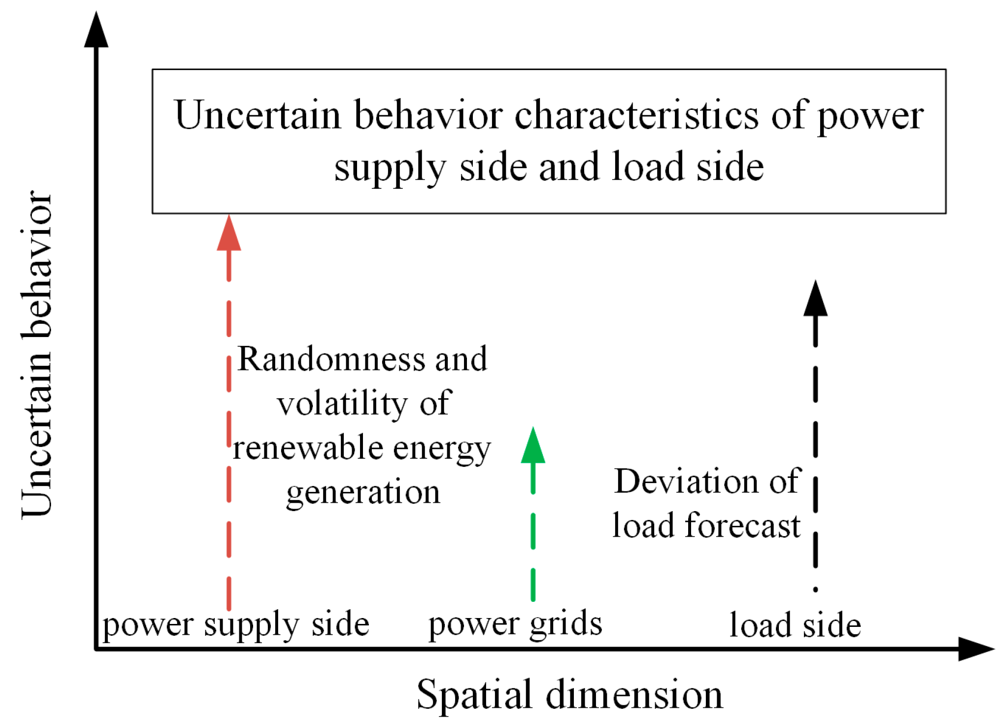
Figure 1. Schematic diagram of system uncertainty behavior characteristics.
Energies 16 07761 g001
Figure 2. Separation of the probability density function.
Energies 16 07761 g002
Figure 3. Calculation flow chart of multilinear Monte Carlo method.
Energies 16 07761 g003
Figure 4. Topology diagram of modified IEEE 39-bus test system.
Energies 16 07761 g004
Figure 5. Wind turbine output and load of a typical day.
Energies 16 07761 g005
Figure 6. Comparison chart of sampling accuracy of different methods.
Energies 16 07761 g006
Figure 7. Comparison results between the traditional Monte Carlo method and real value.
Energies 16 07761 g007
Figure 8. Comparison results between the multilinear Monte Carlo method and real value.
Energies 16 07761 g008
Table 1. Data of thermal power units.
Unit ModelCost of Investment
(Ten Thousand Yuan/MW)
Maximum Output
(MW)
Minimum Output
(MW)
11505030
22006035
32207030
42508035
Table 2. Wind turbine data.
Rated Wind Speed
(m/s)
Cut-In Wind Velocity
(m/s)
Cut Wind Speed
(m/s)
Cost of Investment
(Ten Thousand Yuan/kW)
123.3200.3
Table 3. Calculation results of three methods with different accuracy.
βMethodSampling TimeTime/s
0.08Traditional Monte Carlo801398.28
Conventional sampling method497572.40
Multilinear Monte Carlo29617.42
0.1Traditional Monte Carlo481660.43
Conventional sampling method357048.25
Multilinear Monte Carlo20414.54
0.15Traditional Monte Carlo234742.37
Conventional sampling method157634.51
Multilinear Monte Carlo12812.14
Table 4. Power access scheme.
CaseG1G2Other Node
a××
b××
c×
The sign “√” indicates that the node has a power supply. The symbol “×” indicates that the node has no power supply.
Table 5. Values of four scenario parameters.
ScenarioLoad Correlation FactorStandard Deviation
10.50.2 μ
20.50.3 μ
30.90.2 μ
40.90.3 μ
Table 6. Simulation results of different scenarios.
ScenarioCaseRunning Cost
(Ten Thousand Yuan)
Daily Wind Power Consumption (MW·h)Economic Growth RateRenewable Energy Consumption Growth Rate
1a36,713.3663,90815%2.04%
b37,423.7165,42016%2.13%
c56,611.53125,02425%3.81%
2a41,363.3158,70313%1.85%
b45,853.1156,96315%1.91%
c67,346.21109,63520%2.98%
3a38,743.2566,43716%2.11%
b37,835.9765,37118%2.28%
c58,637.54119,63527%3.84%
4a43,306.2358,70314%1.74%
b47,261.3452,96317%1.87%
c67,791.47108,63521%2.78%
Disclaimer/Publisher’s Note: The statements, opinions and data contained in all publications are solely those of the individual author(s) and contributor(s) and not of MDPI and/or the editor(s). MDPI and/or the editor(s) disclaim responsibility for any injury to people or property resulting from any ideas, methods, instructions or products referred to in the content.