Article

Analysis of Uneven Distribution of Nodes Creating a Percolation Channel in Matrices with Translational Symmetry for Direct Current

1
Department of Economics, Vincent Pol University in Lublin, 2, Choiny Str., 20-816 Lublin, Poland
2
Department of Electrical Devices and High Voltage Technology, Faculty of Electrical Engineering and Computer Science, Lublin University of Technology, 38A, Nadbystrzycka Str., 20-618 Lublin, Poland
*
Author to whom correspondence should be addressed.
Energies 2023, 16(22), 7647; https://doi.org/10.3390/en16227647
Submission received: 28 October 2023 / Revised: 13 November 2023 / Accepted: 15 November 2023 / Published: 18 November 2023

Abstract

:
In this study, the phenomenon of node percolation was tested using the Monte Carlo computer simulation method for square matrices with dimensions L = 55, 101 and 151. The number of samples for each matrix was 5 × 10⁶. The spatial distributions of the coordinates of the nodes creating the percolation channel were determined, and maps of the density distribution of these nodes were created. It has been established that in matrices with finite dimensions, an edge phenomenon occurs, consisting of a decrease in the concentration of nodes creating a percolation channel as one approaches the edge of the matrix. As the matrix dimensions increase, the intensity of this phenomenon decreases. This expands the area in which values close to the maximum occur. The length distributions of the left and right clusters of non-conducting nodes were determined for the situation when the next randomly selected node connects them and thus reaches the percolation threshold. It was found that clusters whose dimensions are close to half of the matrix dimensions are most likely to occur. The research shows that both the values of the standard deviation of the percolation threshold and the intensity of the edge phenomenon are clearly related to the dimensions of the matrices and decrease as they increase.

1. Introduction

The study of the phenomenon known as percolation, derived from the Latin ‘percolatio’, is primarily aimed at studying the permeation of liquids and gases through porous substrates [1]. Percolation issues have ubiquitous applications in a variety of scientific and technological research fields, including chemistry [2], medicine [3], biology [4] and materials engineering [5]. In addition, the conceptual framework of percolation extends its utility to the determination of the propagation of electric current in entities characterized by disordered semiconductors [6].
The study of the percolation phenomenon is directed in two basic directions. One of these involves empirical research, during which the simplest way to observe a phenomenon is via the conduit of electric current [7]. Conversely, endeavors directed at the examination of gas or liquid flow have proved considerably more intricate to execute.
To observe the classical phenomenon of percolation in the context of electric current flow, certain preconditions must be met. The medium in which percolation occurs should consist of at least two phases. The first is referred to as the matrix, while the elements forming the second phase, referred to as the dispersed phase, are distributed throughout the matrix. The properties of these phases should differ significantly. Typically, the matrix is an insulating material, and the dispersed phase is conductive elements with macroscopic dimensions. As the concentration of the dispersed phase in the composite increases, its components form electrical connections via points of contact, gradually forming a complex network of structures known as clusters. When a certain critical concentration, known as the percolation threshold, is reached, a so-called infinite cluster connecting the electrodes, known as a percolation channel, is formed. There is a rapid change in the macroscopic electrical properties of the medium. In the case of metal–dielectric composites or nanocomposites, there is a sharp drop in resistivity and a change in the type of conductivity from dielectric to metallic [8]. Dielectric conductivity is characterized by the fact that the resistivity of the medium decreases with increasing temperature. However, in the case of metallic conductivity, resistivity increases with increasing temperature [9]. This is a type 2 phase transition.
As is known, the conventional limit between composites and nanocomposites is approximately 100 nm [10]. When at least one of the dimensions of the dispersed phase elements is below this limit, we are dealing with nanocomposites. Based on experimental studies, it was determined that the value of the percolation threshold in metal–dielectric nanocomposites depends on the material of the dispersed phase placed in matrices of various compositions. The percolation threshold can vary over a very wide range, starting from a few percent [11,12,13,14] to values close to 50% [15,16].
The phenomenon of percolation has been used in the description of various issues, such as the spread of epidemics [17,18,19], the reliability of computer networks [20] and the spread of fires [21,22], as well as in molecular biology [23], materials engineering [24,25] or the flow of electric current through conductive and non-conductive mixtures [26,27]. In recent decades, the percolation phenomenon has been successfully used to describe current conduction in metal–dielectric nanocomposites [28,29,30]. This is hopping conductivity based on the quantum mechanical phenomenon of electron tunneling [31,32,33,34]. Without taking this phenomenon into account, it is impossible to understand and explain the dependence of the current intensity in nanocomposites on the metallic phase content, current frequency and temperature.
The second line of research is theoretical research and modeling [35,36,37]. For a longer period, studies involving the simulation of percolation in two-dimensional networks with translational symmetry were mainly used to illustrate this phenomenon. Subsequent work in this direction amounted to more and more precise determination of the percolation threshold value [38,39,40,41]. Yes, it is interesting from the point of view of numerical calculations. However, such high accuracy is not needed, for example, in the analysis of experimental results.
In recent decades, a new field of materials has emerged, so-called 2D materials. These are two-dimensional materials with a thickness of one to several atoms. Such materials include graphene, MXenes and a number of others [42,43,44,45,46,47,48,49,50,51,52,53,54,55].
The structure of two-dimensional composites may contain atoms of impurities, as well as vacancies and internodes. This is evidenced, for example, by the observation of step conductivity caused by electron tunnelling in MXene-PCL nanocomposites [56]. As is known, tunnelling occurs when there are closely located potential wells with nanometer dimensions in the material [57]. This means that potential wells exist in MXene-PCL nanocomposites, created by inclusions with dimensions of one or several atoms. Positron annihilation studies [58] have shown that inclusions can be, for example, divacancy + an oxygen atom in the internode or vacancy + two oxygen atoms located in the internode.
The analysis of the distribution of such inclusions in 2D materials exactly coincides with the analysis of the percolation phenomenon in two-dimensional matrices with translational symmetry. Therefore, research on percolation in 2D lattice systems with translational symmetry, which was initially only model or illustrative, together with the development of technology for producing 2D materials, may discover both scientific, applied and practical features.
In this work, the percolation of nodes in square matrices was selected for analysis. This choice is because such matrices have high symmetry and are the least complicated systems compared to triangular, honeycomb and other even more complex matrices. The choice of the simplest and most symmetrical shape is since the properties of the percolation process in the case of complex networks may be masked by the geometric and analytical intricacies of complicated network models
Therefore, the aim of the work was:
  • determining the value of the percolation threshold and the coordinates of the node interrupting the last percolation channel for each trial;
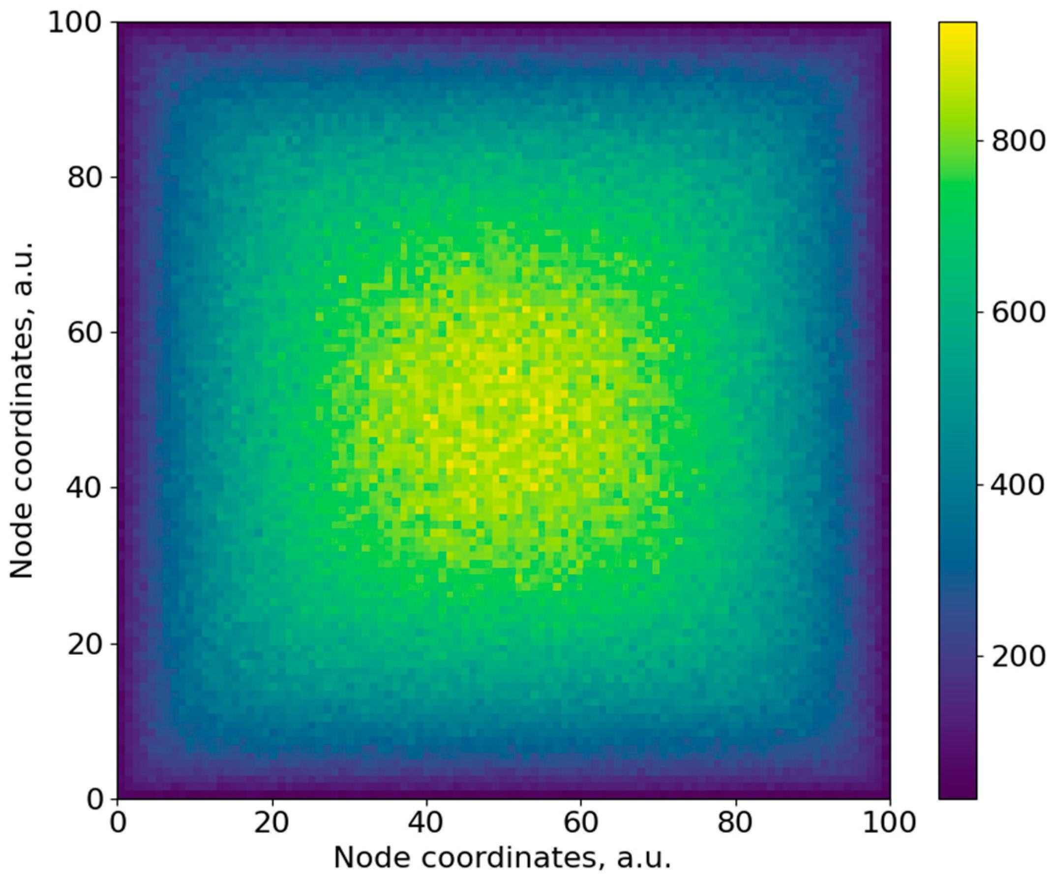
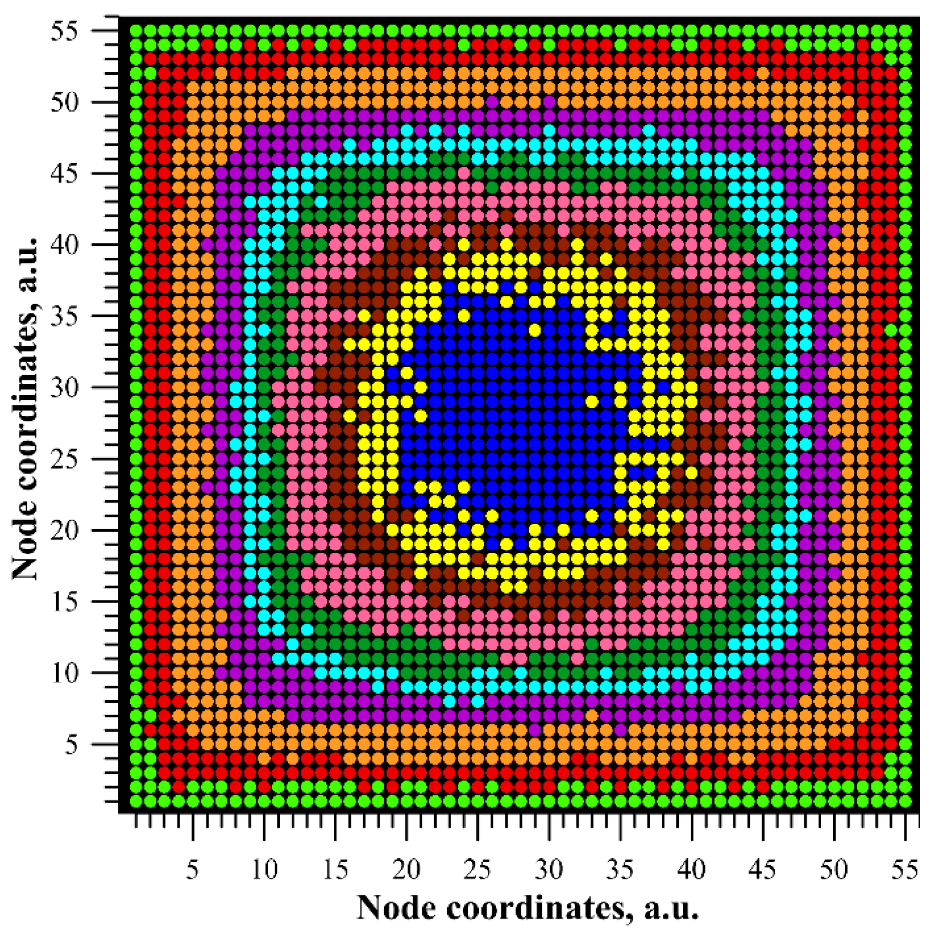
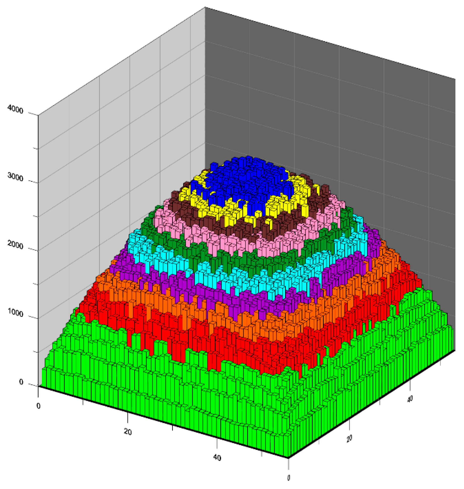
  • development of maps and spatial distributions of nodes creating the percolation channel and the standard deviation of the percolation threshold;
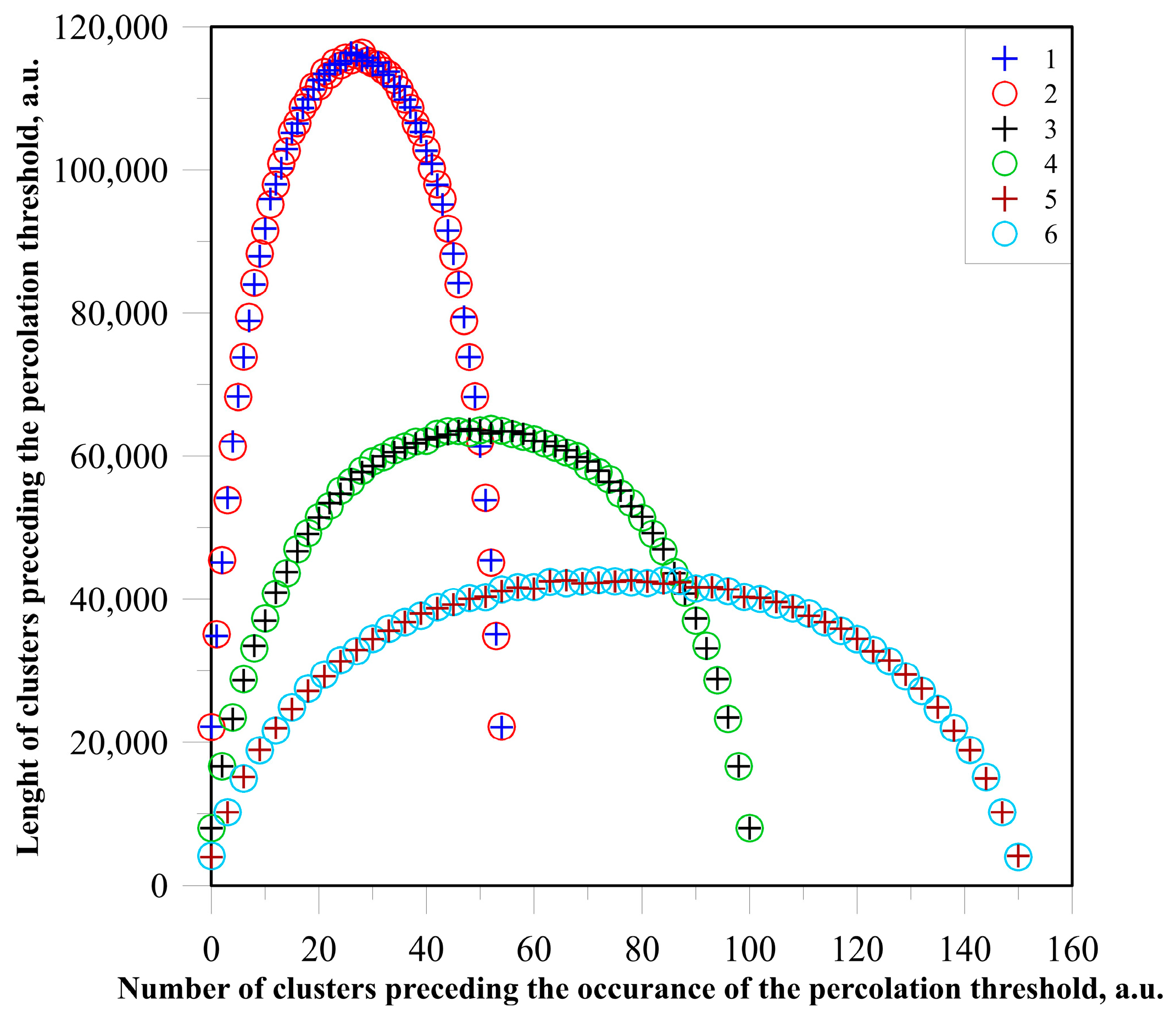
  • analysis of the probability of occurrence of clusters depending on their dimensions.

2. Research Method

The programming language Python was used to create the algorithm and simulation program for this study, with a detailed explanation provided in [59]. This work verified the correct operation of the program. Set theory served as the foundation for the calculations, as computers execute assignment processes significantly more quickly than computational processes. The dimension of the square network L was the sole variable. The ‘Mersenne Twister’ algorithm [60] used, a pseudo-random number generator, is often used in Monte Carlo simulations, as mentioned in [61,62]. A sequential selection of non-conducting nodes was carried out by the program. The initial node, randomly selected, constituted a set of a single element. Each subsequently chosen non-conducting node was then assessed to determine if it was part of any existing sets, that is, whether the selected node was within a one-unit distance vertically, horizontally or diagonally from any node in the preexisting set. Adding it to this set resulted in the formation of a cluster. In other cases, the node constituted a single-element set. An exception occurred when the selected node belonged to multiple clusters, when it was added to the merged clusters. Following the addition of a non-conducting node to an existing cluster, this cluster underwent a test to verify whether it contained points with coordinates x = 1 and x = L. This condition ascertained whether the cluster established a continuous connection between the right and left edges of the matrix. Meeting these criteria results in the formation of what is known as the ‘infinite cluster’ of non-conducting nodes and the attainment of the percolation threshold. During this step, the algorithm documented the coordinates of the initial randomly chosen node, the coordinates of the non-conducting node that disrupted the most recent percolation channel and the computed percolation threshold concentration and subsequently completed its operation. The algorithm was executed repeatedly until the specified number of samples, which was 5 million, was achieved. Simulations were conducted for matrices of sizes L = 55, 101 and 151.

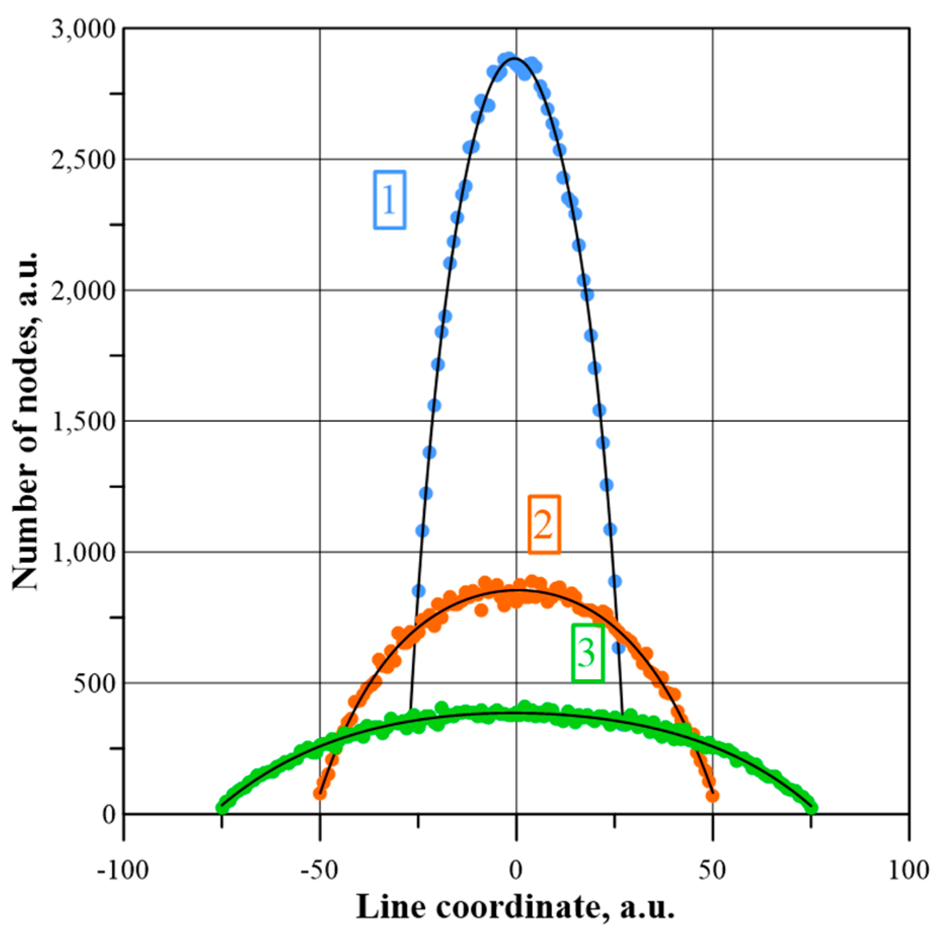
3. Edge Phenomenon of Spatial Distribution of Nodes Forming a Percolation Channel

It was established that the percolation threshold values for matrices with dimensions L = 51, 101, 151 and sample numbers 5 × 10⁴ and above do not depend on the matrix dimensions. In contrast, the values of the standard deviations decrease markedly with increasing matrix dimensions. In order to determine the sources of this phenomenon, maps of the spatial distribution of the nodes forming the percolation channel were made for matrices of dimensions 55, 101 and 151 for a sample number of 5 × 10⁶. For this purpose, the coordinates of the non-conducting node that interrupts the last percolation channel were determined via Monte Carlo simulations in each sample. Figure 1 shows, as an example, a heat map [63] of the two-dimensional distribution of the nodes that form the percolation channel for a matrix of dimension 101.
Figure 1 shows that there is an edge phenomenon in the matrices, which is that the nodes that form the percolation threshold are concentrated in the central part of the matrix. As each edge is approached, the number of these nodes decreases. In the central part, the number of nodes forming the percolation threshold is about an order of magnitude higher than the one near the edge.
In order to determine the sources of the decrease in the standard deviations of the percolation thresholds as the dimensions of the matrices increased, maps of the spatial distributions of the concentrations of the non-conducting nodes forming the percolation channel were made. Maps were made for matrices of dimensions 55, 101 and 151. To create the maps in a spreadsheet, after 5 × 10⁶ samples had been performed, the coordinates of all matrix nodes were recorded along with the assigned numbers of non-conducting nodes forming the percolation channel. An ascending sorting of the results was then performed according to the number of nodes forming the percolation channel located in the matrix nodes. After this, ranges of numbers of non-percolating nodes were selected to divide the matrix into 10 zones. Table 1 shows the ranges of change in the number of nodes forming the percolation threshold in each zone and the colours of the nodes in the spatial maps, corresponding to each zone.
Figure 2 shows, as an example, the two-dimensional distribution of non-conductive nodes forming the percolation channel per node for a matrix with L = 55 divided into 10 zones.
Figure 2 perfectly illustrates the edge phenomenon, whereby the concentration of nodes forming the percolation channel decreases as the edge of the matrix is approached. Analysis of the spatial maps (Figure 2) has shown that, firstly, the distribution of nodes forming the percolation channel in the zones, closest to the centre of the matrix, is close to circular. Secondly, for nodes in further zones, there is a fourth-order axis of symmetry passing through the centre of the matrix perpendicular to it. This is characteristic of square matrices with L × L dimensions. Thirdly, the closer to the edge, the closer the zone shape is to square. Fourthly (Table 1), the highest density of nodes forming the percolation channel is near the centre of the matrix. The further away from the centre, the lower the content of these nodes. It is also evident from Figure 2 that a small proportion of the nodes, belonging to one zone, are located between the nodes of neighbouring zones. The shuffling of some of the nodes near the zone boundary is related to the fact that the boundary between zones is unitary and the distribution of percolation threshold values is a random distribution. For example, for a matrix with L = 55, the upper boundary of zone 2 is 999, while the lower boundary of zone 3 is 1000.
In order to describe the edge phenomenon numerically, Figure 3 shows the spatial distributions of the coordinates of the nodes forming the percolation channel. The distributions were determined along lines passing through the centres of the matrices perpendicular to the edges. The continuous lines in Figure 3 show the polynomial approximations of order six of the simulation results. The values of the coefficients of determination R2 for the approximation waveforms are close to unity and are 0.9986, 0.9910 and 0.9863 for matrices of dimensions L = 55, 101 and 151, respectively. The closeness to unity of the R2 coefficients indicates a good-quality approximation. Figure 3 shows that the highest concentration of nodes forming the percolation channel occurs near the centre of the matrix. As one moves away from the centre, the concentration of these nodes decreases. It is also evident from the figure that as the matrix dimensions increase, there is a slowdown in the rate of decrease in the concentration of nodes, forming the percolation threshold, towards the edges.
The intensity of this phenomenon decreases with increasing matrix dimensions. The edge phenomenon observed in this work for percolation in finite-dimensional matrices is very similar, from a qualitative point of view, to the laminar flow of a liquid through a pipe. There too, the highest flow velocity occurs at the centre of the pipe and the lowest at the inner surface [64].

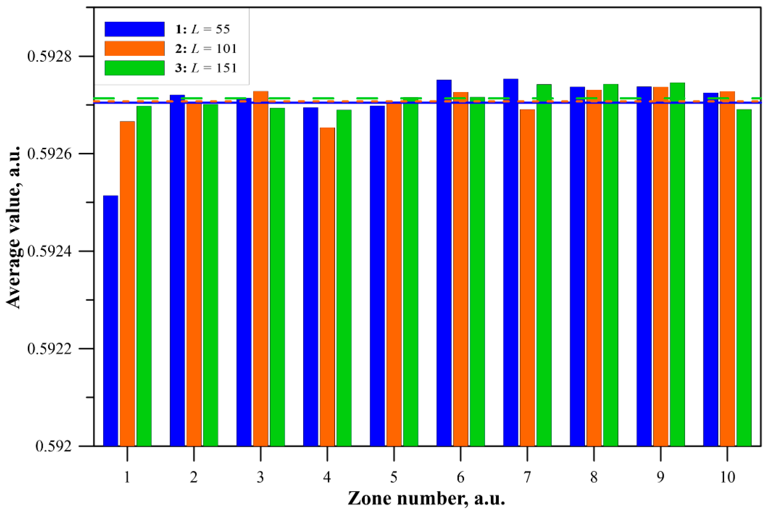
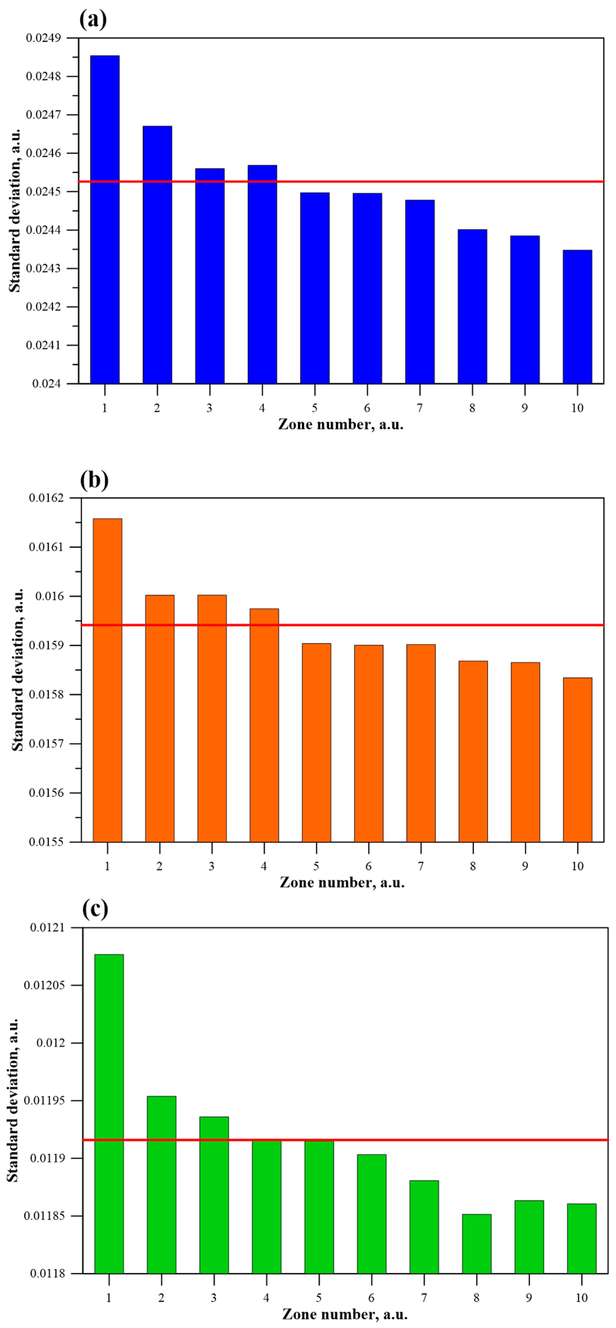
4. Spatial Distributions of Standard Deviation

The figures shown in Table 1 are not useful for comparing standard deviation values. This is because each zone has a different number of nodes forming the percolation channel. Therefore, it proved impossible to compare the standard deviation values of the percolation threshold for different zones.
In order to compare the values of the standard deviations in the different zones, the matrix was divided into 10 zones, each containing an equal number of nodes forming the percolation channel of 5 × 10⁵. To obtain this division, the coordinates of all the nodes of the matrix were recorded in a spreadsheet, together with the numbers of non-conductive nodes forming the percolation channel assigned to them. An ascending sorting of the results was then performed according to the number of non-conductive nodes forming the percolation channel located in the matrix nodes. A summation of the number of non-conductive nodes with the ascending result was then performed. In the zone numbered 1 ≤ i ≤ 10, there are coordinates of nodes for which the sum of the number of nodes forming the percolation channel Σ(i) is in the range
[ ( i 1 ) 5 10 5 + 1 ] ( i ) i 5 10 5
In this way, 10 zones were created, each containing 5 × 10⁵ nodes, forming a percolation channel. Using a spreadsheet, three-dimensional spatial distributions of the nodes forming the percolation channel were plotted. Figure 4 shows, as an example, the three-dimensional spatial distribution of the nodes, forming the percolation channel for a matrix of size L = 55 for a sample number of 5 × 10⁶. In the XY plane, the coordinates of the nodes of the square network are given. On the other hand, the values of the numbers of nodes forming the percolation channel per nodes of the square network were deposited along the vertical Z axis.
Figure 2, Figure 3 and Figure 4 show that the highest concentration of nodes forming the percolation channel is found in the central part of the matrix. As one approaches the edge of the matrix, the concentration of nodes forming the percolation channe repeatedly decreases.
Based on the division into ten zones containing 5 × 10⁵ nodes forming the percolation channel each, the mean values of the percolation thresholds and standard deviations were calculated, as shown in Table 2.
Figure 5 shows a histogram of the average values of the percolation threshold for the individual zones for matrices of 55, 101 and 151. The horizontal lines show the average values for the matrices. It can be seen from the figure that the lowest percolation threshold value occurs for zone 1 (outer) for a matrix with L = 55. The difference between the average value for the whole matrix and zone 1 is, however, very small, at around 0.00018. In this zone, as the matrix dimensions increase, the percolation threshold value approaches the average value for the whole matrix. In the following zones, random fluctuations in the percolation threshold value are observed. The difference between the smallest and largest results for zones 2 to 10 is less than 0.0001. This means that only for the matrix with L = 55 does the edge phenomenon have a slight effect on the percolation threshold value.
Figure 6 shows histograms of the standard deviation values for 10 zones containing 5 × 10⁵ samples each and the average values for matrices of dimensions 55, 101 and 151. It can be seen from the figure that the edge phenomenon manifests itself in that the standard deviation values increase as the edge of the matrix is approached. The rate of change of the standard deviation in the zones decreases with increasing die dimensions. The differences in standard deviations between zone 1 and zone 10 are approximately 0.0005 for a die with L = 51, 0.00032 for L = 101 and 0.00021 for L = 151. Based on the analysis of the results for matrices with L = 51, 101 and 151, it can be concluded that increasing the die dimensions reduces the effect of the edge phenomenon on the spatial distributions of the standard deviation values.

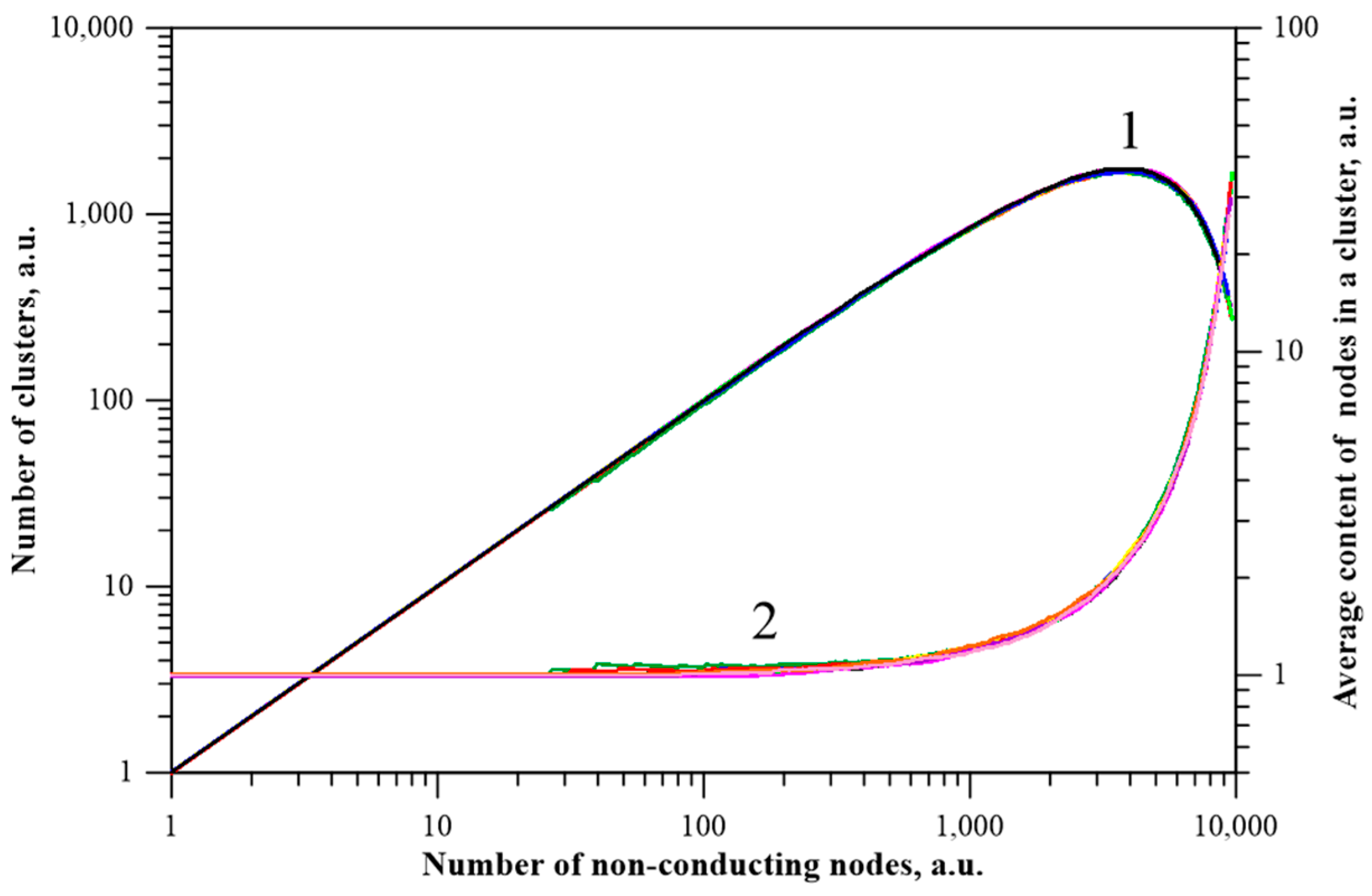
5. Analysis of the Size and Number of Non-Conductive Clusters as a Function of Matrix Dimensions

To further clarify the nature of the edge phenomenon, Figure 7, as an example, shows the dependence of the number of clusters consisting of non-conductive nodes on the number of non-conductive nodes inserted into a matrix with L = 151. The figure also shows the average number of non-conductive nodes in the clusters.
Figure 7 shows, as an example, the waveforms for 10 randomly selected samples. As can be seen from the figure, initially the clusters consist of single non-conductive nodes. As the number of introduced non-conductive nodes increases, a deviation from a linear relationship begins to occur, caused by an increase in the number of non-conductive nodes in the clusters. This is achieved by attaching the newly drawn non-conductive nodes to the existing ones. When a certain number of introduced non-conductive nodes is reached, the number of clusters reaches a maximum value. For a matrix with L = 55, this number is about 6 × 10², for L = 101—about 1.8 × 10³ and for L = 151—about 4 × 10³. With a further increase in the number of non-conductive nodes, the number of clusters starts to decrease. At the same time, the average number of non-conductive nodes per cluster increases rapidly. This is because newly introduced nodes connect neighbouring clusters to each other. The percolation threshold is reached when two adjacent clusters, one starting at the left edge of the matrix and the other starting at the right edge, are joined together. The sum of the lengths of these two clusters along the horizontal axis is L−1. Placing another non-conducting node between them results in a so-called infinite cluster, extending from one side edge of the matrix to the other. An infinite cluster composed of non-conductive nodes interrupts the possibility of current flow between the top and bottom edges of the matrix. The waveforms in Figure 7 end when the infinite cluster is formed and the percolation threshold is thus reached. It should be noted that a number of smaller clusters remain in the matrices after the percolation threshold is reached. Thus, in a matrix with L = 55, about 50 clusters remain, with an average number of non-conductive nodes in each cluster of about 25. In a matrix with L = 101, about 200 clusters remain, with an average number of nodes of about 25. In contrast, in a matrix with L = 151, the numbers are about 300 and about 30, respectively.
Figure 8 shows the length distributions of the left and right clusters preceding the percolation threshold for matrices with L = 55, 101 and 151 for a sample number of 5 × 10⁶. Drawing the next non-conductive node breaks the last percolation channel. Cluster lengths are measured along the horizontal axis: for the left cluster, from the left edge, while for the right cluster, from the right edge.
It can be seen from Figure 8 that the distributions of cluster lengths preceding the occurrence of the percolation threshold by a step for the left and right clusters are equal and symmetrical with respect to the centre of the matrix. This is due to the existence of a fourth-order square axis of symmetry in the matrix, perpendicular to the matrix and passing through its centre. It can be seen from Figure 8 that the larger one of the clusters is, the smaller the other should be. This is due to the fact that the sum of their lengths along the horizontal axis is L−1. The probability of there being pairs of clusters with different lengths, as can be seen from Figure 8, is lower than for clusters with similar dimensions. It should be noted that there is a non-zero probability of a cluster of zero length. This is the situation where one of the clusters has length L−1. Then the length of the other cluster is zero. This means that the percolation threshold will be reached when the next drawn node is on the side edge of the matrix. Its attachment to an already-existing cluster of length L−1 breaks the last percolation channel.
It can be seen from Figure 8 that the left and right clusters are most likely to occur with dimensions that are close to half the dimensions of the matrix. The percolation channel will be broken when the next drawn non-conducting node is placed between these clusters. This means that the highest density of nodes forming the percolation channel is near the centre of the matrix. Similar considerations, given that there is a fourth-order axis of symmetry in square matrices, can be made for the vertical direction. In this direction, the probability of finding the node interrupting the last percolation channel will also be greatest near the centre of the matrix. This results in the highest probability of nodes forming a percolation channel being near the centre of the matrix.
It can be seen from Figure 3 and Figure 8 that as the matrix dimensions increase, the intensity of the edge phenomenon decreases. As the matrix dimensions increase, there is also a decrease in the standard deviation values (Figure 5). This means that the values of the standard deviation and the intensity of the edge phenomenon are clearly related to the finite dimensions of the matrices and decrease with increasing matrix dimensions. It follows that as the dimensions of the matrix increase, the edge phenomenon will gradually disappear. This will result in a decrease in the value of the standard deviation. It should therefore be assumed that for matrices with large dimensions, the edge phenomenon will virtually disappear and the standard deviation values caused by it will tend towards zero.

6. Conclusions

At work, an in-depth analysis of the percolation phenomenon was conducted using computer simulations with the Monte Carlo method for square matrices of dimensions L = 55, 101 and 151. The number of samples for each matrix was 5 × 10⁶. Spatial distributions of nodes breaking the last percolation channel were determined, and two- and three-dimensional density distribution maps of these nodes were created. Based on the spatial distributions of nodes breaking the last percolation channel, it was established that edge effects occur in matrices with finite dimensions. This phenomenon involves a decrease in the concentration of nodes breaking the last percolation channel as one approaches the edge of the matrix. Increasing the dimensions of the matrix slows down the tendency of reducing the number of nodes towards the edge. At the same time, the area with values close to the maximum expands. It was found that the intensity of edge effects and the values of the standard deviation of the percolation threshold decrease with an increase in the matrix dimensions.
The distributions of the lengths of left and right clusters were determined for the situation where the next randomly selected non-conductive node would be situated between them, connecting them and thereby causing the interruption of electrical current flow and reaching the percolation threshold. Cluster lengths were measured along the horizontal axis.
It was determined that the most probable occurrence is the presence of left and right clusters with dimensions close to half the dimensions of the matrix. A similar result, taking into account the fourth-order rotational symmetry in square matrices, can be obtained for the vertical direction. This means that the edge effect is unequivocally related to the probability of the occurrence of pairs of clusters, the connection of which by a non-conductive node breaks the last percolation channel. This probability is highest when the dimensions of each of these two clusters are close to half the dimensions of the matrix and decreases as one approaches the edge of the matrix.

Author Contributions

Conceptualization, P.Z., P.O. and K.K.; methodology, P.Z., P.O. and K.K.; software, P.O. and V.B.; validation, P.O. and K.K.; formal analysis, P.Z., P.O., K.K., P.R. and V.B.; investigation, P.O., K.K., P.R. and V.B.; resources, P.O. and K.K.; data curation, P.O. and V.B.; writing—original draft preparation, P.Z. and P.O.; writing—review and editing, K.K.; visualization, P.O., supervision, P.Z.; funding acquisition, P.O., K.K., P.R. and V.B. All authors have read and agreed to the published version of the manuscript.

Funding

The research was supported by the subsidy of the Ministry of Education and Science (Poland) for the Lublin University of Technology as funds allocated for scientific activities in the scientific discipline of Automation, Electronics, Electrical Engineering and Space Technologies—grants: FD-20/EE-2/701, FD-20/EE-2/702, FD-20/EE-2/705, FD-20/EE-2/707.

Data Availability Statement

Data are contained within the article.

Conflicts of Interest

The authors declare no conflict of interest.

References

  1. Broadbent, S.R.; Hammersley, J.M. Percolation Processes. Math. Proc. Camb. Philos. Soc. 1957, 53, 629–641. [Google Scholar] [CrossRef]
  2. Osetsky, Y.; Barashev, A.V.; Zhang, Y. Sluggish, Chemical Bias and Percolation Phenomena in Atomic Transport by Vacancy and Interstitial Diffusion in Ni Fe Alloys. Curr. Opin. Solid. State Mater. Sci. 2021, 25, 100961. [Google Scholar] [CrossRef]
  3. Jiang, J.; Yu, X.; Lin, Y.; Guan, Y. PercolationDF: A Percolation-Based Medical Diagnosis Framework. Math. Biosci. Eng. 2022, 19, 5832–5849. [Google Scholar] [CrossRef] [PubMed]
  4. Sahimi, M. Percolation in Biological Systems. In Applied Mathematical Sciences (Switzerland); Springer: Berlin/Heidelberg, Germany, 2023; Volume 213, pp. 443–488. [Google Scholar]
  5. Devpura, A.; Phelan, P.E.; Prasher, R.S. Percolation Theory Applied to the Analysis of Thermal Interface Materials in Flip-Chip Technology. In Proceedings of the ITHERM 2000. The Seventh Intersociety Conference on Thermal and Thermomechanical Phenomena in Electronic Systems (Cat. No.00CH37069), Las Vegas, NV, USA, 6 August 2002; Volume 1, pp. 21–28. [Google Scholar]
  6. Evseev, V.A.; Konopleva, R.F.; Skal, A.S. Percolation in Semiconductors with Disordered Regions: Electrical Conductivity and Hall Coefficient. Radiat. Eff. 1982, 66, 167–172. [Google Scholar] [CrossRef]
  7. Kirkpatrick, S. Percolation and Conduction. Rev. Mod. Phys. 1973, 45, 574–588. [Google Scholar] [CrossRef]
  8. Tran, A.K.; Sapkota, A.; Wen, J.; Li, J.; Takei, M. Linear Relationship between Cytoplasm Resistance and Hemoglobin in Red Blood Cell Hemolysis by Electrical Impedance Spectroscopy & Eight-Parameter Equivalent Circuit. Biosens. Bioelectron. 2018, 119, 103–109. [Google Scholar] [CrossRef]
  9. Santoso, S.; Beaty, H.W. Standard Handbook for Electrical Engineers; McGraw-Hill Education: London, UK, 2018; ISBN 1259642585. [Google Scholar]
  10. ISO–ISO/TS 80004-2:2015; Nanotechnologies—Vocabulary—Part 2: Nano-Objects. ISO: Geneva, Switzerland, 2022. Available online: https://www.iso.org/standard/54440.html (accessed on 5 January 2022).
  11. Du, A.-K.; Yang, K.-L.; Zhao, T.-H.; Wang, M.; Zeng, J.-B. Poly(Sodium 4-Styrenesulfonate) Wrapped Carbon Nanotube with Low Percolation Threshold in Poly(ε-Caprolactone) Nanocomposites. Polym. Test. 2016, 51, 40–48. [Google Scholar] [CrossRef]
  12. Münstedt, H.; Starý, Z. Is Electrical Percolation in Carbon-Filled Polymers Reflected by Rheological Properties? Polymers 2016, 98, 51–60. [Google Scholar] [CrossRef]
  13. Tu, Z.; Wang, J.; Yu, C.; Xiao, H.; Jiang, T.; Yang, Y.; Shi, D.; Mai, Y.-W.; Li, R.K.Y. A Facile Approach for Preparation of Polystyrene/Graphene Nanocomposites with Ultra-Low Percolation Threshold through an Electrostatic Assembly Process. Compos. Sci. Technol. 2016, 134, 49–56. [Google Scholar] [CrossRef]
  14. Yang, K.; Huang, X.; Fang, L.; He, J.; Jiang, P. Fluoro-Polymer Functionalized Graphene for Flexible Ferroelectric Polymer-Based High-k Nanocomposites with Suppressed Dielectric Loss and Low Percolation Threshold. Nanoscale 2014, 6, 14740–14753. [Google Scholar] [CrossRef]
  15. Koltunowicz, T.N.; Zukowski, P.; Boiko, O.; Saad, A.; Fedotova, J.A.; Fedotov, A.K.; Larkin, A.V.; Kasiuk, J. AC Hopping Conductance in Nanocomposite Films with Ferromagnetic Alloy Nanoparticles in a PbZrTiO3 Matrix. J. Electron. Mater. 2015, 44, 2260–2268. [Google Scholar] [CrossRef]
  16. Koltunowicz, T.N.; Zukowski, P.; Czarnacka, K.; Svito, I.; Fedotov, A.K. Percolation Phenomena in Cux(SiOy)100-x Nanocomposite Films Produced by Ion Beam-Sputtering. Acta Phys. Pol. A 2015, 128, 908–912. [Google Scholar] [CrossRef]
  17. Serrano, M.Á.; Boguñá, M. Percolation and Epidemic Thresholds in Clustered Networks. Phys. Rev. Lett. 2006, 97, 088701. [Google Scholar] [CrossRef]
  18. Sander, L.M.; Warren, C.P.; Sokolov, I.M.; Simon, C.; Koopman, J. Percolation on Heterogeneous Networks as a Model for Epidemics. Math. Biosci. 2002, 180, 293–305. [Google Scholar] [CrossRef] [PubMed]
  19. Moore, C.; Newman, M.E.J. Epidemics and Percolation in Small-World Networks. Phys. Rev. E 2000, 61, 5678–5682. [Google Scholar] [CrossRef] [PubMed]
  20. Li, D.; Zhang, Q.; Zio, E.; Havlin, S.; Kang, R. Network Reliability Analysis Based on Percolation Theory. Reliab. Eng. Syst. Saf. 2015, 142, 556–562. [Google Scholar] [CrossRef]
  21. Beer, T.; Enting, I.G. Fire Spread and Percolation Modelling. Math. Comput. Model. 1990, 13, 77–96. [Google Scholar] [CrossRef]
  22. Duane, A.; Miranda, M.D.; Brotons, L. Forest Connectivity Percolation Thresholds for Fire Spread under Different Weather Conditions. Ecol. Manag. 2021, 498, 119558. [Google Scholar] [CrossRef]
  23. Yang, M.; Bruck, H.A.; Kostov, Y.; Rasooly, A. Biological Semiconductor Based on Electrical Percolation. Anal. Chem. 2010, 82, 3567–3572. [Google Scholar] [CrossRef]
  24. Katunin, A.; Krukiewicz, K. Electrical Percolation in Composites of Conducting Polymers and Dielectrics. J. Polym. Eng. 2015, 35, 731–741. [Google Scholar] [CrossRef]
  25. Forero-Sandoval, I.Y.; Franco-Bacca, A.P.; Cervantes-Álvarez, F.; Gómez-Heredia, C.L.; Ramírez-Rincón, J.A.; Ordonez-Miranda, J.; Alvarado-Gil, J.J. Electrical and Thermal Percolation in Two-Phase Materials: A Perspective. J. Appl. Phys. 2022, 131, 230901. [Google Scholar] [CrossRef]
  26. Otten, R.H.J.; Van Der Schoot, P. Continuum Percolation of Polydisperse Nanofillers. Phys. Rev. Lett. 2009, 103, 225704. [Google Scholar] [CrossRef] [PubMed]
  27. Ukshe, A.; Glukhov, A.; Dobrovolsky, Y. Percolation Model for Conductivity of Composites with Segregation of Small Conductive Particles on the Grain Boundaries. J. Mater. Sci. 2020, 55, 6581–6587. [Google Scholar] [CrossRef]
  28. Borisova, A.; Machulyansky, A.; Yakimenko, Y.; Bovtun, V.; Kempa, M.; Savinov, M. Broadband Dielectric and Conductivity Spectra of Dielectric—Metal Nanocomposites for Microwave Applications. In Proceedings of the 2013 IEEE XXXIII International Scientific Conference Electronics and Nanotechnology (ELNANO), Kiev, Ukraine, 16–19 April 2013; pp. 21–24. [Google Scholar]
  29. Brouers, F.; Granovsky, A.; Sarychev, A.; Kalitsov, A. The Influence of Boundary Scattering on Transport Phenomena in Ferromagnetic Metal—Dielectric Nanocomposites. Phys. A Stat. Mech. Its Appl. 1997, 241, 284–288. [Google Scholar] [CrossRef]
  30. Zukowski, P.; Koltunowicz, T.N.; Bondariev, V.; Fedotov, A.K.; Fedotova, J.A. Determining the Percolation Threshold for (FeCoZr)x(CaF2)(100-x) Nanocomposites Produced by Pure Argon Ion-Beam Sputtering. J. Alloys Compd. 2016, 683, 62–66. [Google Scholar] [CrossRef]
  31. Żukowski, P.; Kołtunowicz, T.; Partyka, J.; Fedotova, Y.A.; Larkin, A.V. Hopping Conductivity of Metal-Dielectric Nanocomposites Produced by Means of Magnetron Sputtering with the Application of Oxygen and Argon Ions. Vacuum 2009, 83, S280–S283. [Google Scholar] [CrossRef]
  32. Kołtunowicz, T.N.; Zhukowski, P.; Fedotova, V.V.; Saad, A.M.; Larkin, A.V.; Fedotov, A.K. The Features of Real Part of Admittance in the Nanocomposites (Fe45Co45Zr10)x(Al2O3)100-x Manufactured by the Ion-Beam Sputtering Technique with Ar Ions. Acta Phys. Pol. A 2011, 120, 35–38. [Google Scholar] [CrossRef]
  33. Koltunowicz, T.N. Dielectric Properties of (CoFeZr)x(PZT)100-x Nanocomposites Produced with a Beam of Argon and Oxygen Ions. Acta Phys. Pol. A 2014, 125, 1412–1415. [Google Scholar] [CrossRef]
  34. Kołtunowicz, T.N.; Bondariev, V.; Żukowski, P.; Fedotova, J.A.; Fedotov, A.K. AC Electrical Resonances in Nanocomposites with Partly Oxidized FeCoZr Grains Embedded in CaF2 Ceramic Matrix—Effects of Annealing. J. Alloys Compd. 2020, 819, 153361. [Google Scholar] [CrossRef]
  35. Webman, I.; Jortner, J.; Cohen, M.H. Numerical Simulation of Continuous Percolation Conductivity. Phys. Rev. B 1976, 14, 4737–4740. [Google Scholar] [CrossRef]
  36. Qiao, R.; Catherine Brinson, L. Simulation of Interphase Percolation and Gradients in Polymer Nanocomposites. Compos. Sci. Technol. 2009, 69, 491–499. [Google Scholar] [CrossRef]
  37. Charlaix, E. Percolation Threshold of a Random Array of Discs: A Numerical Simulation. J. Phys. A Math. Gen. 1986, 19, L533–L536. [Google Scholar] [CrossRef]
  38. Jacobsen, J.L. High-Precision Percolation Thresholds and Potts-Model Critical Manifolds from Graph Polynomials. J. Phys. A Math. Theor. 2014, 47, 135001. [Google Scholar] [CrossRef]
  39. Jacobsen, J.L. Critical Points of Potts and O(N) Models from Eigenvalue Identities in Periodic Temperley–Lieb Algebras. J. Phys. A Math. Theor. 2015, 48, 454003. [Google Scholar] [CrossRef]
  40. Newman, M.E.J.; Ziff, R.M. Efficient Monte Carlo Algorithm and High-Precision Results for Percolation. Phys. Rev. Lett. 2000, 85, 4104–4107. [Google Scholar] [CrossRef] [PubMed]
  41. de Oliveira, P.M.C.; Nóbrega, R.A.; Stauffer, D. Corrections to Finite Size Scaling in Percolation. Braz. J. Phys. 2003, 33, 616–618. [Google Scholar] [CrossRef]
  42. Kim, S.; Gholamirad, F.; Yu, M.; Park, C.M.; Jang, A.; Jang, M.; Taheri-Qazvini, N.; Yoon, Y. Enhanced Adsorption Performance for Selected Pharmaceutical Compounds by Sonicated Ti3C2TX MXene. Chem. Eng. J. 2021, 406, 126789. [Google Scholar] [CrossRef]
  43. Gogotsi, Y.; Anasori, B. The Rise of MXenes. ACS Nano 2019, 13, 8491–8494. [Google Scholar] [CrossRef]
  44. Xu, Z. Fundamental Properties of Graphene. In Graphene; Elsevier: Amsterdam, The Netherlands, 2018; pp. 73–102. [Google Scholar]
  45. Zhen, Z.; Zhu, H. Structure and Properties of Graphene. In Graphene; Elsevier: Amsterdam, The Netherlands, 2018; pp. 1–12. [Google Scholar]
  46. Akhtar, M.; Anderson, G.; Zhao, R.; Alruqi, A.; Mroczkowska, J.E.; Sumanasekera, G.; Jasinski, J.B. Recent Advances in Synthesis, Properties, and Applications of Phosphorene. NPJ 2d Mater. Appl. 2017, 1, 5. [Google Scholar] [CrossRef]
  47. Shahzad, F.; Alhabeb, M.; Hatter, C.B.; Anasori, B.; Man Hong, S.; Koo, C.M.; Gogotsi, Y. Electromagnetic Interference Shielding with 2D Transition Metal Carbides (MXenes). Science 2016, 353, 1137–1140. [Google Scholar] [CrossRef]
  48. Bhimanapati, G.R.; Glavin, N.R.; Robinson, J.A. 2D Boron Nitride. In Semiconductors and Semimetals; Academic Press Inc.: Cambridge, MA, USA, 2016; Volume 95, pp. 101–147. [Google Scholar]
  49. Li, X.; Zhu, H. Two-Dimensional MoS2: Properties, Preparation, and Applications. J. Mater. 2015, 1, 33–44. [Google Scholar] [CrossRef]
  50. Ling, Z.; Ren, C.E.; Zhao, M.-Q.; Yang, J.; Giammarco, J.M.; Qiu, J.; Barsoum, M.W.; Gogotsi, Y. Flexible and Conductive MXene Films and Nanocomposites with High Capacitance. Proc. Natl. Acad. Sci. USA 2014, 111, 16676–16681. [Google Scholar] [CrossRef] [PubMed]
  51. Mashtalir, O.; Naguib, M.; Mochalin, V.N.; Dall’Agnese, Y.; Heon, M.; Barsoum, M.W.; Gogotsi, Y. Intercalation and Delamination of Layered Carbides and Carbonitrides. Nat. Commun. 2013, 4, 1716. [Google Scholar] [CrossRef] [PubMed]
  52. Naguib, M.; Mashtalir, O.; Carle, J.; Presser, V.; Lu, J.; Hultman, L.; Gogotsi, Y.; Barsoum, M.W. Two-Dimensional Transition Metal Carbides. ACS Nano 2012, 6, 1322–1331. [Google Scholar] [CrossRef]
  53. Naguib, M.; Kurtoglu, M.; Presser, V.; Lu, J.; Niu, J.; Heon, M.; Hultman, L.; Gogotsi, Y.; Barsoum, M.W. Two-Dimensional Nanocrystals Produced by Exfoliation of Ti3AlC2. Adv. Mater. 2011, 23, 4248–4253. [Google Scholar] [CrossRef] [PubMed]
  54. Berger, C.; Song, Z.; Li, T.; Li, X.; Ogbazghi, A.Y.; Feng, R.; Dai, Z.; Marchenkov, A.N.; Conrad, E.H.; First, P.N.; et al. Ultrathin Epitaxial Graphite: 2D Electron Gas Properties and a Route toward Graphene-Based Nanoelectronics. J. Phys. Chem. B 2004, 108, 19912–19916. [Google Scholar] [CrossRef]
  55. Novoselov, K.S.; Geim, A.K.; Morozov, S.V.; Jiang, D.; Zhang, Y.; Dubonos, S.V.; Grigorieva, I.V.; Firsov, A.A. Electric Field Effect in Atomically Thin Carbon Films. Science 2004, 306, 666–669. [Google Scholar] [CrossRef]
  56. Kołtunowicz, T.N.; Gałaszkiewicz, P.; Kierczyński, K.; Rogalski, P.; Okal, P.; Pogrebnjak, A.D.; Buranich, V.; Pogorielov, M.; Diedkova, K.; Zahorodna, V.; et al. Investigation of AC Electrical Properties of MXene-PCL Nanocomposites for Application in Small and Medium Power Generation. Energies 2021, 14, 7123. [Google Scholar] [CrossRef]
  57. Mott, N.F. Electronic Process in Non-Crystalline Materials. J. Non Cryst. Solids 1968, 1, 1. [Google Scholar] [CrossRef]
  58. Diedkova, K.; Pogrebnjak, A.D.; Kyrylenko, S.; Smyrnova, K.; Buranich, V.V.; Horodek, P.; Zukowski, P.; Koltunowicz, T.N.; Galaszkiewicz, P.; Makashina, K.; et al. Polycaprolactone-MXene Nanofibrous Scaffolds for Tissue Engineering. ACS Appl. Mater. Interfaces 2023, 15, 14033–14047. [Google Scholar] [CrossRef]
  59. Zukowski, P.; Okal, P.; Kierczynski, K.; Rogalski, P.; Borucki, S.; Kunicki, M.; Koltunowicz, T.N. Investigations into the Influence of Matrix Dimensions and Number of Iterations on the Percolation Phenomenon for Direct Current. Energies 2023, 16, 7128. [Google Scholar] [CrossRef]
  60. Matsumoto, M.; Nishimura, T. Mersenne Twister. ACM Trans. Model. Comput. Simul. 1998, 8, 3–30. [Google Scholar] [CrossRef]
  61. Dean, P. A New Monte Carlo Method for Percolation Problems on a Lattice. Math. Proc. Camb. Philos. Soc. 1963, 59, 397–410. [Google Scholar] [CrossRef]
  62. Noel, K. Analysis of Random Generators in Monte Carlo Simulation: Mersenne Twister and Sobol. SSRN Electron. J. 2016. [Google Scholar] [CrossRef]
  63. Wilkinson, L.; Friendly, M. The History of the Cluster Heat Map. Am. Stat. 2009, 63, 179–184. [Google Scholar] [CrossRef]
  64. Tummers, M.J.; Schenker-van Rossum, M.C.; Delfos, R.; Twerda, A.; Westerweel, J. Turbulent flow and friction in a pipe with repeated rectangular ribs. Exp. Fluids 2023, 64, 160. [Google Scholar] [CrossRef]
Figure 1. Two-dimensional heat map of the number of non-conductive nodes forming the percolation channel for matrix node coordinates of dimension L = 101 for 5 × 10⁶ samples.
Energies 16 07647 g001
Figure 2. Spatial distribution of the number of non-conductive nodes forming a percolation channel per node of a matrix with L = 55, number of samples 5 × 10⁶.
Energies 16 07647 g002
Figure 3. Coordinate distributions of the non-conducting nodes forming the percolation channel along lines passing through the centres of the matrices perpendicular to the sidewalls. 1—matrix L = 55, 2—101, 3—151, number of samples 5 × 10⁶. Continuous lines—polynomial approximations of order six.
Energies 16 07647 g003
Figure 4. Three-dimensional spatial distribution of the nodes forming the percolation channel for a matrix of dimension L = 55 for a sample number of 5 × 10⁶.
Energies 16 07647 g004
Figure 5. Histogram of percolation threshold values for zones 1 to 10 (Table 2) for matrices with L = 55—1, 101—2 and 151—3, number of samples in each zone 5 × 10⁵. Horizontal lines—average values for matrices.
Energies 16 07647 g005
Figure 6. Histogram of the standard deviation values for zones 1 to 10, highlighted in Table 2., (a)—matrix with L = 55, (b)—matrix with L = 101, (c)—matrix with L = 151. Number of samples in each zone 5 × 10⁵. Horizontal line (red colour)—mean value of the standard deviation for the matrix for the number of samples 5 × 10⁶.
Energies 16 07647 g006
Figure 7. Dependence of the number of clusters consisting of non-conductive nodes—1 (left scale) and the average content of these nodes in a cluster—2 (right scale) on the number of non-conductive nodes for a matrix with L = 151.
Energies 16 07647 g007
Figure 8. Length distributions of left and right clusters preceding the percolation threshold along the horizontal axis. 1, 3, 5—left clusters, distance calculated from the left edge of the matrix. 2, 4, 6—right clusters, distance calculated from the right edge. Matrices with L = 55—1, 2; 101—3, 4; 151—5, 6; number of samples 5 × 10⁶.
Energies 16 07647 g008
Table 1. Ranges of the number of non-conductive nodes forming the percolation channel per node of matrices with dimensions L = 55, 101, 151 in each zone, number of samples 5 × 10⁶.
Zone NumberRange of Contents of the Nodes
Forming the Percolation Channel
Zone Colour *
L = 55L = 101L = 151
1599–0169–069–0
2999–600269–170112–70
31429–1000349–270152–113
41729–1430429–350188–153
51927–1730499–430222–189
62104–1928579–500257–223
72369–2105649–580289–258
82519–2370729–650322–290
92683–2520799–730354–323
103019–2684938–800442–355
* the colours in the table correspond to the colours in the Figure 2 and Figure 4.
Table 2. Mean values of percolation thresholds and standard deviations for matrices with L = 55, 101 or 151 in each zone and zone colours. Number of samples in each zone: 5 × 10⁵.
Zone Number,
i, a.u.
L = 55L = 101L = 151
Average
Value
Standard DeviationAverage
Value
Standard DeviationAverage
Value
Standard Deviation
10.592510.024850.592670.016160.592700.01208
20.592720.024670.592710.016000.592700.01195
30.592710.024560.592730.016000.592690.01194
40.592690.024570.592650.015970.592690.01192
50.592700.024500.592710.015900.592720.01192
60.592750.024500.592730.015900.592720.01190
70.592750.024480.592690.015900.592740.01188
80.592740.024400.592730.015870.592740.01185
90.592740.024380.592740.015870.592750.01186
100.592730.024350.592730.015830.592690.01186
Whole matrix0.5930.0250.5930.0160.5930.012
Disclaimer/Publisher’s Note: The statements, opinions and data contained in all publications are solely those of the individual author(s) and contributor(s) and not of MDPI and/or the editor(s). MDPI and/or the editor(s) disclaim responsibility for any injury to people or property resulting from any ideas, methods, instructions or products referred to in the content.

