Calculation of Transmission Line Worker Electric Field Induced Current Using Fourier-Enhanced Charge Simulation

Abstract

Exposure to quasi-electrostatic field induced currents is a hazard of live-line transmission work. These steady-state induced currents are typically less than 1 mA, and their sensory effects range from imperceptible to painful depending on the person and conditions such as contact area and duration. Permanent injury from these currents is unlikely but they can distract workers, increasing the risk of injury from falls or other dangers. Identifying contact current severity and training workers can help reduce the risk of accidents. Measuring induced currents along a climbing route is time-consuming and simulation is challenging because of the geometric complexity of the worker, the transmission structure, conductor bundles, and electric fields in the climbing space. This research explores the suitability of a recently published adaptation of the charge simulation method for calculating worker-induced currents. The method uses Fourier principles to improve computational efficiency while explicitly modeling all bundle subconductors. The research also examines simplifications for modeling lattice structures and human geometry. Calculated currents compare well to measurements for a worker climbing a 400 kV lattice structure. This indicates the method is a practical option for calculating steady-state contact current severity. A simple calculation is suggested for estimating these currents.

1. Introduction

One of the hazards of high-voltage live-line work is exposure to currents caused by the capacitive effects between energized conductors, the worker, and the grounded structures supporting the conductors. Data in [1] indicate that about one percent of the population can perceive currents between 0.1 mA and 0.7 mA and that the mean perception level for a 180 lb person is about 1.0 mA. A steady-state current limit of 1.0 mA at frequencies below 2.5 kHz is listed as a guideline in [2] to avoid painful shocks in adults and children. However, linesmen have reported varying levels of annoyance and pain when the steady-state currents are below 1.0 mA [3,4]. The initial transient discharge currents can be higher than the steady-state currents but are very short in duration. These transient and steady-state currents will not normally cause direct injury but can be a distraction which increases the risk of mistakes and injury from more prominent hazards such as falls or inadvertent contact with energized equipment.

The National Electric Safety Code in the United States requires that transmission line conductor height be sufficient to limit the steady-state capacitive current to 5 mA if the largest anticipated vehicle or object under the line is short-circuited to ground [5]. In these situations, the object size dominates and the charge-collecting area of the person is negligible. However, electrical workers must often operate relatively close to energized conductors. When positioned inside these regions of a high electric field, the human body has enough charge-collecting surface area to allow capacitive currents above worker perception thresholds. The induced current experienced by a line worker during live-line maintenance has three dominant states listed in

Table 1. Different states associated with induced current in line-workers.

Worker State	Description
Steady-state condition in which the worker is insulated from, but positioned on, the grounded structure	Based on the electric field, the worker is at some floating potential and has approximately zero net charge. Conduction currents through air and insulated clothing are negligible. A displacement current (i.e., capacitive current) causes a fundamental frequency redistribution of the surface charge on the worker which may or may not be perceived but is not painful because it is distributed over the whole body.
Steady-state condition in which the worker is in contact with the grounded structure	The worker is a grounded electrode that extends into the space between the tower and conductors. The charge is transferred between the tower (ground) and the worker to counter electric fields and maintain zero potential. The current is effectively the same in magnitude to that of the insulated condition because, in both cases, the current is limited by the capacitance between the energized conductors and the worker. However, in this case the current is concentrated at the location of contact. The sensation will depend in part on the actual surface area of that contact location. A larger contact area will reduce sensation severity.
Transient condition representing the transition period between the worker being insulated and in contact.	In this state, the worker is either in the process of making or breaking contact with the grounded structure. Small transient impulses occur as arcs develop over very short distances between the structure and the point of contact on the worker. The amplitude of these impulse currents can be orders of magnitude higher that the steady-state currents, but the duration of the current pulses tend to be less than one microsecond [6,7,8]. The transient currents are concentrated on a small area of the skin due to the small diameter of the arc channel between the skin and the tower.

.

The term “microshock” does not have an industry-standard definition, but generally refers to discharges that result in an unpleasant sensation [9]. Much of the literature focuses on microshocks related to the transient condition. However, previous studies do not control well for the point-of-contact surface area (including arc channel area in the case of the transient state). Medical research has shown that current density and, hence, contact surface area play a role in sensory severity [10]. This is consistent with the apparent lack of painful sensation reported for the insulated steady-state condition which has essentially the same current magnitude as the grounded steady-state condition, but which is not concentrated at any one part of the body. For a given linesman and location on a tower, the conditions corresponding to discomfort or pain seem to occur mostly in the transient condition or the grounded steady-state condition when the contact area is small. Moreover, previous studies do not thoroughly address impulse duration and neurological sensory limitations. For example, the dynamics associated with cell membrane action potential characteristics lead to an inverse relationship between the current perception threshold and pulse length [11]. Consequently, if the contact area is the same, it is not clear whether the reported sensations are worse for the transient condition with its higher magnitude but very short duration pulses or for the grounded steady-state condition. This is an area for future research. Regardless, the capacitance values associated with the worker are critical factors in both the transient and steady-state conditions. These capacitances are directly related to the steady-state short-circuit current. Consequently, characterizing the steady-state short-circuit current is key to developing models suitable for both the transient and steady-state conditions.

Determining the circuit characteristics and corresponding induced currents of the worker–transmission line system can be carried out with experiments or 3D simulation. Experiments in the literature were performed using metallic human surrogates and simulations were carried out with software such as CDEGS^® (full-wave model), COMSOL Multiphysics^® (finite element method), PSCAD/EMTDC^® (circuit model), and early variations of the charge simulation method [6,12,13,14,15]. Measurements and simulations published in the literature focused mainly on the electric potential of the workers when insulated from the tower. However, taking the next step to calculate the current injection is important because the current can generally be linked more directly to the medical research on the human response to electrical stimuli than can have electric potential.

Therefore, the goals of the present research were to apply a recently published adaptation of the charge simulation method [16] to a published Thevenin approach for finding steady-state induced currents [17] and to evaluate their suitability for calculating induced currents to which a line worker could be exposed when climbing a transmission tower.

The charge simulation method in [16] applies Fourier principles to improve computational efficiency when explicitly modeling non-uniform axial charge distributions in individual transmission line subconductors. The method was originally developed to model the effects of the space charge between phases during breakdown and to calculate the transmission line critical flashover voltage [18]. In the present research, conductor modelling efficiency using the Fourier-enhanced charge simulation method allows more computing resources for the detailed modeling of the worker and for geometric iterations such as the variation of worker position within the climbing space. As an extension of this capability, the research examines the reasonableness of simplifications for human geometry. Finally, simplifications of lattice tower modeling are assessed. Simulations were validated using previously unpublished data from the UK of line worker capacitive currents measured while climbing an in-service 400 kV transmission structure.

Section 2 addresses the theoretical background of the problem and provides an overview of the charge simulation approach used to implement computations. Section 2 also discusses the strategy for modeling lattice towers for 3D analysis. Section 3 compares measured data to the calculated data. The results include sensitivity cases involving variation in worker size and in the level of detail used to model the worker. Section 4 summarizes the research conclusions and includes a simple method for estimating the steady-state short-circuit current.

2. Method

Options for calculating electrostatically induced short-circuit currents include empirical formulae [19] or electromagnetic modeling with numerical techniques. Recently, a method rooted in fundamental physics was published that can be used to calculate the severity of induced currents due to capacitive effects and to explore various factors affecting the calculation [17]. The method applies Thevenin’s theorem to determine an equivalent circuit from which the currents can be calculated. This approach serves as the basis for evaluating application of the Fourier-enhanced charge simulation method and is summarized in the following subsections.

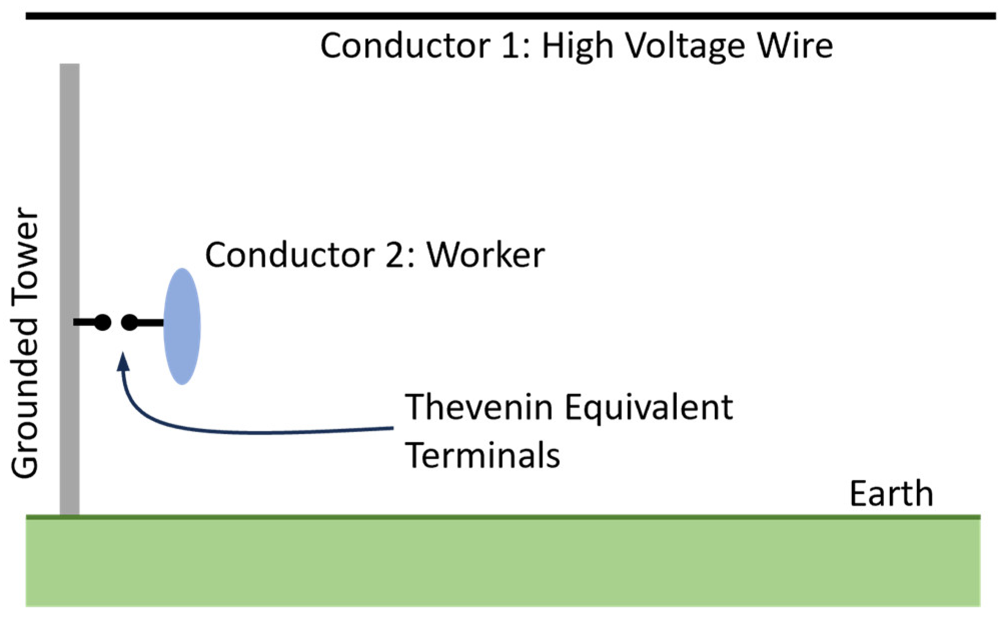
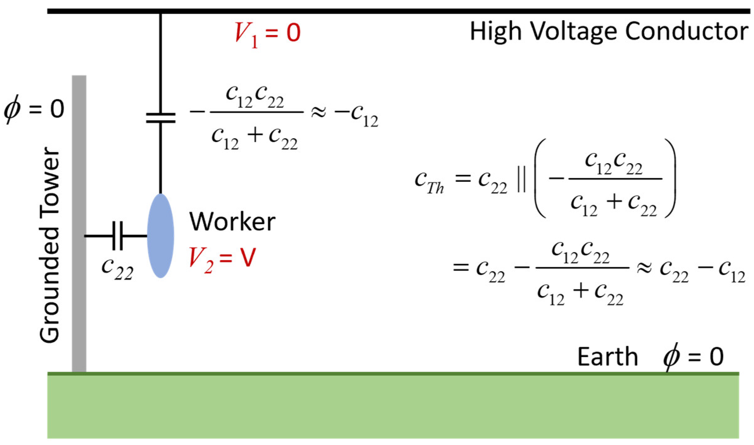
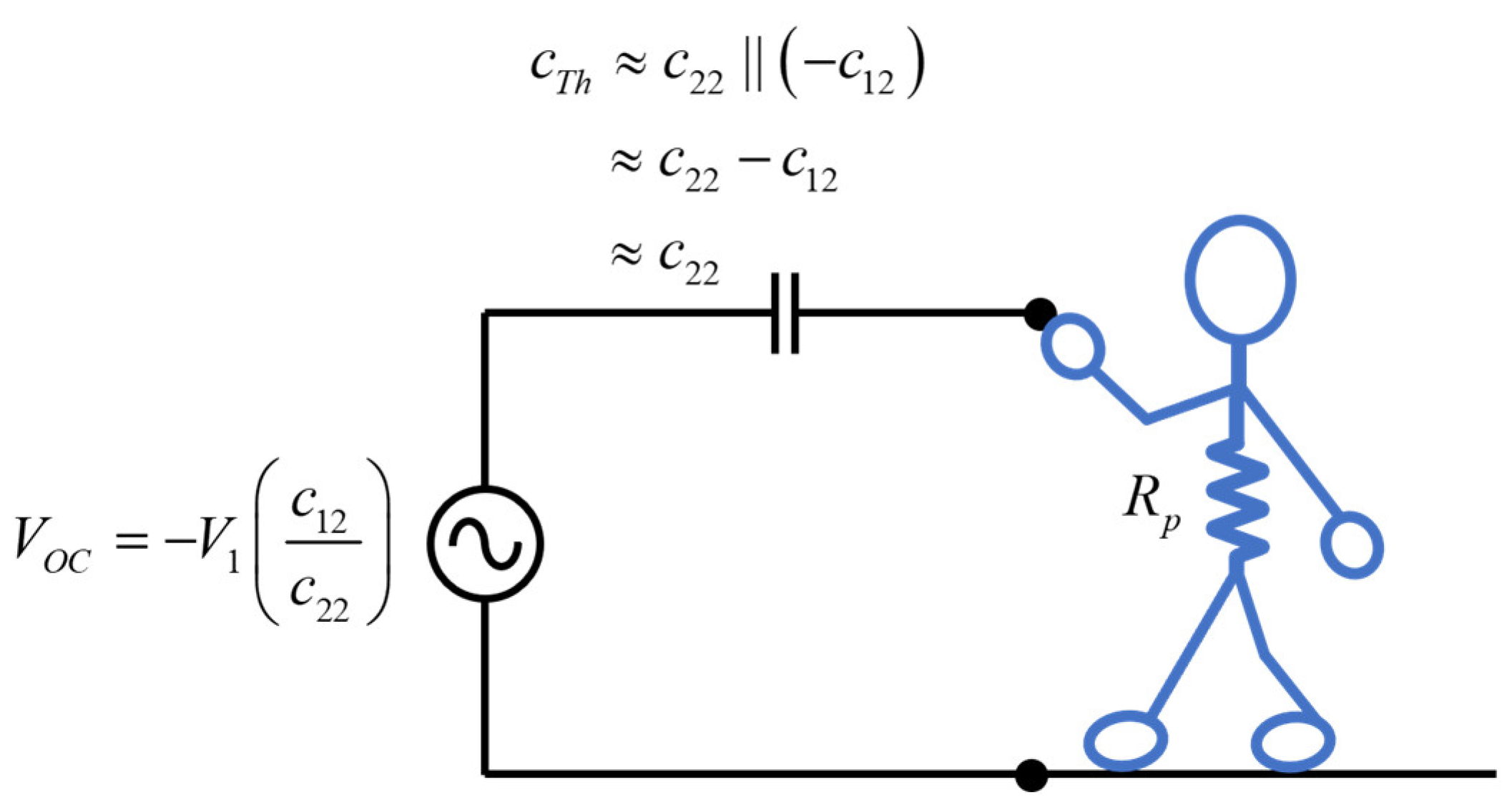
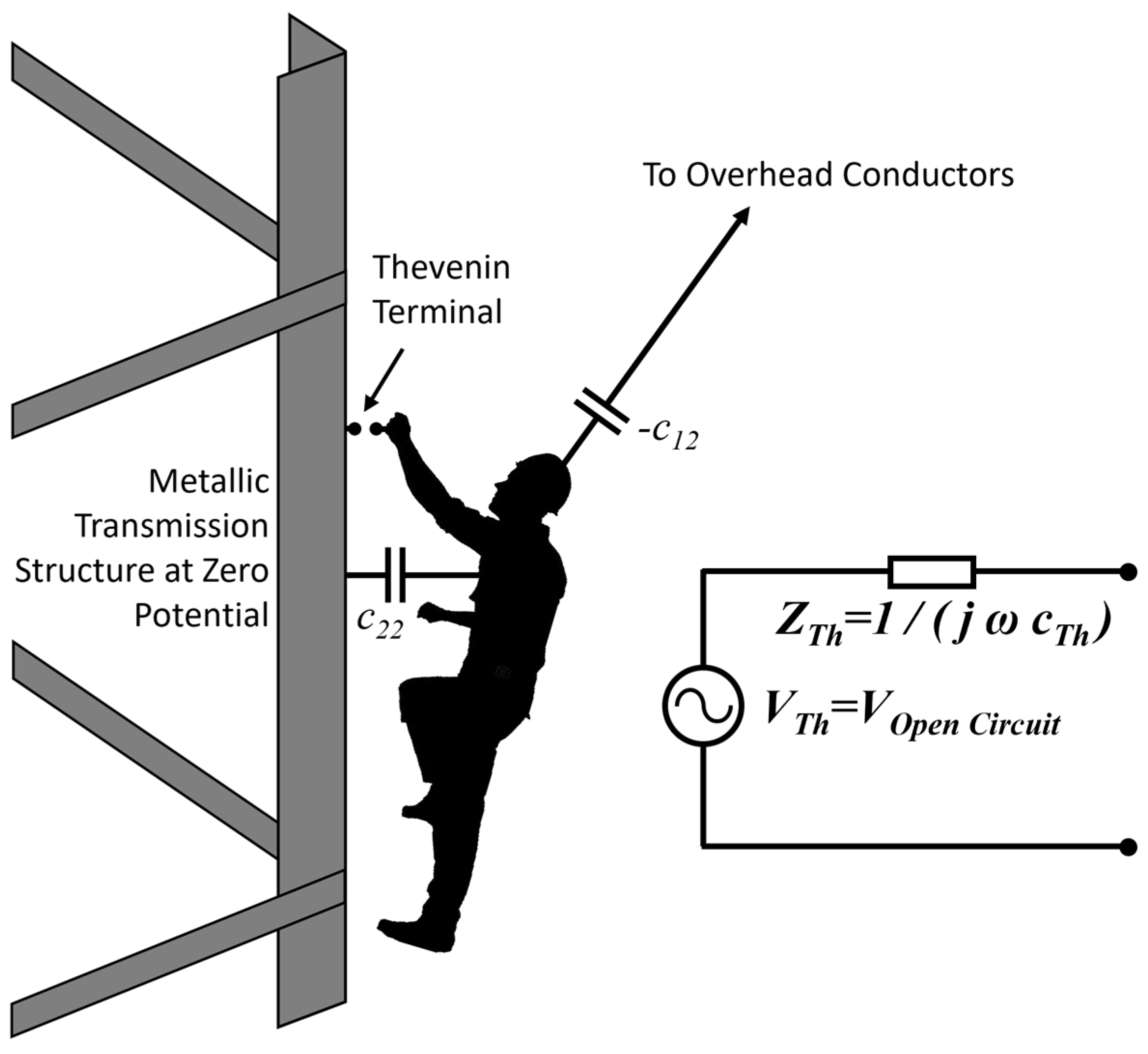
2.1. Application of Thevenin’s Theorem to the Case of High-Voltage Workers

The geometry of the problem is illustrated in Figure 1. Here, a worker (represented by a spheroid and assumed to be insulated from the tower) is climbing a tower near a high-voltage conductor energized to an AC voltage. As a result, there is a difference in voltage between the worker and tower that can lead to a microshock when the worker makes non-insulated contact with the tower. It will be assumed here that the high voltage conductor, the tower, the earth, and the worker are perfect conductors and that the fields can be analyzed using quasi-electrostatics. The goal is to develop a Thevenin equivalent circuit for the entire system at the terminals indicated in Figure 1. The current calculated for a short circuit across these terminals is both the current for the grounded condition and the driving force behind microshocks for the transient condition.

The background for the analysis that follows can be found in [20]. First, it will be assumed that the tower and the earth are held at zero potential (i.e., $\varphi =0$). Given this, the charge on the high-voltage conductor (conductor #1) or the worker (conductor #2) can be found by splitting the problem into two (since the problem is linear and superposition holds) and solving Laplace’s equation for each problem. These equations are:

$${\nabla }^2{\varphi }_i=0$$

(1)

where ${\varphi }_i$ is the per-unit electric potential at a point in space due to the charge on the ith conductor.

$${\varphi }_i=1, \mathrm{on} \mathrm{conductor}$$

(2)

$${\varphi }_i=0, \mathrm{on} \mathrm{all} \mathrm{other} \mathrm{conductors}$$

(3)

Given the solutions to these problems, the total potential at any point in space is:

$$\varphi =V_1{\varphi }_1+V_2{\varphi }_2$$

(4)

where V₁ and V₂ are the voltages assigned to conductors 1 and 2, respectively. Given (4), the total charge carried by conductor i, $q_i$, can be found by applying Gauss’s law:

$$q_i=-{\epsilon }_{air}{\displaystyle \underset{S_i}{\int }\frac{\partial \varphi }{\partial n}}dS=V_1\left(-{\epsilon }_{air}{\displaystyle \underset{S_i}{\int }\frac{\partial {\varphi }_1}{\partial n}}dS\right)+V_2\left(-{\epsilon }_{air}{\displaystyle \underset{S_i}{\int }\frac{\partial {\varphi }_2}{\partial n}}dS\right)$$

(5)

where $S_i$ is the surface of the ith conductor and ${\epsilon }_{air}$ is the permittivity of air which is approximately equal to the permittivity of free space. Note that the permittivity of air changes very little with temperature, pressure, humidity, and particulate over the range of expected environmental conditions of live-line work, especially near nominal power frequencies [21,22,23]. The result in (5) holds since the boundary condition on a perfect conductor is:

$$\overline{D}\cdot {\overline{a}}_n={\epsilon }_{air}\overline{E}\cdot {\overline{a}}_n=-{\epsilon }_{air}\frac{\partial \varphi }{\partial n}={\rho }_s$$

(6)

where ${\overline{a}}_n$ is the outward normal to the surface of the conductor and ${\rho }_s$ is the surface charge density on the conductor. Given the result in (5), the total charge on each conductor can be written as a set of capacitance values as:

$$q_1=c_{11}{V}_1+c_{12}{V}_2$$

(7)

$$q_2=c_{21}{V}_1+c_{22}{V}_2$$

(8)

where c₂₁ = c₁₂ by reciprocity. The mutual capacitance terms represent the ratio of charge induced on one conductor due to the voltage on another conductor and are negative since charges of opposite polarity are induced [24]. The negative sign inherent in the mutual capacitance terms is not explicitly shown in (7) and (8), nor is it explicitly shown in subsequent equations. Similarly, image terms are not explicitly shown but calculated charges and capacitances must include them due to the presence of earth and the grounded tower. Defined in integral form, the above capacitances are:

$$c_{11}=-{\epsilon }_{air}{\displaystyle \underset{S_1}{\int }\frac{\partial {\varphi }_1}{\partial n}}dS$$

(9)

$$c_{12}=c_{21}=-{\epsilon }_{air}{\displaystyle \underset{S_{12}}{\int }\frac{\partial {\varphi }_1}{\partial n}}dS=-{\epsilon }_{air}{\displaystyle \underset{S_{21}}{\int }\frac{\partial {\varphi }_2}{\partial n}}dS$$

(10)

$$c_{22}=-{\epsilon }_{air}{\displaystyle \underset{S_2}{\int }\frac{\partial {\varphi }_2}{\partial n}}dS$$

(11)

Next, consider two special cases of Figure 1. The first is illustrated in Figure 2. Here, the high-voltage conductor (conductor #1) is held at a voltage V₁ = 1.0 per unit and the worker (conductor #2) is floating with an unknown potential V₂ and a total charge of zero.

The purpose of this problem is to determine the unknown potential of the worker which (since the potential of the tower is 0) is then the open-circuit voltage of the Thevenin equivalent circuit. This can be performed by solving Laplace’s equation for the problem of Figure 2 with the total charge on the worker set to zero. However, it is also illustrative to consider how (8) can be used. Since $q_2$ = 0, (8) reduces to:

$$0=c_{12}{V}_1+c_{22}{V}_2$$

(12)

so that

$$V_2=(-c_{12}/c_{22})V_1$$

(13)

This suggests that a capacitive voltage divider can be used to calculate the open-circuit voltage if the capacitances are known. c₂₂ and −c₂₁ are, respectively, the capacitance between the worker and the tower/earth combination and the approximate capacitance between the high voltage conductor and the worker. Such a circuit is shown in Figure 3.

A second special case of Figure 1 is illustrated in Figure 4. Here, the potential of the high-voltage conductor is set to zero and the potential of the worker is set to an arbitrary voltage V. The worker’s charge in this problem can be solved directly using Laplace’s equation. Again, insight can be gained by applying (8) to the result. More specifically:

$$q_2=c_{22}V$$

(14)

Hence,

$$c_{22}=q_2/V$$

(15)

By examination of Figure 4, the Thevenin impedance can be determined by setting the source voltage to zero (V₁ = 0) and calculating the impedance to the set of grounded conductors. The result is:

$$c_{th}\approx c_{22}\parallel (-c_{12})\approx c_{22}-c_{12}$$

(16)

where (c₂₂ − c₁₂) > c₂₂ because c₁₂ is negative and c₂₂ >> |c₁₂| because of the worker’s proximity to the tower.

Note that c₂₂ is now known and the value V₂ was calculated by solving Laplace’s equation for the geometry of Figure 2. Further, the value of c₁₂ is available from (13) since V₁ = 1 for the calculation. These results are summarized in the Thevenin equivalent circuit shown in Figure 5. Note that R_p is the resistance of the person (roughly 1500 Ohms) and can generally be neglected compared to the Thevenin impedance (i.e., $1/\left(j\omega (c_{22}-c_{12})\right)$) at the frequencies of interest. Finally, note that, since $\left|c_{12}\right|<<c_{22}$, the open-circuit voltage is much lower than the voltage on the high-voltage conductor.

2.2. Numerical Approach for Realistic Systems

Simplified cases such as that in the previous subsection serve to illustrate the theory and sometimes allow direct computation with analytical methods. Computations for more realistic situations involving complex worker or object models, tower geometry, and bundled, multi-phase conductors normally require numerical methods. The Fourier-enhanced charge simulation method [16] was selected as the primary computation method for this analysis. This is an efficient adaptation of the standard charge simulation method for three-dimensional electrostatic calculations involving infinitely long parallel conductors near finite-shaped conducting objects. While phase conductors are not actually infinite in length, modeling them as such is a very good approximation for local electric field calculations. The axial line charge densities that represent phase subconductors are each decomposed into a uniform charge density component and a nonuniform charge density component. The nonuniform components consist of line charge density segments, each with a linearly varying charge density. The finite conducting objects are modeled with a group of point charges offset from surface potential points. A typical problem involves solving for the line charge densities and point charge values given the system geometry and voltage boundary conditions. The method applies Fourier principles to reduce computational burden by moving the portions of the problem relating to conductor nonuniform line charge density to the spatial frequency domain using a discrete Fourier transform. Computation time can be significantly reduced relative to the standard all-spatial charge simulation, boundary element, or finite element methods. The overall simulation approach involves the steps listed below. These steps follow the approach described in [16,18], but with the space charge points replaced by the worker and structure charge distributions.

• Discretize the surface of finite conducting objects (conductors, worker, and structure) by selecting a set of points distributed on their surfaces. Known voltages are enforced at these points. Higher point density allows greater accuracy but at the cost of greater computational burden. These voltage match points must be distributed based on the nature of the geometry and expected relative electric field strength. For example, smaller geometric shapes for which surface electric fields are expected to be higher may require a denser point distribution than areas of larger geometry with smaller electric fields.
• Place point charges strategically at locations inside the object. Point charges are equal in number to the surface voltage match points and each charge point location is offset in a direction normal to the surface at its respective voltage match point. The offset distance from a surface voltage match point to its corresponding charge point is based on best practices for charge simulation but is usually about 1.5 to 2.0 times the longest distance from the respective surface voltage match point to the nearest adjacent surface voltage match points. If the number of point charges differs from the number of surface voltage match points, iterative optimization-based solution methods are needed.
• Select Fourier parameters that control spatial discretization of the conductor line charge density segments.
• Compute the line charge densities of each subconductor and the point charge values at each charge point that will satisfy the electric potential boundary conditions defined at the surfaces of the objects and phase conductors. Floating potential conditions require that a zero net charge limit be enforced on the applicable object(s) (in this case, the worker).
• Once the point charge values are identified, the electric potential can be accurately calculated anywhere in the insulating medium external to or at the surface of the conductors.

The above steps were applied to find line worker charge and voltage which are necessary for calculation of the Thevenin equivalent circuit components. About 6000 line charge density segments were used to model the conductors and about 10,000 points were used to model the steel pole and worker. Each simulation was solved in about one minute on a computer with a CORE i7 intel^® processor and 32 GB of RAM. Detailed timing comparisons with the finite element method are included in [16].

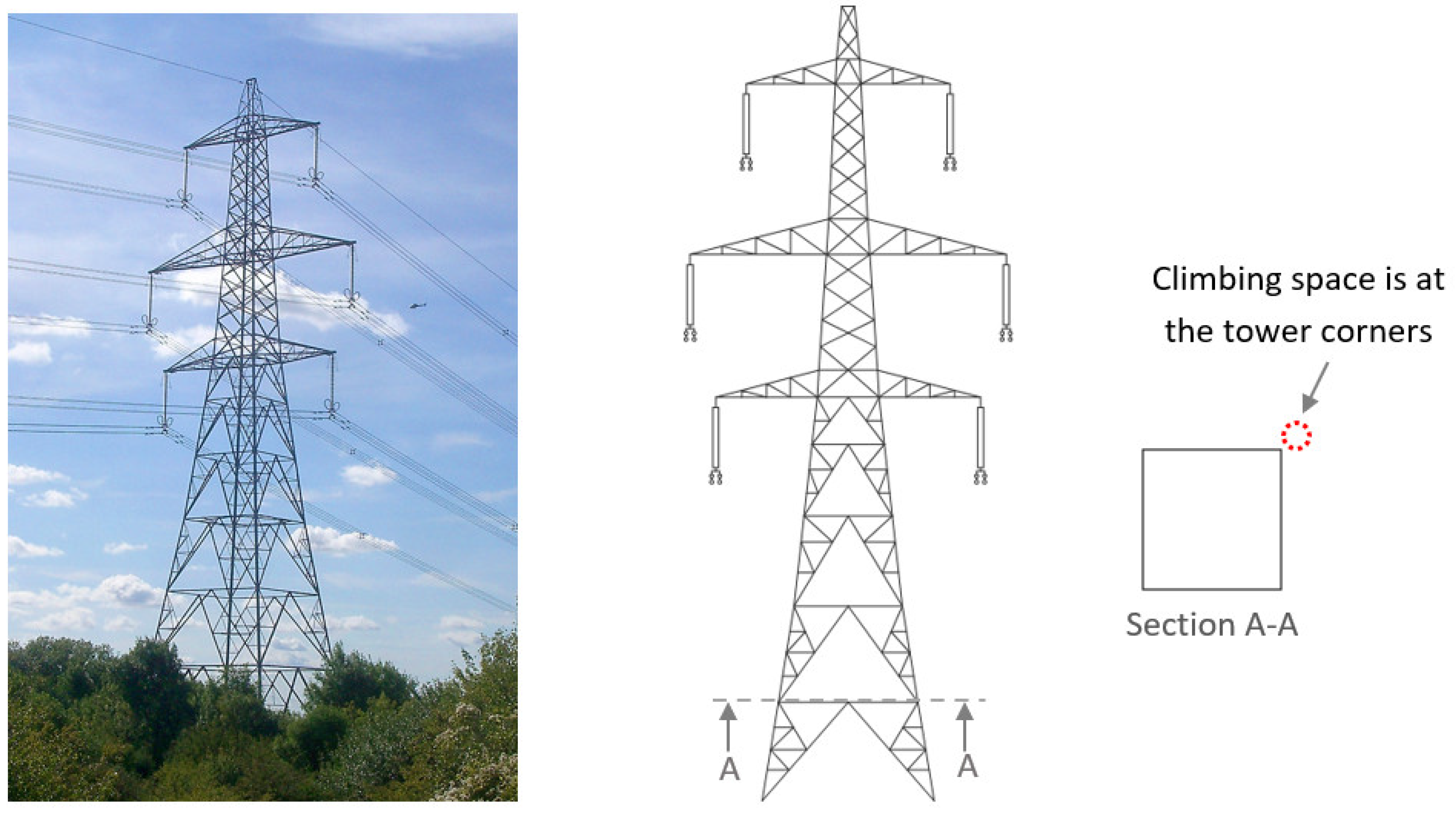
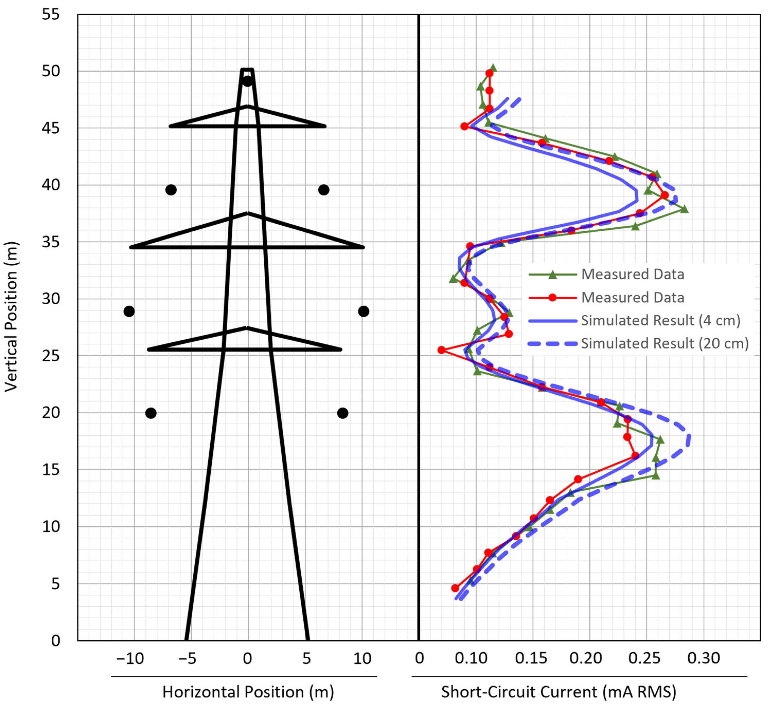
2.3. High-Voltage System Selected for Analysis

Figure 6 shows the double circuit tower used for detailed analysis and comparison to measurement. The structure is an L6 Standard D tower used in the United Kingdom. Dimensions of this and similar towers can be found in [25]. The phase conductors are located at heights of 20, 28, and 36 m, respectively, above the earth and at distances (from top to bottom) from the center of the tower of +/−6.5, +/−10, and +/−8.5 m. Each conductor is a quad bundle with subconductors of 28.63 mm diameter and 305 mm spacing. For each calculation, the conductors were set to a voltage of 400 kV rms line-to-line with reverse phasing on the two sides (i.e., ABC or RST on the left and CBA or TSR on the right).

The climbing path for these structures is along the corner legs of the towers such that the worker would be positioned facing toward the center of the tower. Even with the capabilities of modern numerical methods, modeling a detailed lattice tower is difficult and time-consuming. As a preliminary step for short-circuit computations, finite element analysis (FEA) was conducted to determine if lattice towers could be reasonably simplified to planar geometries. Figure 7 shows the two geometries analyzed. Figure 7a is a detailed lattice tower representation using flat conducting members arranged in a pattern similar to that of the L6 Standard D lattice tower, but without the taper. The model in Figure 7b has the same outer dimensions but consists of conducting planar surfaces. Both models include a single tubular conductor (not shown) with radius equal to the geometric mean radius of the L6 Standard D conductor bundle. This equivalent conductor was placed at a height and horizontal position similar to that of the lowest bundle of the L6 Standard D tower. Modeling many small-diameter conductors adds significant computational burden to the finite element model and the equivalent single conductor provides an adequate representation of the driving electric field in the region of the climbing space at the tower corner.

The tower models and earth plane were set to zero volts and the surface of the conductor was assigned a voltage of 230.9 kV rms line-to-ground. The space potential was then calculated in the region of the climbing space. Results in Figure 8 indicate that the planar model can be used without sacrificing significant accuracy. Figure 9 shows the final tower model used for the short-circuit calculations.

2.4. Human Model

Figure 10 shows the human models used for the analysis. An anthropometric model of average size was adapted from [26] and has a nominal height of about 1.8 m and a surface area of about 1.9 m². Various cases were run with model sizes ranging between ±20% of nominal based on surface area. Two other simplified shapes were used to assess the sensitivity of the method to the geometry of the line worker. These included a sphere and another shape that was simple to construct but which has proportions similar to the detailed model. The two simplified models were sized to have the same surface area as the detailed model.

Figure 11 shows an example of surface discretization for the detailed human model. The Salome program version 9.11 (https://www.salome-platform.org/, accessed 16 November 2023) was used to generate a surface mesh for the non-transmission conductor model components. The mesh is refined around areas of smaller geometry, particularly in areas where electric field will be higher. Each node of the mesh becomes a voltage control point for the charge simulation algorithm. Charge points are internal to the model at locations offset in the normal direction from the nearest charge point.

2.5. Simulation Process

Figure 12 illustrates the overall model used in the simulation process. The worker is in the climbing space and is assumed to be insulated from the phase conductors, from the grounded structure, and from reference earth by air and clothing. A Thevenin terminal is shown at a point on the worker that could come directly into contact with a grounded tool or the structure. However, selection of a specific Thevenin terminal location is not a necessary step in the process. Conduction currents through air are neglected due to air’s high resistivity. Displacement current will exist due to capacitance between the worker and the other conductors in the system, namely, the structure and ground plane, and the energized conductors. The influence of each phase conductor or phase bundle could be represented by a separate capacitance, but, for illustration simplicity, −c₁₂ is assumed to represent the net field effect of all phase conductors at the location of the worker. The structure is at ground potential but is modeled explicitly, whereas the impact of the earth plane is accounted for through image theory, assuming earth is a perfect conducting half-space.

Analysis Steps

Determination of steady-state short-circuit currents involves application of Thevenin’s theorem. First, the open-circuit voltage of the worker is determined, then the applicable Thevenin equivalent impedance is calculated, and, finally, the Thevenin circuit is used to calculate the short-circuit current. The first two steps are performed via electric field theory using the Fourier-enhanced charge simulation method.

• Step 1: Calculate the open-circuit voltage.

The open-circuit voltage (V_OC) of the worker is determined by applying a floating potential condition to the worker model when situated at a location of interest and not contacting the structure or a grounded tool. Phase conductors are energized to the desired voltage (typically the nominal voltage or the maximum operating voltage). The worker is insulated from the grounded structure and energized phase conductors, but, since the worker is in a relatively strong electric field, they will be at some non-zero potential.

Considered from the circuit perspective, the worker open-circuit voltage is based on a voltage divider between −c₁₂ and c₂₂. In this configuration, current is through the capacitances; however, it is limited by the very small value of −c₁₂.

• Step 2: Calculate the Thevenin impedance.

The next step is to find the equivalent impedance looking back into the Thevenin terminals. Following the standard Thevenin approach, voltage sources are set to zero volts. This places the capacitances in parallel, which means the equivalent impedance is due to the summation of c₂₂ (between the worker and ground) and −c₁₂ (between the worker and the conductors).

Therefore, total capacitance can be obtained by setting the conductor voltages to zero, assigning an arbitrary voltage to the worker (V_worker), calculating the corresponding total charge (Q_worker) on the worker using charge simulation, and then calculating total capacitance as C_Th = Q_worker/V_worker. The Thevenin equivalent impedance is then calculated as Z_Th = 1/(j ω c_Th), where ω is the system frequency in radians per second.

• Step 3: Calculate the short-circuit current.

The short-circuit current magnitude (I_SC) is calculated as |I_SC| = |V_OC/Z_Th| = |V_OC ω c_Th|. Use a root-mean-square (rms) voltage input to obtain an rms value for the short-circuit current. Likewise, using an AC peak voltage will give the AC peak short-circuit current.

2.6. Measurement Method

A comprehensive set of measurements performed in the UK have been provided by EPRI. The measurements covered how the short-circuit currents between a grounded line worker (linesman) and the tower vary within the normally accessed climbing space on a tower for a range of tower designs from two different tower families. The measurements were conducted on three variants of the L6 tower family (including that of Figure 6) and two variants of the L2 tower family. These variants were a tangent suspension tower (with no angle deviation of the line), a tower for line angle deviations of between 30° and 60°, and a tower for line angle deviations of between 0° and 30° for one of the tower families.

Two line workers were equipped with a logging current-measuring meter that was capable of recording event markers. This meter was used to record steady-state currents (see State 2 in Table 1). Typical accuracy of the meters is ±5%. One side of the meter was connected to the linesman’s arm by a wrist strap, tightened to ensure good contact. The other side was connected to a clamp for making electrical connections to the tower. The linesmen wore boots with resistance sufficient to make short-circuit current in paths outside the measurement strap negligible.

The two line workers climbed each tower along two climbing legs on opposite corners of the tower, starting immediately above the anti-climbing guard and climbing all the way to the very top, stopping every 5 feet (1.52 m) to make a measurement.

Step-bolts are 1 foot 3 inches apart (0.38 m), located alternately on the two sides of the angle girder of the climbing leg. The meter was recording current continuously and the linesmen were asked to stop at every second pair of step-bolts, (that is, every 5 feet or 1.52 m), fasten a non-conductive work position strap around the tower leg, lean back into it with no other contact with the tower, and take a current reading by recording an event mark on the current-logging meter. The distance from the tower to the closest point on the worker was estimated to be between bounds of 4 cm and 20 cm. Two observers on the ground, one for each linesman, recorded the locations of their feet for each event number. The height of each line worker was within 10% of a reference height of 5.77 feet (1.76 m). Body mass index was also recorded for each line worker and their surface areas were estimated to be similar to a reference value of 20.5 square feet (1.90 square meters), similar to the size of the nominal human model used in simulation.

Only the results for the L6 D Standard tower are included in this paper for comparison to calculated values. A full set of measured data for the other tower families will be incorporated in a forthcoming EPRI report.

The measurement process took place a couple of years before the simulation work for this research. Since measurement and simulation were not originally part of the same experiment design, some detailed information was unavailable to the authors of the present paper. Notably, the exact volume and surface area of the linesman are unknown so physical comparison was based primarily on the height and description of build. Moreover, the specific tower corner climbed by each of the linesmen is unknown. This could have some impact on results due to the asymmetrical phasing arrangement. However, the phases closest to the respective climbing path would dominate. Consequently, neither of these issues was expected to introduce significant error.

3. Results

Calculated and measured results for the short-circuit current between the insulated worker and the tower as a function of the worker vertical position along the corner leg climbing path of the L6 D Standard tower are given in Figure 13. One measured dataset is shown for each of the two workers who climbed the tower as described in Section 2.3 and Section 2.6. The two simulated datasets are both for the same detailed human model in Figure 10a, but one has a 4 cm gap between the tower surface and the closest part of the model (the feet) and the other has the model placed at a distance of 20 cm from the tower surface.

Table 2. Mean percentage error calculations.

		Simulated Results
		4 cm Spacing	20 cm Spacing	Average
Measured Results	Linesman 1	8.14%	−8.53%	−0.19%
	Linesman 2	3.30%	−14.5%	−5.59%
	Average	6.45%	−10.6%	−2.08%

Note: The row and column header for each result in Table 2 indicates the two datasets used for the respective MPE calculation. For example, the MPE for the measured results for Linesman 2 and the simulated results for the case with 4 cm spacing to the tower is 3.3%.

lists the mean percentage error (MPE) values calculated for the measured datasets compared to the simulated datasets. Prior to calculating MPE, linear interpolation was applied to each dataset to generate short-circuit current arrays on regular vertical position intervals. Rows and columns labeled “Average” involve MPE computation on an array of data calculated as a point-by-point average of the respective measured or simulated results. MPE values in the “Average” column are relatively small, which is reasonable since the 4 cm and 20 cm spacings for calculated results represent the estimated bounds of linesman closest distance to the tower. Overall, error values are reasonable given the data available about the measurement process.

Table 3. Comparison of short-circuit currents for varying human model size.

Human Model Size * (Percent of Surface Area Relative to the Nominal Case)	Open-Circuit Voltage (Volts rms)	Model Capacitance (Picofarads)	Short-Circuit Current (Milliamperes)	Space Potential without Model (Volts rms)
80%	7900	67.1	0.167	8085
90%	8239	71.1	0.184	8449
100%	8562	74.7	0.201	8808
110%	8841	78.4	0.218	9156
120%	9118	81.9	0.235	9486

* Models were placed 4 cm from the tower surface. The detailed model from Figure 10a was used.

lists the results of the simulations to analyze the impact of line worker size on short-circuit currents. Worker models for these cases were placed 4 cm from the surface of the tower corner at a vertical location corresponding to the worst-case short-circuit current.

Table 4. Comparison of simulation results for three human model shapes (refer to Figure 10a).

Model *	Open-Circuit Voltage (Volts rms)	Model Capacitance (Picofarads)	Short-Circuit Current (Milliamperes)	Space Potential without Model (Volts rms)
Sphere	11,538	64.2	0.233	12,817
Human analog	11,881	64.2	0.240	12,358
Detailed human	11,916	63.0	0.236	11,937

* Models were placed 20 cm from the tower surface. As expected, this results in higher open-circuit voltages than the cases in Table 2 which were placed closer to the tower.

compares results for the three worker model shapes. Worker models for these cases were placed 20 cm from the surface of the tower. The last column in both tables shows the space potential calculated at approximately the volumetric center of the human model, but without the model present (i.e., only the structure, ground, and energized conductors are in the model). This is for comparison to the open-circuit voltage.

The results for open-circuit voltage, model capacitance, and short-circuit current each vary approximately linearly with model surface area. The changes in capacitance and short-circuit current are not drastic for any of the cases in Table 3 and Table 4. Moreover, the space potential calculated in the absence of the model is close to the open circuit voltage. These suggest that a reasonable rule-of-thumb estimate of short circuit could be obtained by assuming a typical value of capacitance and estimating the space potential in the climbing space. The fact that there is little difference in the results for the three models with the same surface area indicates that results are not sensitive to shape of the line worker.

4. Discussion

The Fourier-enhanced charge simulation method was well-suited for an analysis of the line worker short-circuit problem and provides insight which could help facilitate research into mitigation methods. The key assumptions or simplifications are the use of horizontal conductors, the discretization of the geometry, and the size and placement of the human model. These are typical concessions for most numerical-based methods. The proposed method has the advantage of easily accommodating a detailed human model and explicitly modeling each of the subconductors in the phase bundles. Results compare well with measured values, indicating the simulation method could be used by utilities to calculate the steady-state induced short-circuit current, which is one key determinant of microshock severity. Access to practical short-circuit calculation methods and results would allow utilities to better prepare line workers for the severity of microshocks to which they could be exposed. It could also be used to quickly identify situations that would result in currents above safety thresholds established by utilities.

Compared to the detailed human model, relatively little error was introduced using the simplified human shape or the spherical human analog. This suggests that certain sensitivity studies could be performed using very simplified worker geometry with an equivalent surface area. This makes sense given that the electric field does not change drastically in the climbing space within volumes that would be occupied by a worker.

While detailed simulation and measurement tend to produce the most accurate results, a quick estimate of maximum worker-induced short-circuit current can be obtained through reasonable assumptions regarding the Thevenin capacitance (c_Th) and the open-circuit voltage (V_OC). The short-circuit current can then be estimated as I_sc = V_OC ω c_Th, where ω is the system frequency in radians per second. Note that worker size and the distance to the surface of the grounded structure being climbed will generally vary over relatively narrow ranges. Therefore, c_Th will also fall in a relatively narrow range. Moreover, as previously mentioned, the high-voltage conductors have a relatively minor impact on worker Thevenin capacitance. Therefore, based on the data in Table 3 and Table 4 and the results in the example of Figure 13, the Thevenin capacitance of the average-sized worker can be estimated to be between about 65 pF and 80 pF depending on the proximity to the surface of the structure. Use of the higher end of the range would typically be best for purposes of estimating induced short-circuit current. The open-circuit voltage without the worker present can then be estimated using (19) from [27]. This is the equation for the space potential at some distance from an energized conductor near a perfect conducting ground plane which replaces the lattice tower structure. The parameters of the equation are illustrated in Figure 14. Note that the approach neglects two of the phases. Inclusion of the other phases during balanced operating conditions introduces partial field cancellation which would reduce the calculated open circuit voltage.

Table 5. Estimate of short-circuit current calculated by applying (19) to the example of Figure 13.

Parameter	Value	Comment
a	0.137 m	GMR for a quad bundle with spacing of 0.305 m and subconductor diameter of 2.861 cm, calculated using standard equations in [2].
d	0.44 m	Human model is about 0.3 m in depth. Average distance from the front of the person to the tower surface is about 14 cm (4 cm at the feet with a tower surface slope of about 8:1 at the height of the lowest conductor).
h	5.26 m	Approximately 5.7 m from the center of the lowest bundle to the surface of the tower.
VLG	230.94 kV	400 kV line-to-line nominal voltage (rms) at a frequency of 50 Hz.
VOC	8075 Volts	Volts rms calculated using (19).
cTh	80 pF	The high end of the suggested range.
Ishort-circuit	0.203 mA rms	Compare to the maximum simulated result of 0.204 mA rms.

lists the parameters and results of applying (19) to estimate the maximum short-circuit current for the example illustrated in Figure 13. The accuracy of the estimate in this case is somewhat coincidental but would typically be within 10 or 15% of the simulated case.

$$V_{OC}=\frac{V_{LG}}{\ln \left(2\left(h+d\right)/a\right)}\ln \left(\frac{h+2d}{h}\right)$$

(17)

References

1. Keesey, J.C.; Letcher, F.S. Minimum Thresholds for Physiological Responses to Flow of Alternating Electric Current Flow through the Human Body at Power-Transmission Frequencies; Project MR005.8-0030B; Naval Medical Research Institute: Bethesda, MD, USA, 1969. [Google Scholar]
2. International Commission on Non-Ionizing Radiation Protection. ICNIRP guidelines for limiting exposure to time-varying electric and magnetic fields (1 Hz to 100 kHZ). Health Phys. Soc. 2010, 99, 818–836. [Google Scholar] [CrossRef] [PubMed]
3. Swanson, D.W.; (Bonneville Power Administration, Portland, OR, USA). Private Communication, 2023.
4. Ahmed, Y.; Rowland, S.M. UK Linesmen’s Experience of Microshocks on HV Overhead Lines. J. Occup. Environ. Hyg. 2009, 6, 475–482. [Google Scholar] [CrossRef] [PubMed]
5. IEEE. 2023 National Electrical Safety Code® (NESC®); IEEE: Piscataway, NJ, USA, 2022. [Google Scholar]
6. Pan, W.; Li, X.; Li, Y. Calculation and Analysis of Micro-Shock Energy of Line Maintenance Personnel in High Electric Field. In Proceedings of the 5th Asia Conference on Power and Electrical Engineering (ACPEE), Chengdu, China, 4–7 June 2020. [Google Scholar]
7. Lu, T.; Li, X. Measurement of Electrostatic Discharge Through Human Body Contacting Metallic Objects Under HVAC Transmission Lines. In Proceedings of the 41st Annual EOS/ESD Symposium (EOS/ESD), Riverside, CA, USA, 15–20 September 2019. [Google Scholar]
8. He, W.; Zhang, Y.; Liu, Y.; Chen, Q.; Han, X.; Zhou, D.; Wei, H.; Wan, B. Experimental Study on the Transient Electric Shock Characteristics Between Metal Sheds and the Human Body Near Ultrahigh Voltage Alternating Current Transmission Lines. IEEE Trans. Electromagn. Compat. 2023, 65, 679–688. [Google Scholar] [CrossRef]
9. Ahmed, Y.; Rowland, S.M.; Burnett, G.; Pammenter, N. Avoidance of Microshocks for HV Overhead Line Workers. In Proceedings of the International Conference on Electric and Magnetic Fields at Extremely Low Frequencies, Paris, France, 24–25 March 2011. [Google Scholar]
10. Martinsen, Ø.G.; Grimnes, S.; Piltan, H. Cutaneous Perception of Electrical Direct Durrent. ITBM-RBM 2004, 25, 240–243. [Google Scholar] [CrossRef]
11. Prausnitz, M.R. The Effects of Electric Current Applied to Skin: A Review for Transdermal Drug Delivery. Adv. Drug Deliv. Rev. 1996, 18, 395–425. [Google Scholar] [CrossRef]
12. Gunatilake, A.; Ahmed, Y.; Rowland, S.M. Modelling of Microshocks Associated With High-Voltage Equipment. IEEE Trans. Power Deliv. 2009, 24, 202–207. [Google Scholar] [CrossRef]
13. Ahmed, Y.; Rowland, S.M. Modelling Linesmen’s Potentials in Proximity to Overhead Lines. IEEE Trans. Power Deliv. 2009, 24, 2270–2275. [Google Scholar] [CrossRef]
14. Lin, C.J.; Chuang, R.; Chen, M. Steady-state and Shock Currents Induced by ELF Electric Fields in a Human Body and a Nearby Vehicle. IEEE Trans. Electromagn. Compat. 1990, 32, 59–65. [Google Scholar] [CrossRef]
15. Abdel-Salam, M.; Abdallah, H.M. Transmission-Line Electric Field Induction in Humans Using Charge Simulation Method. IEEE Trans. Biomed. Eng. 1995, 42, 1105–1109. [Google Scholar] [CrossRef] [PubMed]
16. Leman, J.T.; Olsen, R.G. Fourier Enhanced Charge Simulation Method for Electrostatic Analysis of Overhead Transmission Lines. IEEE Trans. Power Deliv. 2022, 37, 1078–1087. [Google Scholar] [CrossRef]
17. Olsen, R.G.; Leman, J.T. On Calculating Contact Current for Objects Insulated from the Earth and Immersed in Quasi-static Electric Fields. IEEE Power Energy Technol. Syst. J. 2017, 4, 16–23. [Google Scholar] [CrossRef]
18. Leman, J.T.; Olsen, R.G. On Calculating the Phase-to-Phase CFO of Overhead Transmission Lines Based on the Spatial Minimum Electric Field. IEEE Trans. Power Deliv. 2022, 37, 3698–3708. [Google Scholar] [CrossRef]
19. Co, G.E. Transmission Line Reference Book—345 kV and Above, 2nd ed.; Electric Power Research Institute: Palo Alto, CA, USA, 1982. [Google Scholar]
20. Bladel, J.V. Electromagnetic Fields, 2nd ed.; Wiley-IEEE Press: Hoboken, NJ, USA, 2007. [Google Scholar]
21. Choi, J.M.; Kim, T.W. Humidity Sensor Using an Air Capacitor. Trans. Electr. Electron. Mater. 2013, 14, 182–186. [Google Scholar] [CrossRef]
22. Salas-Sánchez, A.; Rauch, J.; López-Martín, M.; Rodríguez-González, J.; Franceschetti, G.; Ares-Pena, F. Feasibility Study on Measuring the Particulate Matter Level in the Atmosphere by Means of Yagi-Uda-Like Antennas. Sensors 2020, 20, 3225. [Google Scholar] [CrossRef] [PubMed]
23. Li, T.; Lin, Q.; Chen, G. Live-Line Operation and Maintenance of Power Distribution Networks; China Electric Power Press: Beijing, China, 2017. [Google Scholar]
24. Morrison, R. Digital Circuit Boards: Mach 1 GHz; John Wiley & Sons: Hoboken, NJ, USA, 2012. [Google Scholar]
25. Beardsmore, D. L6–Telcontar.net. Available online: https://telcontar.net/Power/pylons/L6 (accessed on 31 August 2023).
26. Huysmans, T.; Molenbroek, J. DINED/Anthropometry in Design. 2023. Available online: https://dined.nl/en (accessed on 21 May 2023).
27. Olsen, R.G. High Voltage Overhead Transmission Line Electromagnetics—Volume I, 2nd ed.; CreateSpace: Scotts Valley, CA, USA, 2018. [Google Scholar]
Figure 1. Geometry of the problem.
Energies 16 07646 g001
Figure 2. Determining the open-circuit voltage of the Thevenin equivalent.
Energies 16 07646 g002
Figure 3. Determination of open-circuit voltage for the Thevenin equivalent circuit.
Energies 16 07646 g003
Figure 4. Determination of Thevenin impedance.
Energies 16 07646 g004
Figure 5. Final Thevenin equivalent.
Energies 16 07646 g005
Figure 6. UK L6 Standard D Tower. (The tower in the photo has a 20-foot extension).
Energies 16 07646 g006
Figure 7. Models used to assess required tower detail: (a) detailed lattice tower model, and (b) simplified planar surface model. Outer dimensions of both are 6.2 m × 6.2 m × 25 m.
Energies 16 07646 g007
Figure 8. Comparison of space potential along the climbing path for the models in Figure 7.
Energies 16 07646 g008
Figure 9. Simplified UK L6 Standard D tower model.
Energies 16 07646 g009
Figure 10. Human models used to calculate the Thevenin equivalent circuit: (a) detailed model, (b) simple shape with overall proportions similar to the detailed model, and (c) spherical model. All models have the same surface area.
Energies 16 07646 g010
Figure 11. Example of surface discretization of the detailed human model. Mesh nodes become voltage control points for the charge simulation algorithm. Charge points are internal to the model at locations offset from the voltage control points in a direction normal to the surface.
Energies 16 07646 g011
Figure 12. Illustration of model used for the simulation process.
Energies 16 07646 g012
Figure 13. Comparison of measured and simulated steady-state short-circuit results versus worker vertical position along the L6 D Standard tower climbing path (at the tower corners). Measured results are for each of the two linesmen described in Section 2.6. Simulated results are for the detailed human model with one set corresponding to a 4 cm separation from the tower and the other set corresponding to a 20 cm separation from the tower.
Energies 16 07646 g013
Figure 14. Simplified geometry for short-circuit current estimate using (19).
Energies 16 07646 g014