Article

A Fast Screening Method of Key Parameters from Coal for Carbon Emission Enterprises

1
School of Electric Power, South China University of Technology, Guangzhou 510640, China
2
Guangdong Institute of Special Equipment Inspection and Research Shunde Branch, Foshan 528300, China
*
Author to whom correspondence should be addressed.
Energies 2023, 16(22), 7592; https://doi.org/10.3390/en16227592
Submission received: 28 September 2023 / Revised: 1 November 2023 / Accepted: 2 November 2023 / Published: 15 November 2023
(This article belongs to the Section B3: Carbon Emission and Utilization)

Abstract

:
During the process of determining carbon emissions from coal using the emission factor method, third-party organizations in China are responsible for verifying the accuracy of the carbon emission data. However, these verifiers face challenges in efficiently handling large quantities of data. Therefore, this study proposed a fast screening method that utilizes multiple linear regression (MLR), in combination with the stepwise backward regression method, to identify problematic carbon emission data for the lower calorific value (LCV) and carbon content (C) of coal. The results demonstrated the effectiveness of the proposed method. The regression models for LCV and C exhibited high R-squared (R2) values of 0.9784 and 0.9762, respectively, and the root mean square error (RMSE) values of the validation set were 0.32 MJ/kg and 0.80% for LCV and C, respectively, indicating strong predictive capabilities. By analyzing the obtained results, the study established the optional error threshold interval for the LCV and C of coal as 2RMSE–3RMSE. This interval can be utilized as a reliable criterion for judging the quality and reliability of carbon emission data during the verification process. Overall, the proposed screening method can serve as a valuable tool for verifiers in assessing the quality and reliability of carbon emission data in various regions.

1. Introduction

With the rapid development of the carbon trading market in China, the accurate determination of carbon dioxide emissions has become crucial [1,2]. The widely used emission factor method, also known as the standard calculation-based method, is utilized for calculating carbon emissions from coal combustion [3,4]. Key parameters, such as lower calorific value (LCV) and carbon content (C) per unit of calorific value, are measured to determine the carbon emissions of fossil fuels [5]. In China, these parameters are provided by carbon emission enterprises and may be inspected by third-party verifiers to ensure accuracy. Currently, verifiers rely on tracking the historical carbon emissions of enterprises as evidence for assessing their reports. However, due to the vast amount of data involved in evaluating carbon emissions, it is essential to establish an efficient screening method that can facilitate the identification of potential problematic data, particularly in coal burning processes that often require more extensive data analysis. By establishing a set of predetermined thresholds for the key parameters, it will be easier for verifiers to quickly identify whether the reported data falls within an acceptable range.
Extensive research has been conducted on the correlation between the calorific value of coal and other parameters, due to its significant impact on combustion performance and coal quality assessment. Linear regression models have been developed using proximate analysis [6,7,8,9,10,11,12,13], ultimate analysis [14], or a combination of both [11,15], as shown in Table 1. These calorific value models exhibit good predictive accuracy, with R2 values ranging from 0.97 to 0.998 and mean absolute error (MAE) values ranging from 1.45% to 3.74%. Additionally, it was observed that the combination of both analyses usually yields better results [16]. Nonlinear methods—such as artificial neural networks (ANN) [12,17,18,19], adaptive neuro-fuzzy inference systems (ANFIS) [20], support vector regression (SVR) [16,21,22], random forest (RF) [23], and so on—have also been utilized for prediction. While nonlinear methods require more data and complex training processes, linear regression remains a simple and practical approach, especially when the predictions fall within an acceptable range. Hence, linear regression is used in this study for ease of application in screening carbon emission data.
Fewer studies have specifically focused on predicting carbon content (C) in coal, potentially due to its limited correlation with coal prices. However, some regression equations for C have been developed [24,25,26,27,28], as shown in Table 1. These C models exhibit moderate predictive accuracy, with R2 values ranging from 0.86 to 0.95 and MAE values ranging from 0.51% to 1.97%. Additionally, nonlinear methods, such as partial least squares (PLS) [24,29], back-propagation neural networks (BP-ANN) [24], and support vector machines (SVM) [30,31], have also been gradually applied to predict C.
The existing models in the literature cover a wide range of fuel types and calorific values. For instance, Parikh et al.’s model covers different types of solid fuels, with dry basis gross calorific value (GCV) ranging from 14.772 to 34.388 MJ/kg [8]. Channiwala et al.’s model includes various types of solid, liquid, and gaseous fuels, with fuel dry basis GCV ranging from 4.745 to 55.345 MJ/kg [15]. Majumder et al. focused on coal samples, with received basis GCV ranging from 12.75 to 28.37 MJ/kg [9]. Consequently, existing models generally predict LCV with relatively high uncertainty, limiting their applicability as a screening method.
This study proposed a screening method based on multiple linear regression models, specifically utilizing coal samples from China. The optimal multivariate linear regression models of LCV and C were established by evaluating the significance of various coal parameters obtained from both proximate analysis and ultimate analysis. Using these models, verifiers can quickly compare the reported carbon emission data with the model’s predictions to identify any discrepancies. This method provides a reliable and efficient approach for verifiers to quickly screen carbon emission data.

2. Materials and Methods

2.1. Sample Collection and Preparation

In this research, we collected 95 coal samples from enterprises located across certain province, China. The selection of these samples was carried out in a random manner to ensure their representativeness. These parameters encompassed total moisture; moisture content; ash content; volatile matter content; and fixed carbon content, among others, all of which were determined using standardized prescribed methodologies. All measurements were executed under air-dry conditions. Additionally, the values of LCV and C were appropriately adjusted to a received basis.
The experimental findings for the coal samples are presented in Table 2. The moisture content exhibited a range from 2.48% to 19.92%, while ash content ranged from 3.69% to 34.06%. Volatile matter content spanned from 25.52% to 42.41%, while fixed carbon content varied between 34.07% and 60.74%. Total sulfur content ranged from 0.12% to 1.98%; hydrogen content from 3.23% to 4.41%; carbon content from 39.90% to 61.14%; and LCV from 14.85 MJ/kg to 22.78 MJ/kg. The predominant coal types in the region were identified as bituminous coal and lignite, characterized by generally higher volatile matter and LCV. To facilitate the analysis, the dataset of 95 coal samples was randomly split into two subsets: a calibration set and a validation set. The calibration set, comprising 85 sets of data, was employed to develop multiple linear regression models for both C and LCV. The validation set, consisting of 10 data sets, was utilized to assess the performance of the regression models.

2.2. Methodology

2.2.1. Multiple Linear Regression

Multiple linear regression is a statistical method used to explore the quantitative relationship between a dependent variable (y) and multiple independent variables (x1, x2, …, xn). This method assumes a linear relationship between the dependent variable and the independent variables. The multiple linear regression model can be expressed as follows [32]:
y = a 0 + a 1 x 1 + a 2 x 2 +   + a n x n + ε .
In this equation, a0, a1, a2, …, an are the regression coefficients that represent the impact of each independent variable on the dependent variable. The term ε represents the random error term, which captures the unexplained variability in the relationship.

2.2.2. Stepwise Backward Regression Method

The stepwise backward regression method is a useful statistical analysis method which can assist researchers in excluding independent variables that have minimal contribution to the dependent variable from the model, thereby improving the predictive accuracy of the regression model [33]. Its specific procedure is as follows: Firstly, a regression equation is established by using all m variables, and then the least significant variable among these m variables—referring to the one with the largest p-value (denoted as sig(t)) in the regression coefficient test—is selected and eliminated from the equation. A t-test is then performed on the m regression coefficients, yielding p-values denoted as {P1, P2, …, Pm}. The variable with the largest p-value is identified and denoted as:
P j = m a x   P 1 ,   P 2 ,   ,   P m   .
Given a significance level of α, if Pj ≥ α, the variable xj is first eliminated from the regression equation. Then, a regression equation is established again with the remaining m-1 independent variables, and a significance test is conducted on the regression coefficients. This process continues sequentially, until the t-test values of all remaining variables in the regression equation are less than the significance level α, indicating that no more variables can be removed. At that time, the obtained regression equation is the final determined equation.
The flow chart of the methodology of this study is shown in Figure 1. For this study, we utilized SPSS statistical analysis software to establish multiple linear regression models for C and LCV based on the 85 data sets. Then, the stepwise backward regression method was used for the selection of independent variables, including the significance test of the regression model (F-test) and the significance test of the regression coefficient (t-test). The aim was to identify the most relevant independent variables that contribute to the prediction of C and LCV. Finally, the predicted values of the model (LCV and C) can be compared with the data reported by the enterprise. If the error of the above two is greater than the preset threshold (2RMSE–3RMSE), the data is doubtful, and further analysis is required. This method is helpful for verifiers to quickly identify whether the reported data falls within an acceptable range.

2.2.3. Model Evaluation Indicators

The obtained multiple linear regression models for C and LCV were evaluated using several indicators to assess the accuracy and reliability of the models. These indicators included the R-squared (R2), the root mean square error (RMSE), the mean absolute error (MAE), and the mean relative error (MRE). The coefficient of determination (R2) indicates the proportion of variance in the dependent variable that can be explained by the independent variables. The root mean square error (RMSE) measures the average magnitude of the residuals between the predicted and actual values, providing an overall assessment of the model’s prediction accuracy. The mean absolute error (MAE) calculates the average absolute difference between the predicted and actual values, representing the average magnitude of the errors. The mean relative error (MRE) measures the average percentage difference between the predicted and actual values, indicating the average relative deviation.
Generally, smaller values of RMSE, MAE, and MRE indicate higher prediction accuracy of the model [34,35]. The values of R2, RMSE, MAE, and MRE are calculated using Formulas (3)–(6).
R 2 = 1 i = 1 n y i y ^ i 2 i = 1 n y i y ¯ 2
R M S E = i = 1 n y i y ^ i 2 n
M A E = i = 1 n y i y ^ i n
M R E = i = 1 n y i y ^ i y i n
In the equation, yi and y ^ i represent the reference values and model predictions, respectively; y ¯ represents the mean of reference values; n represents the number of coal samples; and k is the number of independent variables.

3. Results

3.1. Model Building

3.1.1. Low Calorific Value

To develop a multiple linear regression model (Model 1 as listed in Table 3) for LCV, all parameters from proximate analysis and ultimate analysis (C, H, S, M, A, V, FC) were used as independent variables. The performance of the model was assessed through analysis of variance (ANOVA), including metrics such as R2, F-test, and t-test [36].
R-squared (R2) for Model 1 was found to be 0.9775. This value indicates a strong linear fit between the independent variables and the low calorific value. The F-test, which assesses the overall significance of the regression model, yielded a significance level (Sig.(F)) of 3.53 × 10-62, which is considerably lower than the significance threshold of 0.05, indicating that the model has a significant linear relationship with LCV. However, the t-test results indicated that the variables Vad, Aad, FCad, and Had were not statistically significant (Sig.(t) > 0.05) in relation to LCV. This suggests that these parameters have an insignificant linear relationship with LCV and may not contribute significantly to the prediction of LCV within this model.
Next, the stepwise backward regression method was employed to refine and improve the predictive performance of the regression model. Starting from the independent variables of the previous regression model, the parameter with the largest value of Sig.(t) (indicating insignificance) was identified and eliminated. The remaining independent variables were then used for the subsequent regression. This process was repeated until all remaining independent variables were significant.
In this case, the parameters Vad, Aad, FCad, and Had were eliminated in sequence, as they were determined to be statistically insignificant. With each elimination, the R-squared (R2) value increased, indicating an improved fit of the model. Additionally, the significance level (Sig.(t)) of the remaining parameters decreased, indicating their increased significance in relation to LCV.
By employing the stepwise regression procedure, we generated a refined model (Model 5) that incorporates only the significant independent variables, written as:
Q n e t , a r = 1.202 0.032 M a d + 0.359 S t , a d + 0.398 C a r .
The R2 value of this model is 0.9784, indicating a slight improvement compared to the initial model. The inclusion of the parameters Mad, St,ad, and Car in the model is statistically significant, as evidenced by their Sig.(t) values being less than 0.05. This suggests a significant linear relationship between each independent variable and the dependent variable LCV.

3.1.2. Carbon Content

The multiple regression model for C was developed using the same process described above. The initial model included seven coal quality parameters (Q, H, S, M, A, V, FC), and a stepwise backward regression procedure was conducted to refine the model. The refined model for C is presented in Table 4 and written as:
C a r = 15.649 0.129 A a d 0.159 V a d + 2.228 L C V a r .
After conducting a stepwise backward regression, only three parameters were found to have a high level of significance and were retained in the model. The R2 value of 0.9762 indicated a good fit. Furthermore, the Sig.(F) value of the model, which is 2.96 × 10−66 (less than 0.05), indicates that the fitted regression equation is statistically significant and demonstrates a linear relationship between the independent variables and the dependent variable. This suggests that the selected parameters play a crucial role in predicting C accurately.
It is important to note that the models are specific to the analyzed coal samples and may not be generalized to other datasets or coal samples.

3.2. 33.2 Error Thresholds

Based on the developed models, it is possible to obtain predicted values for key carbon emission parameters, such as low calorific value and carbon content. These predicted values can be compared to the actual measured values to analyze the absolute errors. By determining thresholds for these errors, it becomes possible to establish criteria for assessing the reasonableness of carbon emission data during the verification process.

3.2.1. LCV

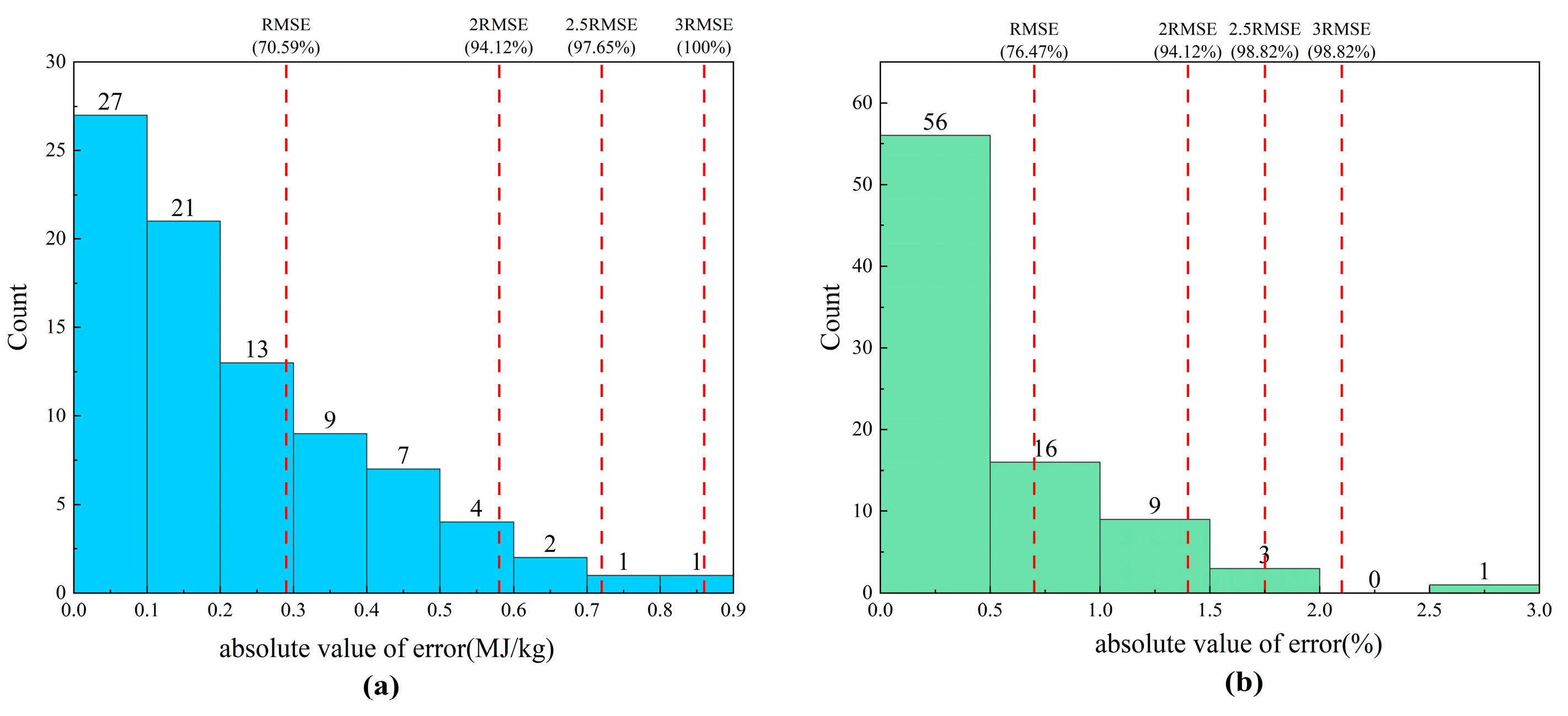
The calculation results demonstrate that among the 85 calibration samples (as presented in Table 5 and Figure 2), there are 60 samples (70.59%) where the absolute errors between the model-calculated low calorific value and the measured value are less than, or equal to, the RMSE of 0.29 MJ/kg. Additionally, there are 80 samples (94.12%) with errors within 2RMSE (0.58 MJ/kg); 83 samples (97.65%) with errors within 2.5RMSE (0.72 MJ/kg); and all 85 samples (100%) have errors within 3RMSE (0.86 MJ/kg).

3.2.2. C

Similarly, among the 85 calibration samples (as depicted in Figure 2), there are 65 samples (76.47%) with absolute errors of the model-calculated carbon content and the measured value ≤RMSE (0.70%); 80 samples (94.12%) with errors ≤2RMSE (1.40%); and 84 samples (98.82%) with errors ≤2.5RMSE (1.75%) and ≤3RMSE (2.10%).
In conclusion, the verifier can independently select thresholds within the range of 2RMSE to 3RMSE to judge the acceptability of low calorific value and carbon content data. Any data exceeding this threshold of absolute errors will be considered abnormal.

3.3. Validation of Regression Model

To validate the accuracy of the established models, 10 sets of data from the validation dataset were used. The results are presented in Table 6. In this study, 2.5RMSE is selected as the error threshold.
For the low calorific value, the absolute errors between the predicted values and the measured values of the 10 validation coal samples are within the error threshold of the regression model (2.5RMSE = 0.72 MJ/kg). The overall RMSE, MAE, and MRE for the validation dataset are 0.32 MJ/kg, 0.24 MJ/kg, and 1.27%, respectively.
Regarding the carbon content, the absolute errors between the calculated values and the measured values of the 10 coal samples are within the error threshold of the regression model (2.5RMSE = 1.75%). The overall RMSE, MAE, and MRE for the validation dataset are 0.80%, 0.68%, and 1.38%, respectively.
The results indicate that the established regression models for low calorific value and carbon content have a good fit and, to some extent, can effectively predict LCV and C.

4. Discussion

In order to examine the performance of the established models in screening, a comparison was made with the results obtained from existing empirical formulas, using the aforementioned validation dataset of 10 coal samples.

4.1. Comparison of the LCV Regression Models

Four typical regression models for the calorific value of coal, noted in references [6,7,8,9], were selected to be compared with the LCV model proposed in this study. This study focused on coal for the carbon market, resulting in a narrower coal sample range compared to others. Additionally, it is worth noting that these models express the predictions in different types of calorific values and on various bases, unlike the present model, which utilizes LCV on a received basis. For instance, the model by Chen et al. [6] presents the calorific values as LCV on an air-dried basis, while those by Kucukbayrak et al. [7] and Parikh et al. [8] express them as GCV on a dried basis. On the other hand, the model by Majumder et al. [9] provides the results in GCV on a received basis. To ensure consistency, the results reported in GCV on a dried basis and a received basis were adjusted to GCV on an air-dried basis according to the Chinese national standard (GB/T 35985-2018) [37]. Subsequently, a further conversion to LCV on a received basis was performed using the equation provided below:
L C V a r = ( G C V a d 206 H a d ) × 100 M t 100 M a d 23 M t
where Had is the hydrogen content of the coal on an air-dried basis in %, Mt is the total moisture content of the coal on a received basis in %, and Mad is the moisture content of the coal on an air-dried basis in %.
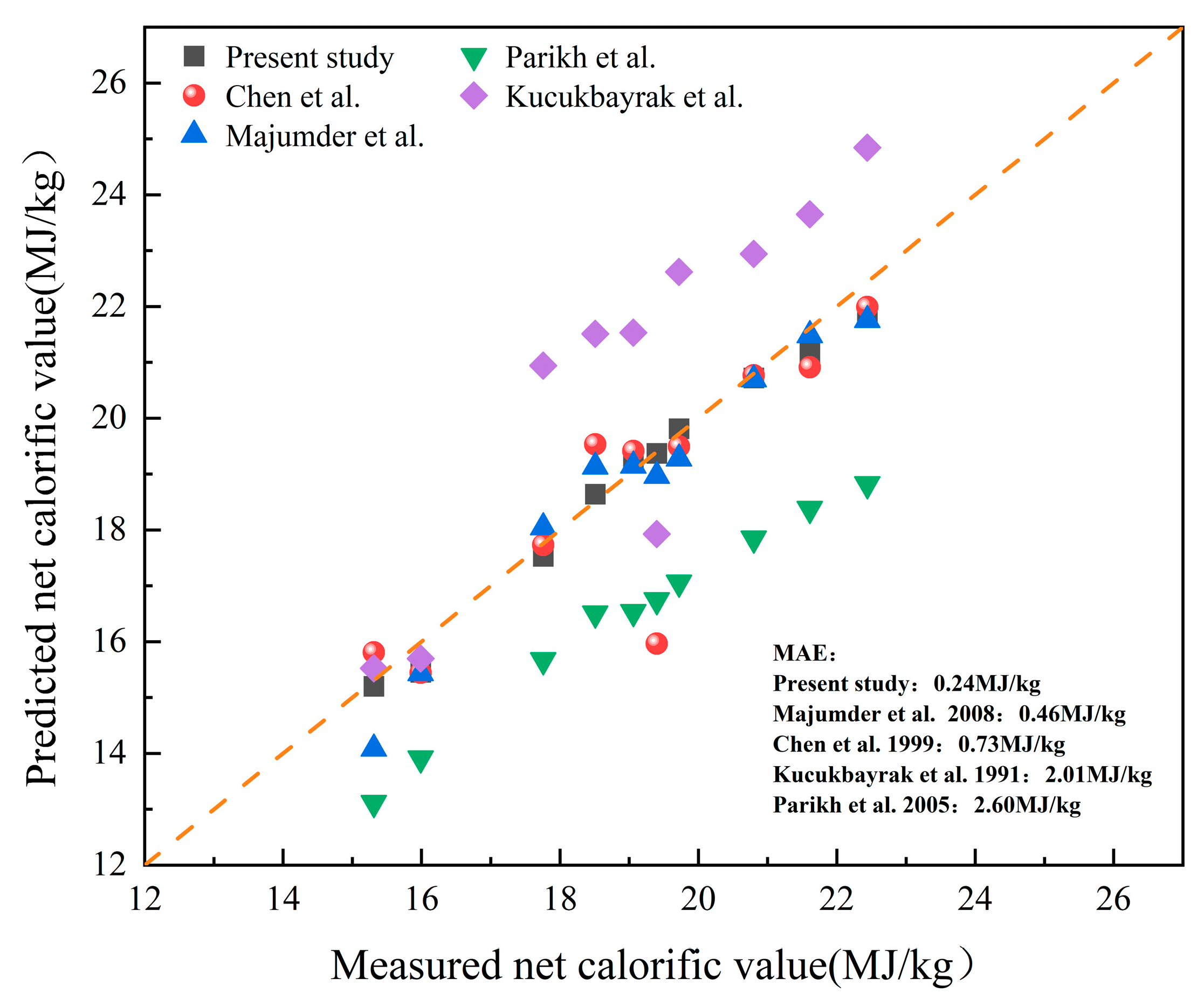
The comparison between the present model and the reference models in predicting the validation set is depicted in Figure 3. The present model demonstrates the lowest MAE of 0.24 MJ/kg, which is 2~10 times lower than that of the reference models. This suggests that the present model exhibits a significantly better fit to the validation of coal samples. Setting the threshold at 2.5RMSE = 0.72 MJ/kg, all ten sample data points fall within the acceptable region.
In contrast, the use of the reference models may not be effective as a screening method. Employing the same threshold of 0.72 MJ/kg, the models proposed by Chen et al. [6] and Majumder et al. [9] report 2 and 1 data points, respectively, out of the 10 data points falling outside the acceptable region. This observation aligns with the slightly larger MAEs reported by these models. Furthermore, the predictions made by Kucukbayrak et al. and Parikh et al. exhibit a relatively large discrepancy, with most data points falling outside the acceptable region; this may be attributed to the diverse fuel sample types and wider range of coal samples used for their model establishment, or possibly the parameter basis conversions.
In conclusion, the proposed LCV model in this study demonstrated a high level of suitability for effectively screening coal emission data, surpassing the performance of reference models.

4.2. Comparison of Carbon Content Regression Models

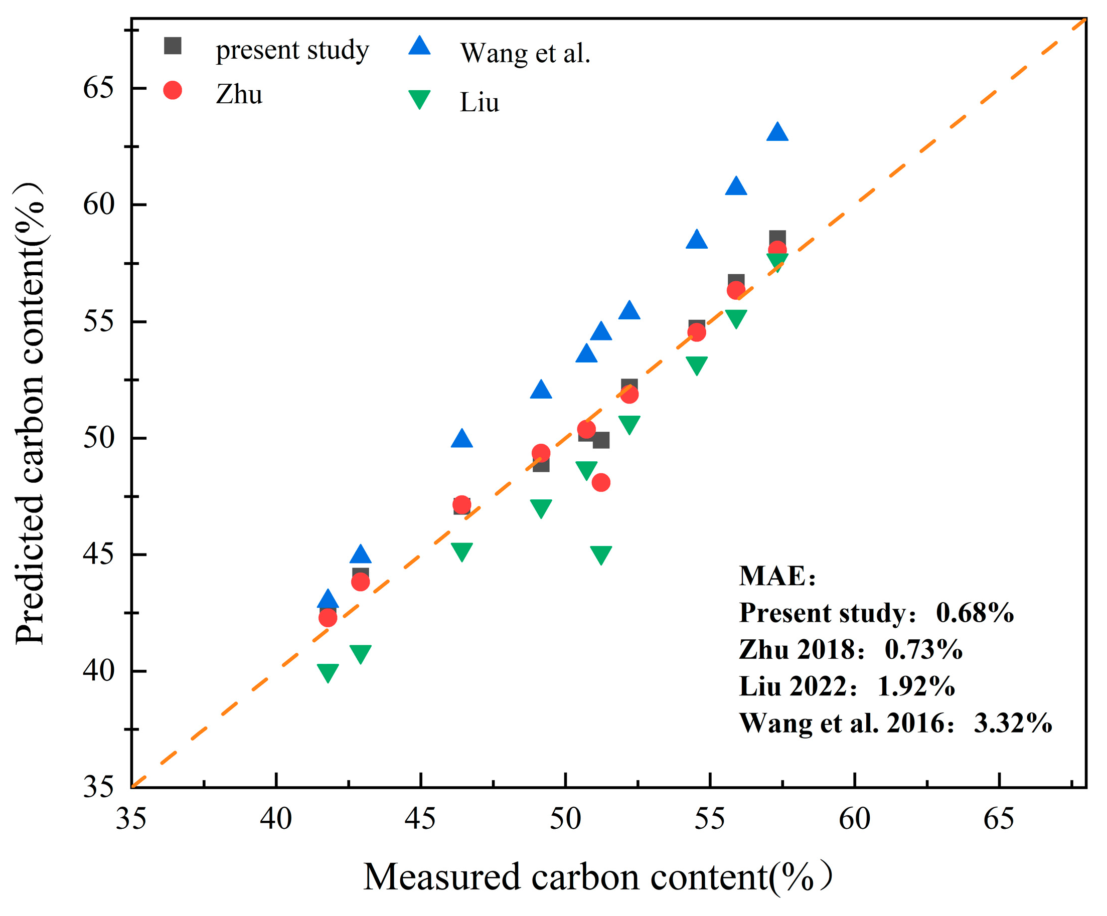
As the LCV and C of coal are mostly studied separately, three other typical regression models for estimating the carbon content of coal were chosen for comparison with the model developed in this study: models by Liu [26], Zhu [27], and Wang et al. [28]. To ensure a consistent basis for comparison, the reference models expressed at a different basis were converted to a received basis, in line with the present model. The outcomes of the carbon content regression model comparisons are illustrated in Figure 4.
The present model and the model proposed by Zhu exhibit the lowest MAE values for the validation samples—0.68% and 0.73%, respectively. One possible reason for such an agreement may be that the data sources used by both models were from coal-burning power plants. Additionally, the parameters used in both models, including LCV, V, and A, are quite similar, except for an additional parameter of S involved in Zhu’s model. When the acceptance threshold is set at 1.75%, all 10 data points are within the acceptance region according to both models.
However, the models of Liu and Wang et al. show higher MAEs of 1.92% and 3.32%, respectively. These models identified 5 and 9 questionable data points, respectively, out of the 10 validation samples. Notably, Wang’s model utilizes only one LCV parameter, to predict the carbon content. The significant discrepancy observed in their model highlights the criticality of careful parameter selection during model establishment. Additionally, the noticeable discrepancy in the model of Liu could be attributed to the utilization of different types of coal samples compared to the ones used in our study.
Overall, when compared with the reference models, the carbon content model proposed in the present study exhibits a higher level of suitability for screening the quality of coal data in the carbon market.

5. Conclusions

In this work, a fast screening method for the LCV and C of coal, based on MLR models used to assess the quality of coal data in the carbon market, was proposed. By employing MLR combined with the stepwise backward regression method, non-significant variables were gradually eliminated, resulting in highly accurate regression models for LCV and C. The major variables in the LCV regression model were identified as Mad, Stad, and Car, resulting in an R2 value of 0.9784, and RMSE, MAE, and MRE values of 0.32 MJ/kg, 0.24 MJ/kg, and 1.27%, respectively. The major variables in the C regression model were identified as Aad, Vad, and LCVar, with an R2 value of 0.9762, and RMSE, MAE, and MRE values of 0.80%, 0.68%, and 1.38%, respectively. The results of the LCV and C models demonstrated strong predictive capabilities. Additionally, this study determined that the optional error threshold interval of the LCV and C of coal is 2RMSE–3RMSE, which can serve as a reasonable judgment basis for carbon emission data during the verification process. The LCV and C models proposed in the present study exhibit a higher level of suitability for screening the quality of coal data in the carbon market in comparison with the reference models.
The screening method proposed in this study can serve as a valuable tool for verification agencies in evaluating the quality and reliability of carbon emission data in various regions, which can contribute to the promotion of standardized and orderly operation, as well as the sustainable development of the carbon emission trading market.

Author Contributions

Conceptualization and methodology, W.L.; software, X.C.; validation and formal analysis, X.C. and Z.S.; resources, Y.L.; project administration, J.L. All authors have read and agreed to the published version of the manuscript.

Funding

The study was supported by the National Key R&D Program of the Intergovernmental International Science and Technology Innovation Cooperation Project (2019YFE0109700); the Natural Science Foundation of Guangdong Province‘s Outstanding Youth Project (2021B1515020071); and the National Natural Science Foundation of China (U22B20119).

Data Availability Statement

Data are contained within the article.

Conflicts of Interest

The authors declare no conflict of interest.

References

  1. Chen, R.; Bao, Y.; Lv, F.; Chen, F.; Hu, K.; Zhang, Y. Coal measure energy production and the reservoir space utilization in China under carbon neutral target. Front. Earth Sci. 2023, 11, 1122040. [Google Scholar]
  2. Liu, W.; Xu, X.; Han, J.; Wang, B.; Li, Z.; Yan, Y. Trend model and key technologies of coal mine methane emission reduction reduction arming for the carbon neutrality. J. China Coal Soc. 2022, 47, 470–479. (In Chinese) [Google Scholar]
  3. Wang, W.; Kuang, Y.; Huang, N. Study on the Decomposition of Factors Affecting Energy-Related Carbon Emissions in Guangdong Province, China. Energies 2011, 4, 2249–2272. [Google Scholar] [CrossRef]
  4. Lu, W.; Chen, X.; Lu, J.; Li, Y.; Yao, S. Analysis and suggestion on carbon accounting of thermal power enterprises under the background of carbon peak and carbon neutrality. Clean Coal Technol. 2023, 10, 194–203. (In Chinese) [Google Scholar]
  5. Liu, Y.; Wang, D.; Ren, X. Rapid Quantitation of Coal Proximate Analysis by Using Laser-Induced Breakdown Spectroscopy. Energies 2022, 15, 2728. [Google Scholar] [CrossRef]
  6. Ren, Z.; Fang, C.; Zhao, J. Calorific value estimation of fire coal based on historical test data of incoming coal. Coal Qual. Technol. 2016, 18–20. (In Chinese) [Google Scholar]
  7. Kucukbayrak, S.; Durus, B.; Mericboyu, A.E.; Kadioglu, E. Estimation of calorific values of Turkish lignites. Fuel 1991, 70, 979–981. [Google Scholar] [CrossRef]
  8. Parikh, J.; Channiwala, S.A.; Ghosal, G.K. A correlation for calculating HHV from proximate analysis of solid fuels. Fuel 2005, 84, 487–494. [Google Scholar] [CrossRef]
  9. Majumder, A.K.; Jain, R.; Banerjee, P.; Barnwal, J.P. Development of a new proximate analysis based correlation to predict calorific value of coal. Fuel 2008, 87, 3077–3081. [Google Scholar]
  10. Akkaya, A.V. Proximate analysis based multiple regression models for higher heating value estimation of low rank coals. Fuel. Process. Technol. 2009, 90, 165–170. [Google Scholar] [CrossRef]
  11. Mesroghli, S.; Jorjani, E.; Chelgani, S.C. Estimation of gross calorific value based on coal analysis using regression and artificial neural networks. Int. J. Coal Geol. 2009, 79, 49–54. [Google Scholar] [CrossRef]
  12. Kavsek, D.; Bednarova, A.; Biro, M.; Kranvogl, R.; Voncina, D.B.; Beinrohr, E. Characterization of Slovenian coal and estimation of coal heating value based on proximate analysis using regression and artificial neural networks. Cent. Eur. J. Chem. 2013, 11, 1481–1491. [Google Scholar]
  13. Chelgani, S.C.; Makaremi, S. Explaining the relationship between common coal analyses and Afghan coal parameters using statistical modeling methods. Fuel. Process. Technol. 2013, 110, 79–85. [Google Scholar] [CrossRef]
  14. Given, P.H.; Weldon, D.; Zoeller, J.H. Calculation of calorific values of coals from ultimate analyses: Theoretical basis and geochemical implications. Fuel 1986, 65, 849–854. [Google Scholar] [CrossRef]
  15. Channiwala, S.A.; Parikh, P.P. A unified correlation for estimating HHV of solid, liquid and gaseous fuels. Fuel 2002, 81, 1051–1063. [Google Scholar] [CrossRef]
  16. Feng, Q.; Zhang, J.; Zhang, X.; Wen, S. Proximate analysis based prediction of gross calorific value of coals: A comparison of support vector machine, alternating conditional expectation and artificial neural network. Fuel Process. Technol. 2015, 10, 120–129. [Google Scholar] [CrossRef]
  17. Erik, N.Y.; Yilmaz, I. On the Use of Conventional and Soft Computing Models for Prediction of Gross Calorific Value (GCV) of Coal. Int. J. Coal Prep. Util. 2011, 31, 32–59. [Google Scholar] [CrossRef]
  18. Wen, X.; Jian, S.; Wang, J. Prediction models of calorific value of coal based on wavelet neural networks. Fuel 2017, 199, 512–522. [Google Scholar] [CrossRef]
  19. Patel, S.U.; Kumar, B.J.; Badhe, Y.P.; Sharma, B.K.; Saha, S.; Biswas, S.; Chaudhury, A.; Tambe, S.S.; Kulkarni, B.D. Estimation of gross calorific value of coals using artificial neural networks. Fuel 2007, 86, 334–344. [Google Scholar] [CrossRef]
  20. Chelgani, S.C.; Hart, B.; Grady, W.C.; Hower, J.C. Study relationship between inorganic and organic coal analysis with gross calorific value by multiple regression and ANFIS. Int. J. Coal Prep. Util. 2011, 31, 9–19. [Google Scholar] [CrossRef]
  21. Qi, M.; Luo, H.; Wei, P.; Fu, Z. Estimation of low calorific value of blended coals based on support vector regression and sensitivity analysis in coal-fired power plants. Fuel 2019, 236, 1400–1407. [Google Scholar]
  22. Tan, P.; Zhang, C.; Xia, J.; Fang, Q.; Chen, G. Estimation of higher heating value of coal based on proximate analysis using support vector regression. Fuel Process. Technol. 2015, 138, 298–304. [Google Scholar] [CrossRef]
  23. Matin, S.S.; Chelgani, S.C. Estimation of coal gross calorific value based on various analyses by random forest method. Fuel 2016, 177, 274–278. [Google Scholar]
  24. Saptoro, A.; Vuthaluru, H.B.; Tade, M.O. A comparative study of prediction of elemental composition of coal using empirical modelling. IFAC Proc. Vol. 2006, 39, 747–752. [Google Scholar]
  25. Yi, L.; Feng, J.; Qin, Y.; Li, W. Prediction of elemental composition of coal using proximate analysis. Fuel 2017, 193, 315–321. [Google Scholar] [CrossRef]
  26. Liu, F. A comparison between multivariate linear model and maximum likelihood estimation for the prediction of elemental composition of coal using proximate analysis. Results Eng. 2022, 13, 100338. [Google Scholar]
  27. Zhu, D. Application of Carbon Ultimate Analysis into Greenhouse Gas Emissions Accounting for Coal-fired Power Plants. Power Gener. Technol. 2018, 39, 363–366. (In Chinese) [Google Scholar]
  28. Wang, Y.; Huang, J.; Wang, Y. Discussion on Deriving Formula of Carbon Content and CO2 Emissions from Coal Calorific. Northeast Electr. Power Technol. 2016, 37, 5–7. (In Chinese) [Google Scholar]
  29. Wen, X.; Li, G.; Sun, L.; Sun, Y.; Wang, G. Analysis of Carbon in Coal-fired Based on Partial Least Squares Regression Algorithm. J. Northeast Dianli Univ. 2012, 32, 31–36. (In Chinese) [Google Scholar]
  30. Wen, X.; Sun, L. Analysis on Coal-fired Carbon Based on Support Vector Machine. East China Electr. Power 2011, 39, 973–976. (In Chinese) [Google Scholar]
  31. Xu, Q.; Wang, Y.; Lin, W.; Liang, H.; Wan, J. Calculation of CO2 emissions in boilers based on ACO-LSSVM method for carbon element analysis of coal. J. Fuzhou Univ. Nat. Sci. Ed. 2015, 43, 548–553. (In Chinese) [Google Scholar]
  32. Bienvenido-Huertas, D.; Rubio-Bellido, C.; Perez-Ordoez, J.L.; Martínez-Abella, F. Estimating Adaptive Setpoint Temperatures Using Weather Stations. Energies 2019, 12, 1197. [Google Scholar]
  33. Ghani, I.M.M.; Ahmad, S. Stepwise Multiple Regression Method to Forecast Fish Landing. Procedia-Soc. Behav. Sci. 2010, 8, 549–554. [Google Scholar] [CrossRef]
  34. Lu, Z.; Chen, X.; Yao, S.; Qin, H.; Zhang, L.; Yao, X.; Yu, Z.; Lu, J. Feasibility study of gross calorific value, carbon content, volatile matter content and ash content of solid biomass fuel using laser-induced breakdown spectroscopy. Fuel 2019, 258, 116150. [Google Scholar]
  35. Chang, H.; Sun, W.; Gu, X. Forecasting Energy CO2 Emissions Using a Quantum Harmony Search Algorithm-Based DMSFE Combination Model. Energies 2013, 6, 1456–1477. [Google Scholar] [CrossRef]
  36. Szer, M.; Haykiri-Acma, H.; Yaman, S. Prediction of Calorific Value of Coal by Multi Linear Regression and Analysis of Variance. J. Energ. Resour-ASME 2021, 144, 1–28. [Google Scholar]
  37. GB/T 35985-2018; Calculation of Analyses to Different Bases for Coal. Standards Press of China: Beijing, China, 2018.
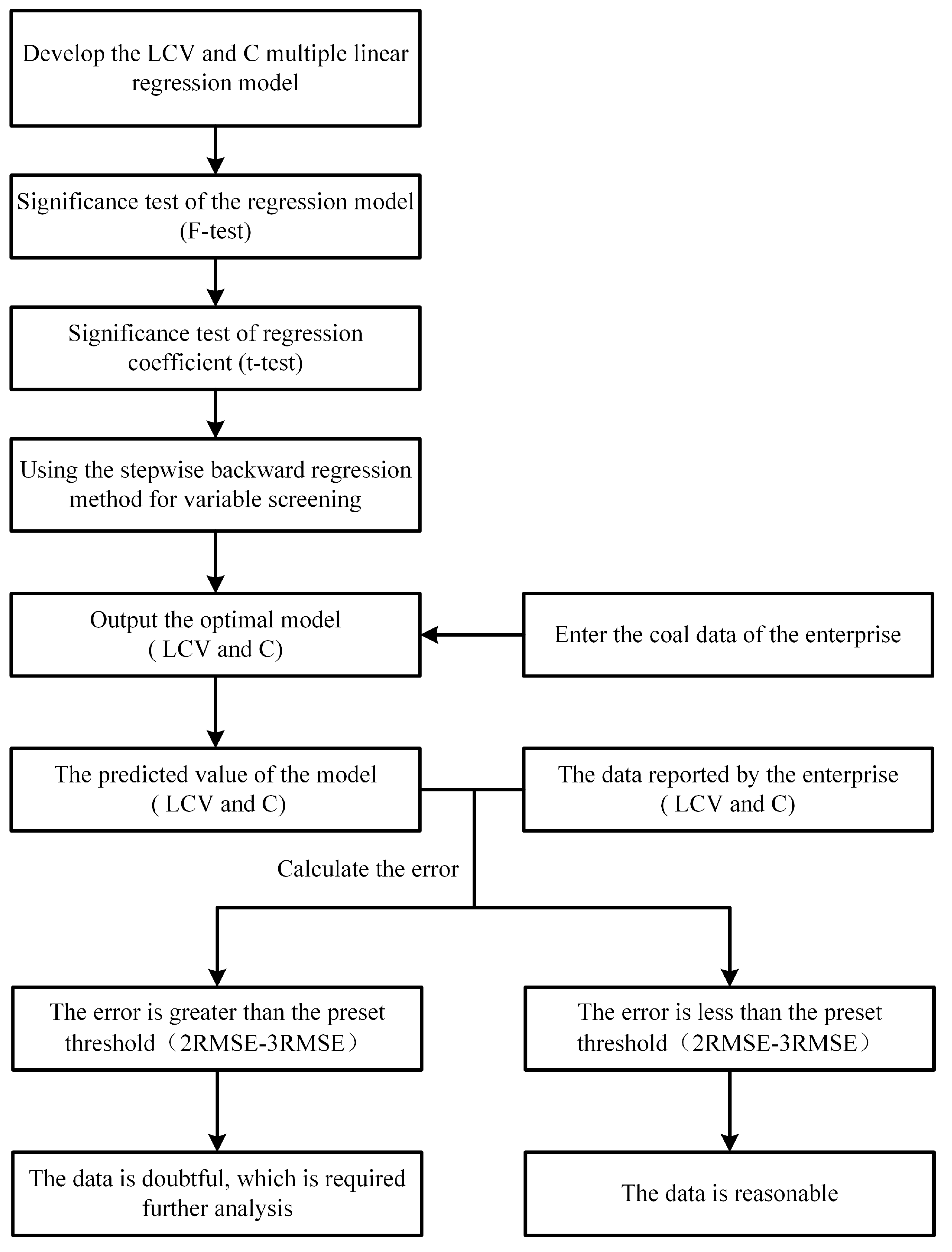
Figure 1. The flow chart of the methodology of this study.
Energies 16 07592 g001
Figure 2. Distribution of absolute errors: (a) low calorific value; (b) carbon content.
Energies 16 07592 g002
Figure 3. Comparison between the predicted value and the measured data for the net calorific value of coal [6,7,8,9].
Energies 16 07592 g003
Figure 4. Comparison between the predicted value and the measured data for the carbon content of coal [26,27,28].
Energies 16 07592 g004
Table 1. Survey of published correlations the between calorific value and carbon content of coal.
ParameterReferenceModelModel Evaluation Indicators
Calorific valueChen et al. (1999) [6]LCV = 35,860 − 73.7V − 395.7A − 702Mn.g.
Kucukbayrak et al. (1991) [7]GCV = 76.56 − 1.30(V + A) + 7.03 × 10⁻³(V + A)2R2 = 0.91
Parikh et al. (2005) [8]GCV = 0.3536FC + 0.1559V − 0.0078AMAE = 3.74%
Majumder et al. (2008) [9]GCV = −0.03A − 0.11M + 0.33V + 0.35FCMAE = 1.49%
Akkaya (2009) [10]GCV = 0.836M−8.155A−3.559V0.35FC0.626
GCV = 0.561M−6.137V0.381FC0.666
GCV = 33.078 − 0.72M + 0.012M2 − 1.163M3 − 0.324A2
R2 = 0.97
Mesroghli et al. (2009) [11]GCV = 37.777 − 0.647M − 0.387A − 0.089V
GCV = −26.29 + 0.275A + 0.605C + 1.352H + 0.840N + 0.321S
R2 = 0.97
Kavsek et al. (2013) [12]GCV = −3.57 + 0.31V + 0.34FCR2 = 0.971
Chelgani et al. (2013) [13]GCV = 35.391 − 0.47M − 0.364A − 0.028V
GCV = −0.408 + 1.243H + 0.348C−0.1N − 0.111O + 0.112S
R2 = 0.998
Given et al. (1986) [14]GCV = 0.3278C +1.419H + 0.09257S − 0.1379O + 0.637n.g.
Channiwala et al. (2002) [15]GCV = 0.3491C + 1.1783H + 0.1005S − 0.1034O − 0.0151N − 0.0211AMAE = 1.45%
Carbon contentSaptoro et al. (2006) [24]C = a0 + a1A + a2V + a3M + a4FCn.g.
Yi et al. (2017) [25]C = x1 + x2A + x3A2 + x4V + x5V2 + x6FC + x7FC2
(1) Anthracite:
C = 306,540 − 3066.61A + 0.0229439A2 − 3066.31V + 0.0435868V2 − 3063.36FC − 0.0106054FC2
(2) High-rank bituminous:
C = −143,398 + 1434.61A − 0.0138486A2 + 1435.78V − 0.0125349V2 + 1433.88FC + 0.0106647FC2
(3) Subbituminous:
C = 40,521.2 − 403.482A − 0.085603A2 − 403.029V − 0.0193969V2 − 405.885FC + 0.0168029FC2
(4) Lignite:
C = 5855.8 − 57.3735A − 0.0220361A2 − 58.4226V + 0.0131499V2 − 58.9345FC + 0.0195368FC2
(1) Anthracite:
R2 = 0.95, MAE = 0.53%
(2) High-rank bituminous:
R2 = 0.93, MAE = 0.51%
(3) Subbituminous:
R2 = 0.86, MAE = 0.93%
(4) Lignite:
R2 = 0.92, MAE = 1.87%
Liu (2022) [26]C = 50.7368 − 0.5799FC − 0.7066V + 2.8301GCVMAE = 1.97%
Zhu (2018) [27]C = 35.411 − 0.341A − 0.199V − 0.412S + 1.632GCVn.g.
Wang et al. (2016) [28](1) C = LCV/356 (LCV: 5026–19,040 kJ/kg)
(2) C = LCV/383 (LCV: 19,040–29,850 kJ/kg)
RE = −0.6~1.14%
Note: C, H, O, N, S, M, A, V, FC, GCV, and LCV represent contents of carbon, hydrogen, oxygen, nitrogen, sulphur, moisture, ash, volatile matter, fixed carbon, gross calorific value, and lower calorific value, respectively; n.g. represents not given.
Table 2. Descriptive statistics of coal sample data.
Coal PropertyMinimumMaximumMeanStandard Deviation
Mad (%)2.4819.927.244.04
Aad (%)3.6934.0618.486.91
Vad (%)25.5242.4131.144.57
FCad (%)34.0760.7443.384.04
St,ad (%)0.121.980.770.31
Had (%)3.234.413.710.24
Car (%)39.9061.1450.724.69
LCVar (MJ/kg)14.8522.7819.052.02
Note: Mad: moisture content on an air-dried basis; Aad: ash content on an air-dried basis; Vad: volatile matter content on an air-dried basis; FCad: fixed carbon content on an air-dried basis; Had: hydrogen content on an air-dried basis; Car: carbon content on an as-received basis; LCVar: lower calorific value content on an as-received basis.
Table 3. Variance results for the low calorific value model.
ModelCoefficientSig.(t)Sig.(F)R2
1Intercept−2.1160.4463.53 × 10−620.9775
Mad−0.0250.384
St,ad0.3940.033
Car0.3934.91 × 10−41
Had0.1510.565
FCad0.010.647
Aad0.0040.882
Vad0.000320.993
2Intercept−2.0970.21.36 × 10−630.9778
Mad−0.0250.325
St,ad0.3950.027
Car0.3932.21 × 10−47
Had0.1520.504
FCad0.010.564
Aad0.0040.797
3Intercept−1.7260.0244.85 × 10−650.9781
Mad−0.030.06
St,ad0.4080.017
Car0.3935.64 × 10−48
Had0.1070.454
FCad0.0080.601
4Intercept−1.6040.0271.69 × 10−660.9783
Mad−0.0340.016
St,ad0.3710.016
Car0.3979.91 × 10−59
Had0.120.392
5Intercept−1.2020.0276.32 × 10−680.9784
Mad−0.0320.021
St,ad0.3590.019
Car0.3981.77 × 10−59
Table 4. Variance results for the carbon content model.
ModelCoefficientSig.(t)Sig.(F)R2
1Intercept13.8190.0378.32 × 10−610.9756
Aad−0.0980.17
Vad−0.1410.126
Qnet,ar2.3014.91 × 10−41
St,ad−0.5330.238
FCad−0.0180.737
Mad0.0130.853
Had0.1080.866
2Intercept13.8810.0353.39 × 10−620.9759
Aad−0.0980.168
Vad−0.1340.095
Qnet,ar2.3058.81 × 10−43
St,ad−0.5290.238
FCad−0.0170.744
Mad0.0110.873
3Intercept14.7291.35 × 10−41.24 × 10−630.9762
Aad−0.1070.016
Vad−0.1420.023
Qnet,ar2.3016 × 10−45
St,ad−0.5330.231
FCad−0.0240.483
4Intercept13.5538 × 10−55.04 × 10−650.9764
Aad−0.0950.02
Vad−0.1260.029
Qnet,ar2.2733.48 × 10−50
St,ad−0.5490.215
5Intercept15.6493.07 × 10−72.96 × 10−660.9762
Aad−0.1293.40 × 10−5
Vad−0.1590.002
Qnet,ar2.2287.99 × 10−56
Table 5. Proportion of acceptable sample data within different error thresholds.
Absolute ErrorsProportion of Model Calculated Value (%)
Low Calorific Value
(RMSE = 0.29 MJ/kg)
Carbon Content
(RMSE = 0.70%)
≤RMSE70.5976.47
≤2RMSE94.1294.12
≤2.5RMSE97.6598.82
≤3RMSE10098.82
Table 6. Results of regression model validation.
SampleLCVarCar
Measured Value
(MJ/kg)
Predicted Value
(MJ/kg)
Absolute Error
(MJ/kg)
Relative Error
(%)
Measured Value
(%)
Predicted Value
(%)
Absolute Error
(%)
Relative Error
(%)
122.4421.82−0.622.7757.3358.551.222.12
221.6121.18−0.432.0055.9056.690.791.41
319.7219.810.090.4452.2152.20−0.010.01
419.4019.37−0.030.1351.2349.92−1.312.56
519.0619.230.170.9050.7350.22−0.511.00
617.7617.53−0.231.3146.4247.080.661.42
718.5118.640.130.7149.1648.91−0.250.50
820.8020.72−0.080.3954.5454.730.190.35
915.3115.20−0.110.6941.7942.500.711.70
1015.9915.45−0.543.4042.9244.081.152.69
Disclaimer/Publisher’s Note: The statements, opinions and data contained in all publications are solely those of the individual author(s) and contributor(s) and not of MDPI and/or the editor(s). MDPI and/or the editor(s) disclaim responsibility for any injury to people or property resulting from any ideas, methods, instructions or products referred to in the content.