1. Introduction
The phenomenon of percolation comes from chemistry in connection with the gelation of polymers during World War II [
1]. Percolation theory is used in the description of various systems and phenomena, including the spread of epidemics [
2], the reliability of computer networks [
3], the spread of fires [
4], molecular biology [
5,
6], materials science [
7] and the flow of electricity by conductive and non-conductive mixtures [
8]. Currently, the percolation phenomenon is widely used to describe DC and AC conductivity in metal–dielectric nanocomposites. This is the so-called hopping conductivity based on the quantum mechanical phenomenon of electron tunnelling [
9,
10,
11,
12]. Research on percolation has been growing rapidly since the 1950s. Currently, over 10,000 articles with the term “percolation” have been registered in the Web of Science Core Collection database. Moreover, there are many articles that have reported percolation studies without using the term in their titles. The phenomenon of percolation (Latin percolatio—a straining or filtering through) is a critical phenomenon. It describes the type 2 phase transitions due to the continuous change in parameters. It is an idea that is difficult to define precisely, although it is quite easy to describe qualitatively. The first article by Flory-Stockmayer [
13] on the percolation theory was published in 1952 [
14]. However, S. R. Broadbent and J. M. Hammersley [
15] are the pioneers of the theory of percolation phenomena. In physical terms, the definition of percolation is quite general. In a medium made up of at least two phases, the elements of one phase, called dispersed, which are independent, under certain conditions form a more complex structure that changes the macroscopic properties of the entire medium. This is a consequence of a change in the concentration of the dispersed phase. The percolation theory includes models of flat and spatial random processes and the effects of the variable range of their mutual interactions and is used to describe systems with stochastic geometry and topologically disordered bodies [
16]. This idea is illustrated by the network that was created by Broadbent and Hammersley as the first, simple, stochastic model [
15]. Such a network consists of
n-dimensions and can be both regular and irregular. It has a finite number of nodes, the distribution of which is determined by the type of the considered network and may be random or determined by the type of network. In such a model, nodes are assigned to two states, open or closed. The volume, number or concentration of open nodes is determined by
x. They are distributed randomly with the probability
p. For a small number of open nodes in relation to closed nodes, it is impossible to create the so-called percolation channel between two opposite planes of the network, i.e., a continuous connection of open nodes. This is due to the fact that the number of nodes making up the channel, even for the shortest straight line, is insufficient to connect the network planes. Both the nodes and the clusters they create as a result of aggregation are isolated. Then the percolation probability denoted by
P(
p) is 0. With an increase in the number of connections, density, filling or concentration in disordered systems, the percolation threshold suddenly occurs. There is a value of
x for which the probability of percolation is non-zero since the number of nodes making up the percolation channel is sufficient to create a continuous connection. This value is denoted
xc and is called the percolation threshold. Further increasing the value of
x causes the formation of larger clusters, expansion of the resulting channel or the creation of new ones. The appearance of the percolation threshold determines the creation of a so-called infinite percolation cluster. Such a cluster takes an irregular geometric shape. Percolation phenomena can be divided into two main groups based on the types of connections, i.e., bond percolation and site percolation [
17,
18]. In bond percolation, open and closed states are assigned to connections between nodes, while in site percolation, these states are assigned to nodes. Both are models belonging to discrete percolation. This term is used to describe percolation theory models in which the media are discrete sets, such as sets of regular lattice points, or more generalised examples such as graphs. In addition to the site and bond percolation models, there are others that are a variation of these two types. An example is the percolation of two-phase continuous systems (Swiss cheese model) called continuous percolation. This model differs from site percolation in that the objects that make up the nodes are of any shape and size. In the case of three-dimensional networks, they can be cubes, canes or spheres, and in two-dimensional models, there are circles, ellipses, segments, etc. These objects are randomly placed in a non-conductive environment and are part of the system forming a percolation channel [
19,
20]. There is also a model of stirred percolation [
21], polychromatic percolation [
22] or bootstrap percolation [
23]. The phenomenon of percolation is also analysed in terms of two main types of networks: random networks and those with translational symmetry. Over the past few decades, an enormous amount of work has been completed to find the exact and approximate percolation thresholds for different networks. The exact thresholds are known only for some two-dimensional networks. Examples are square networks (4
4), in which the threshold for bond percolation is exactly 0.5, or triangular networks (3
6), where the site percolation threshold is also 0.5 These values have been proven analytically [
24]. It was possible because these networks can be divided into a self-similar pattern, i.e., after a triangle–triangle transformation, the system remains the same. Two-dimensional self-modality means that all fully triangulated networks (e.g., triangle, union jack, double cross, double martini and double asanoha, or double 3–12 and Delaunay triangulation) have a site percolation threshold of 0.5. In other cases, it is not possible, which resulted in the construction of models.
The model that describes the behaviour of fluids in porous media was the most primary and developed at the earliest [
25]. It was presented as an analogy network of capillary tubes, which reflected the geometry of the rock sample, thanks to which parameters such as permeability, capillary pressure, capillary growth rate and saturation level were estimated. This model, even though it was based on the percolation theory, provided a lot of information about capillary flow without contributing much to the study of the percolation phenomenon. To model the percolation phenomenon in order to determine the percolation threshold, the most obvious one was the flow of electric current in a two-dimensional model of a square network composed of conductive and insulating elements [
26]. Electric current will begin to flow between the electrodes at opposite edges of the matrix when the contacting conductive spheres create a conductive channel called a percolation channel, i.e., a continuous connection between the electrodes.
It is intuitively known that there is a critical value of the conductive sphere concentration for which such a channel will be created. For a small number of spheres
n <
L it is impossible to create a percolation channel between two electrodes. This is because the number of spheres forming the channel is insufficient even for the shortest straight line connecting the opposite sides of the network. Both the nodes and the clusters they create, i.e., groups of adjacent conductive nodes formed as a result of aggregation, are isolated. When analysing a square matrix with dimensions
L·
L, the minimum number of conducting spheres to reach the percolation threshold is
L. However, there is a very small probability of a random distribution of spheres, which will result in a system that connects two opposite edges of the matrix in a straight line. There is also a number of conductive spheres for which the percolation probability
P(
p) = 1. For a given network example, this number is (
L2 −
L + 1). This means that the percolation threshold is in the sphere concentration range
L ≤
xc ≤ (
L2 −
L + 1). Thus, it cannot be determined based on a single iteration only. This problem needs to be identified and solved statistically. In order to achieve statistics with a high confidence coefficient, a given type of network should be repeatedly modelled. In the pre-computer era, this was technically very difficult to do. With the advent of the computer age, when the limitations of computational tools ceased to be a barrier, the phenomenon of percolation began to be analysed using the Monte Carlo method. The possibility of using the Monte Carlo method in the study of percolation resulted in the creation of numerous models. The most frequently studied models were two-dimensional networks with translational symmetry. Such a network was transformed into a random one by occupying points (vertices) or bonds (edges) with a statistically independent probability
p. Depending on the method of the network obtaining, models of bond percolation or knot percolation, respectively, were created. These models assume that the occupied places or bonds are completely random (Bernoulli percolation). The percolation thresholds for many networks were estimated, incl. honeycombs (6
6) [
27,
28], Kagome (6, 3, 6, 3) [
29,
30], rhombitrihexagonal (3, 4, 6, 4) [
31], maple leaf (3
4, 6) [
31,
32], non-planar chimera [
33], subnetworks [
34], many other three-dimensional [
26] and even for dimensions larger than 3 [
35]. One of the first statistical calculations of the node percolation threshold for a square matrix appeared in the 1960s with a result of 0.569(13)% [
36]. The simulations were made for a square matrix with dimensions
L = 78, and number of iterations
n = 30. From the nineties of the last century until now, the intensification of research and increase in computational possibilities have provided more accurate results of the calculations. The publications give the values 0.59274605079210(2) [
30], 0.59274601(2) [
28], 0.59274621(13) [
37], 0.59274621(33) [
38]. The simulation results in the above works differ by no more than one ten-thousandth of a percent. In the publication [
37] for the calculation of the site percolation threshold using the Monte Carlo method, a statistical calculation algorithm was assumed, which provides the result with a very large number of iterations and a much lower demand for computing power. The calculations were performed for the matrix with the size
L = 256 for a very large number of iterations, amounting to 3 × 10
8. The estimation result was
pc = 0.59274621(13).
Unfortunately, most of the publications quoted above do not provide such model parameters as the dimensions of matrixes used in the simulations and the number of iterations. Moreover, the recommendations of the document [
39], concerning the metrological analysis of the measurement results, which are undoubtedly the values of the percolation threshold and the uncertainty of their estimation, were not applied. According to this document and its earlier versions, to estimate the numerical values based on random variables, obtained with repeated repetition of measurements using statistical methods, the measurement uncertainty of type A is used [
39]. This means that at first it should be specified if the obtained sequence of results corresponds to a normal distribution. According to this document, the full (correct) measurement in this case consists of the measured value and the measurement uncertainty. The measured value in the case of multiple repetitions of the measurement is equal to the arithmetic mean value of the subsequent measurement results. The measurement uncertainty is a function of the standard deviation and the number of iterations. In the work, the metrological approach for estimating the measurement uncertainty was used to analyse the results of the Monte Carlo simulation of the percolation phenomenon for many iterations. Such an analysis, together with other model parameters, such as the use of different dimension matrixes and the variation of the number of iterations, allows us to obtain new data on the percolation phenomenon in the so far analysed square matrixes.
The aim of the work is:
Simulation of the site percolation phenomenon using the Monte Carlo method with the use of inverted simulation logic for square matrixes with dimensions L = 55, 101 and 151 for a large number of iterations 5 × 10⁶;
Determination of the node’s initial coordinates and their distribution in space, generated in each iteration, and on their basis confirmation of the software generating non-conductive nodes in the matrixes correct operation;
Determination of the percolation threshold value for each iteration;
Determination of the probability statistical distribution of the percolation threshold value occurrence;
Determination of the average value of the percolation threshold, standard deviation and the uncertainty of the percolation threshold estimation dependence on the number of iterations;
The impact of the matrix dimensions on the values of the percolation threshold, standard deviation and the uncertainty of the percolation threshold estimation analysis.
2. Methods
Exact percolation thresholds, determined analytically, are known only for some two-dimensional networks. This is the square network, denoted as (44), for which the node percolation threshold is exactly 0.5, and the triangular network (36), where the node percolation threshold value is also 0.5 [
24]. In other types of networks, for example, the square network for node percolation and the triangular network for bond percolation, the percolation threshold can only be determined by computer simulation. Therefore, the object of the Monte Carlo simulation was the square network for node percolation.
The most common percolation model is to define a regular network, such as a quadratic one, and transform it into a random network by randomly “occupying” sites (vertices) or bonds (edges) with a statistically independent probability
p [
24,
40,
41]. When a critical probability value
pc is reached, the so-called long-range connectivity appears for the first time and a percolation channel is formed, allowing current to flow. The value of
pc is called the percolation threshold. The percolation of nodes in a two-dimensional square network is the most studied percolation model by simulation methods. It is a special type of network because the square network has the property of self-duality [
42].
The first step of the Monte Carlo computer simulation was to define the space in which the problem would be analysed. In this case, it is an L2 square matrix whose nodes are described in the Cartesian plane. Despite the simplification of the model to two dimensions, the simulation calculations are performed sequentially, so the choice of the L parameter determines the time of the performed simulation.
Next, the logic of the model under study was determined. According to percolation theory, in the simulation, all
K nodes of the quadratic network belong to the set
E:
A sequential permutation without repetition of K nodes on the set E was then performed, which were assigned to subsets of the set G such that:
If the set G = Ø, the node K forms a subset of the set G.
If node K was the nearest node in the vertical, horizontal or diagonal direction of a node from the set G, it was added to the subset containing that node.
If the node K was the nearest node in the vertical, horizontal or diagonal direction of more than one point from the set G and these points belong to different subsets of the set G then the subsets are replaced by their conjunction with the added point K.
Regarding percolation, all subsets in the set G are clusters composed of neighbouring nodes of the network.
The above conditions define the reverse direction of percolation, i.e., the determination of the concentration
N for which at least one subset will form a critical cluster [
43]. This will be the concentration for which the last percolation channel of the network is broken. This means that the initial state of the matrix is the state in which all nodes of the matrix are occupied by conducting elements. In the case of a square matrix, the conductive nodes are in contact with their neighbouring nodes, arranged in vertical and horizontal directions. This state of the matrix results in current flow when electrodes are connected to a current source, contacting the conductive elements of the matrix at its top and bottom edges. The next simulation steps involve randomly eliminating individual conductive elements and replacing them with non-conductive nodes. As the number of non-conductive elements increases, clusters appear, until finally the removal of a single conductive element, which results in the complete disconnection of the top electrode from the bottom electrode and the interruption of current flow. This means that the percolation threshold
xc is reached. Previous studies [
44] show that the expected percolation threshold for a two-dimensional square lattice is about 0.59. This means that the use of conduction element elimination is an optimisation action. In the case of adding conductive nodes, the number of nodes is about 0.59. In the case of elimination, about 0.41 nodes must be removed. This means that the algorithm to remove conductive elements requires approximately 1.44 times fewer calculations.
The algorithm and simulation software for this thesis was developed in the Python programming language in the Unix system environment. The calculations were based on multiplicity theory because the computer performs assignment processes much faster than computational processes. The only variable was the dimension of the square lattice L.
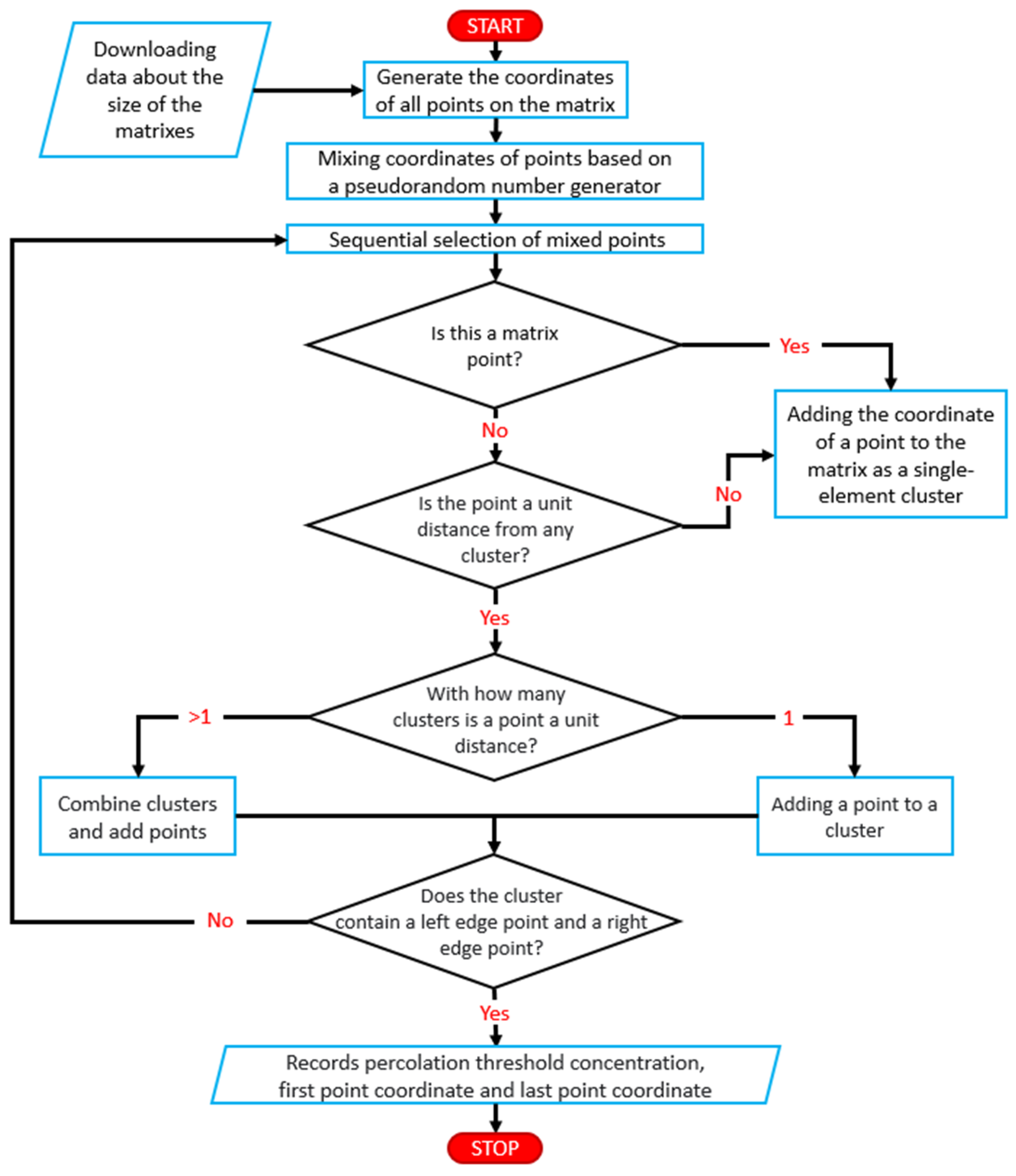
Figure 1 shows a schematic diagram of the computer software algorithm developed to simulate the percolation phenomenon using the Monte Carlo method. In the first step of the simulation, the computer created a set of square network nodes with coordinates of dimension
L·
L. Then, using a pseudo-random number generator, the set was randomly mixed. The pseudo-random number generator implemented for the simulation is based on a basic function that generates a random regular floating-point number in the semi-open range [0,1). The main generator is the “Mersenne Twister” algorithm [
45] which generates floating point numbers with a precision of 53 bits in the range 219937-1 and is a basic implementation in the C programming language. The MT19937 variant used has a high degree of uniform distribution which means that the periodic dependence between successive values of the output sequence is negligible. It also satisfies numerous statistical randomness tests, including diehard tests. It satisfies most, but not all, of the more rigorous randomness tests (e.g., TestU01 Crush) [
45]. The “Mersenne Twister” algorithm is used in many Monte Carlo studies [
46,
47,
48,
49].
The software then performed a sequential selection of a non-conductive nodes set. The first node drawn formed a one-element set. Each subsequent non-conductive node selected was subject to a membership check of the existing sets, i.e., if the selected node was within a unit distance in the vertical, horizontal or diagonal direction from any node in the existing set. It was then attached to this set to form a cluster. Otherwise, the node formed a one-element set. The exception was when the selected node belonged to more than one cluster. Then it was added to the combined clusters. Once a non-conducting node was added to an existing cluster, that cluster was tested to see if it contained points with coordinates x = 0 and x = L. This condition determined whether the cluster formed a continuous connection between the right and left edges of the matrix. Meeting these conditions means that a so-called “infinite cluster” is formed from non-conducting nodes and the percolation threshold is reached. The algorithm at this stage stored the coordinates of the first drawn node, the coordinates of the non-conducting node interrupting the last percolation channel and the calculated percolation threshold concentration and terminated its operation. The algorithm was run again until a preset number of iterations was obtained, which was 5 × 10⁶. Simulations were performed for matrixes of size L = 55, 101 and 151.
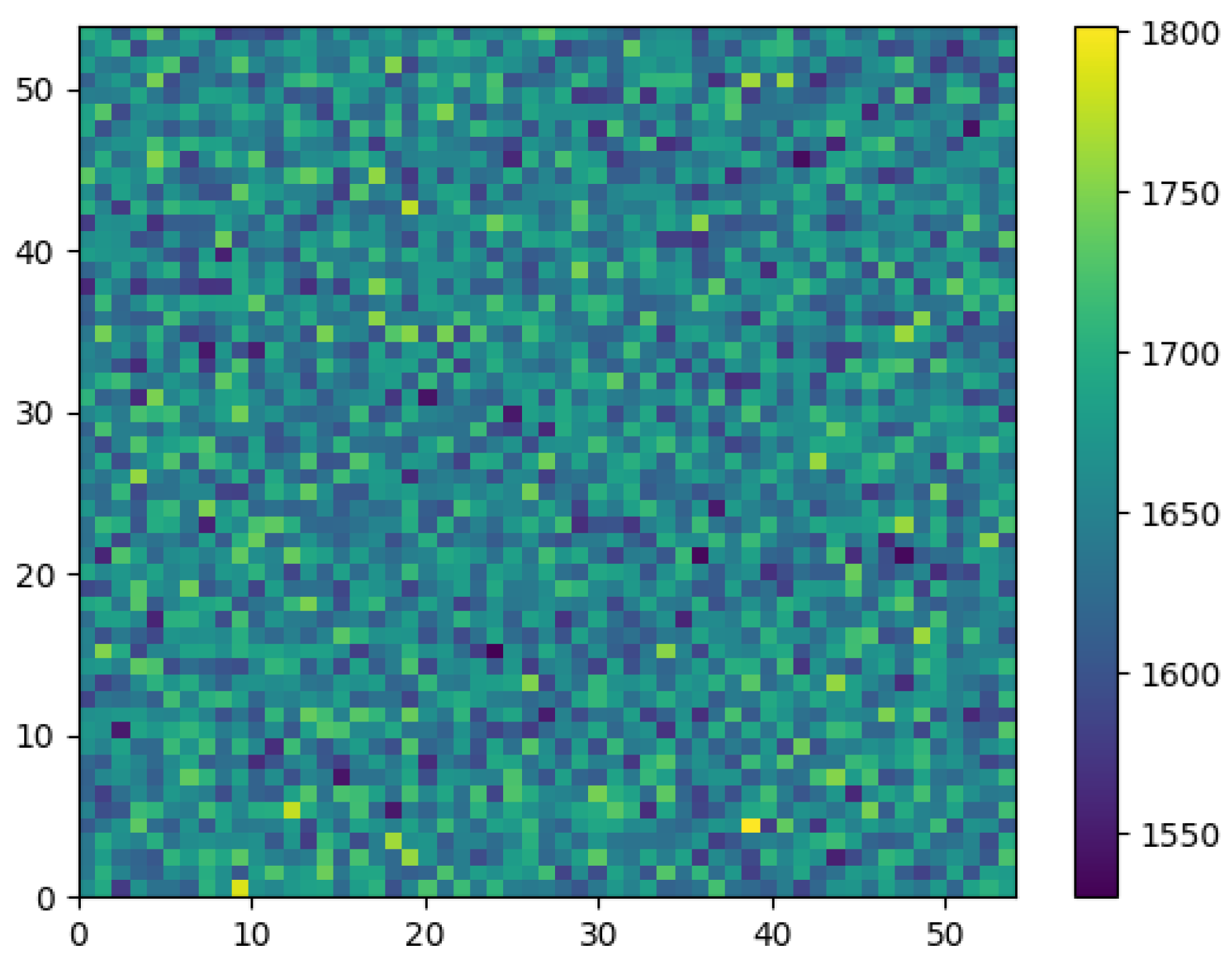
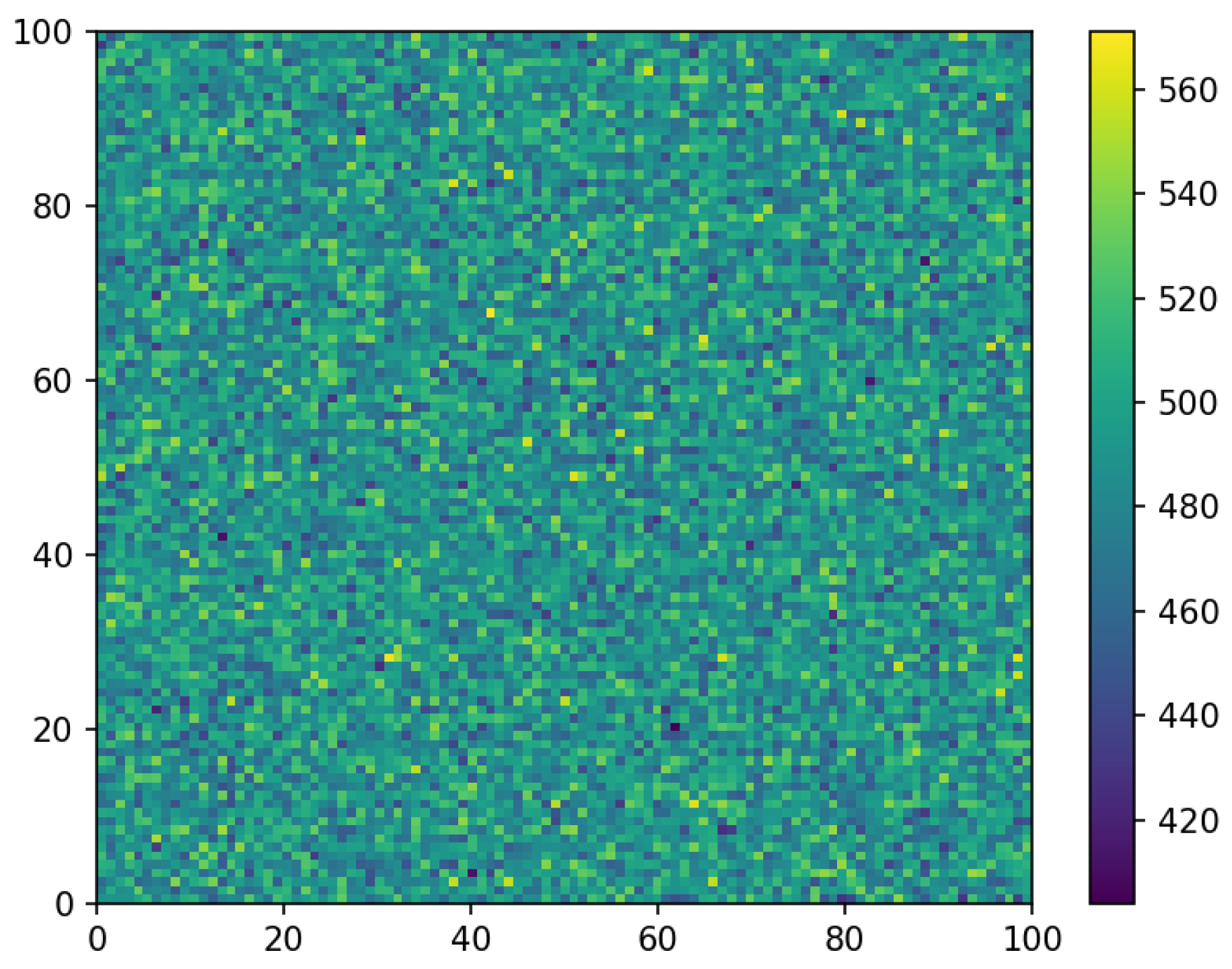
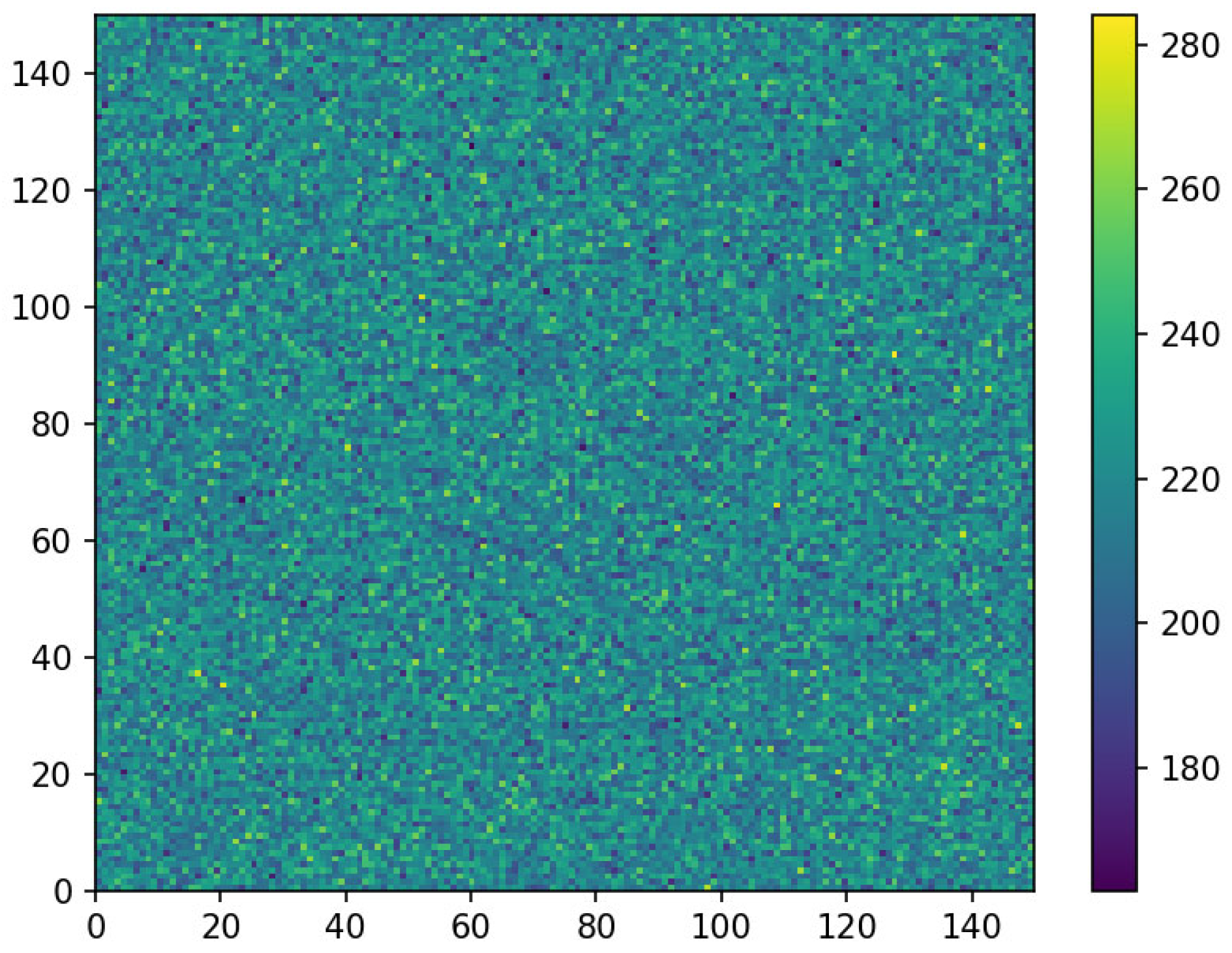
The most relevant results in the first stage of the simulation are the coordinates of the first non-conductive nodes drawn in each iteration. They show the quality of the developed algorithm. In the case of a large number of iterations, the distribution of the first non-conductive node number over the area of the square matrix should be regular.
The initial analysis of the first drawn node distribution in each of the 5 × 10
6 iterations involved the creation of two-dimensional histograms or so-called heat maps [
50]. These represent a graphical interpretation of multidimensional data, in which the individual values contained in the matrix are represented by a colour scale.
Figure 2,
Figure 3 and
Figure 4 show the corresponding colour for each node of the matrices for networks of dimensions
L = 55,
L = 101 and
L = 151. The colours represent the number of the first non-conductive nodes in each node of the matrix.
Analysis of
Figure 2,
Figure 3 and
Figure 4 did not reveal any significant inhomogeneities in the distribution. To estimate the level of homogeneity, graphs were drawn for characteristic sections of the plane. As is known, a square matrix has a fourth-order symmetry axis passing perpendicular to the matrix through its centre. For the simulation, matrixes with odd
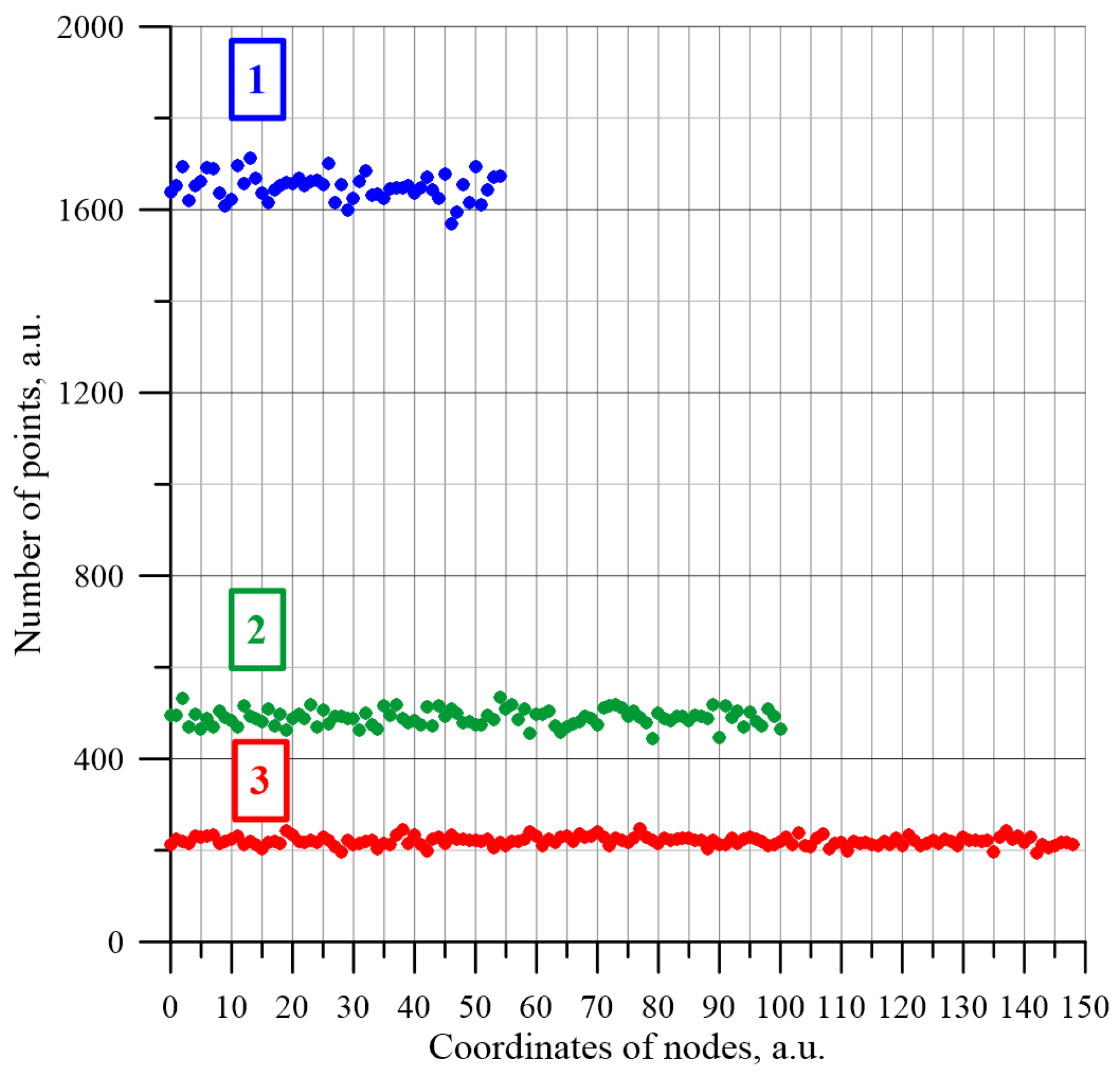
L-dimensions of 55, 101 and 151 were used to obtain a node in the centre of the matrix through which the axis of symmetry passes. This allowed us to analyse the distribution of the first non-conductive node number along lines, perpendicular to their side edges, passing through the centres of the matrixes.
Figure 5 shows a summary of the obtained results.
It can be seen from
Figure 5 that for all the matrixes analysed, the distributions are constant values. To estimate the homogeneity of the distributions shown in
Figure 5, the standard deviation values, calculated from the equation, were used:
where:
σ—standard deviation,
—mean value,
n—number of iterations,
xk—results for iteration number
k.
The standard deviation value is used in metrology to determine the type A uncertainty of measurement [
39], given by the equation:
Uncertainty of measurement is used to estimate numerical values, obtained by repeated measurements, by statistical methods. In this case, the measurement result consists of the measured value and measurement uncertainty. The measurand value in the case of repeated measurement is the arithmetic mean value of subsequent measurement results, while the uncertainty of measurement is given by Equation (4). The result of a measurement can be written in the form:
Relative uncertainty, as defined [
39], is used to compare the measurement uncertainty and the measured value:
The mean value of the first non-conductive nodes in each matrix node for matrixes with L = 55 is 1652.89, L = 101 is 490.15 and L = 151 is 219.29. Calculated from the simulation results, the type A uncertainty of measurement by Equation (4) and the relative uncertainties by Equation (6) for first nodes number are: for matrix with L = 55 u = 8.28 × 10⁻⁴ and δ = 5.01 × 10⁻⁶, matrix L = 101 u = 1.63 × 10⁻³ and δ = 3.32 × 10⁻⁶, for matrix L = 151 u = 2.94 × 10⁻³ and δ = 1.34 × 10⁻⁵. Based on these results, it can be concluded that the distribution in space of the first randomly selected non-conductive nodes is regular. This indicates the correct operation of the software developed to simulate the percolation phenomenon.
3. Simulation of the Percolation Phenomenon for a Large Number of Iterations
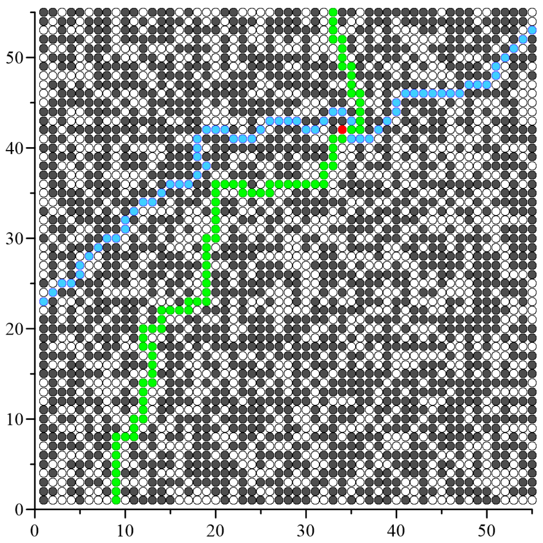
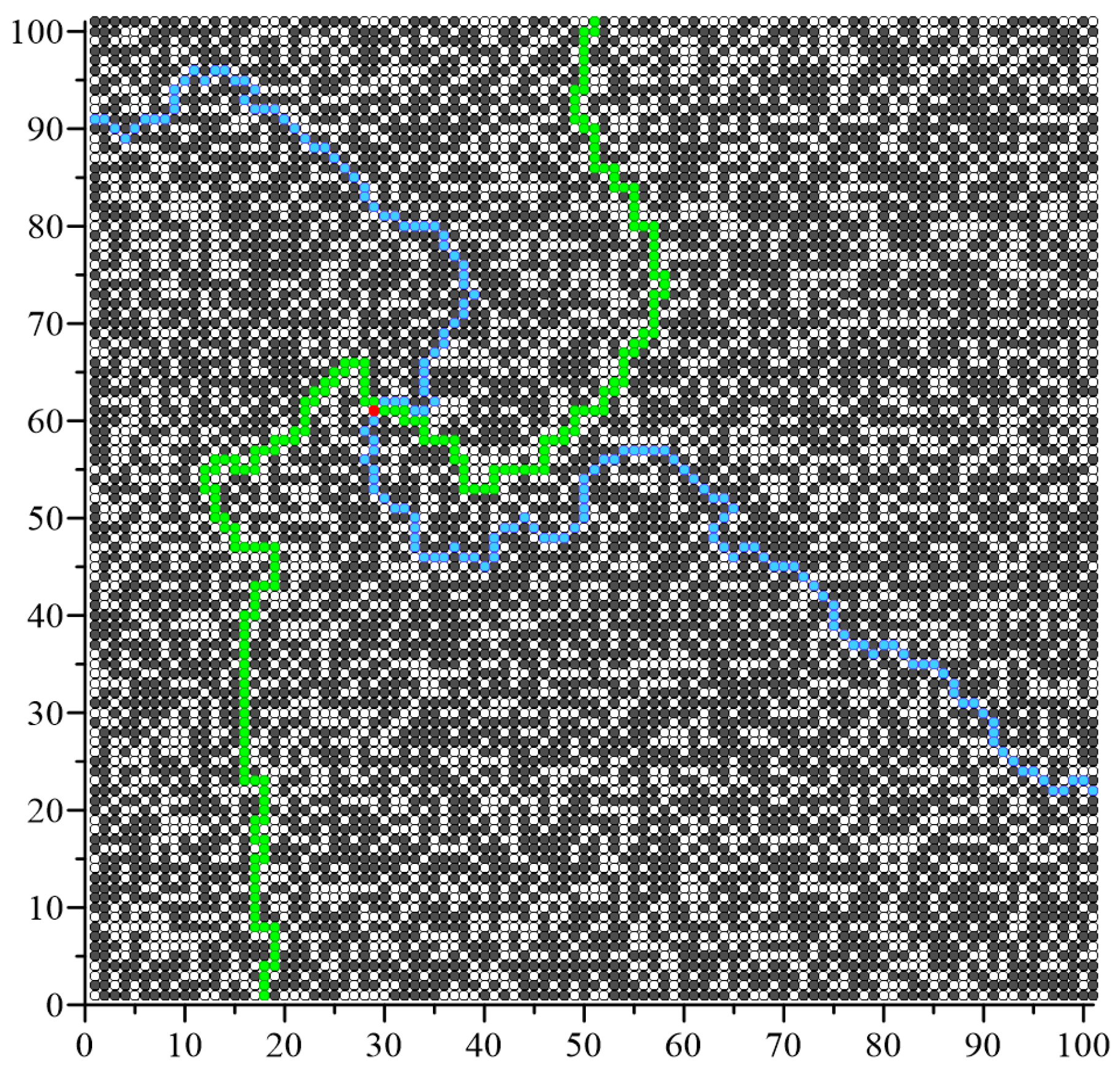
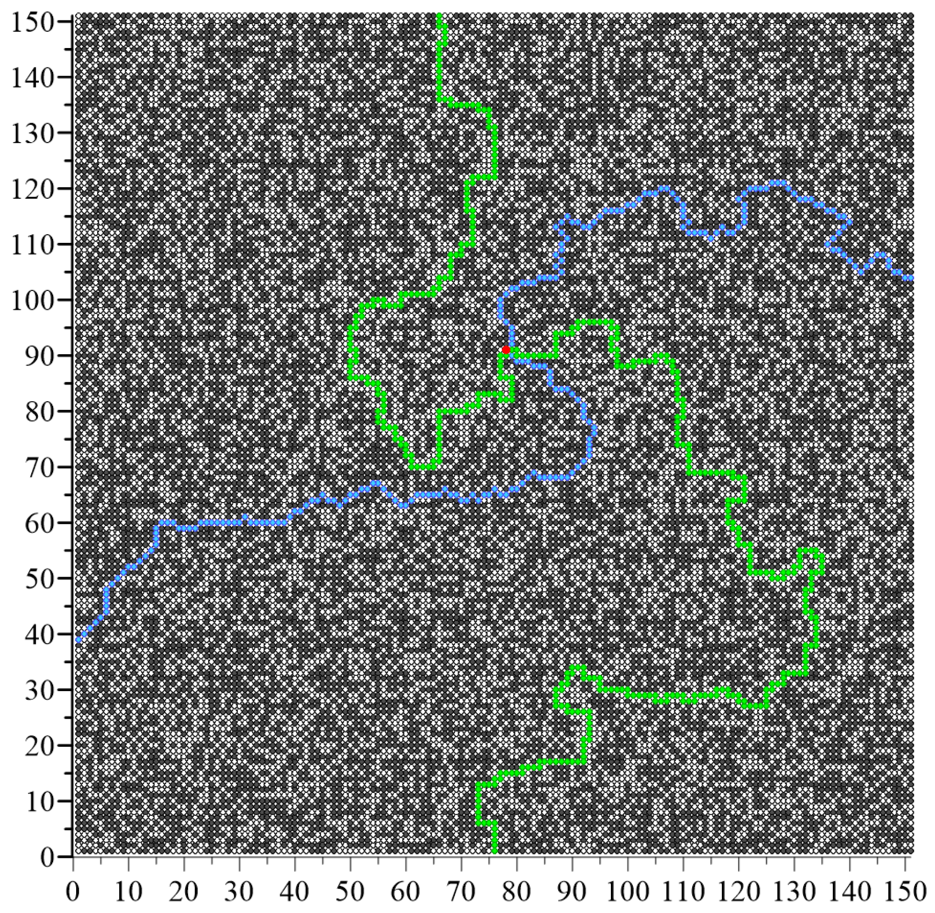
The most important simulation result was the determination of the removed conductive node number, after which the percolation threshold occurs. In the algorithm used, the last percolation channel is interrupted when the randomly drawn node marked red in
Figure 6,
Figure 7 and
Figure 8 becomes non-conductive. This creates an “infinite” non-conductive cluster that connects the two side edges of the square matrix. This node thus cuts off the current flow in the vertical direction.
Figure 6,
Figure 7 and
Figure 8 below show exemplary visualisations of simulation results for matrixes with dimensions
L = 55, 101 and 151. In the figures, black points are conducting nodes, which in the first phase of the analysis constitute 100% of the matrix nodes. Then the conducting nodes are randomly replaced by non-conducting nodes. The arrangement is defined such that the percolation edges constitute the top and bottom edges of the matrix so that the percolation threshold will be reached at the moment of interrupting the last percolation channel connecting these edges. Due to the inverted simulation logic used to optimise the analysis process, the percolation threshold is determined for the concentration in which the adjacent non-conductive nodes are connected in such a way that a non-conductive channel is created connecting the left and right edges of the tested system.
During the last iteration, a non-conductive node was drawn, marked in red, whose change in property from conductive to non-conductive determines the interruption of the last percolation channel. After drawing this node, the percolation threshold is calculated from the ratio of conducting nodes remaining in the matrix to all network nodes.
When
n independent observations have been made, for determining the percolation threshold value
xci (
i = 1, 2, …
n), and when this value varies randomly, the best achievable estimate of the expected value
is the arithmetic mean. In this case, the type A method of determining standard uncertainty should be used to determine the uncertainty of the percolation threshold estimate [
39]. In order to determine whether the percolation threshold values obtained as a result of the simulation are a random variable, histograms of the percolation threshold values distributions and their comparison with the normal distribution function for iterations number from 10
3 to 5 × 10
6 for matrixes with dimensions
L = 55, 101 and 151 were performed, as recommended in [
39]. In the simulation, the result of percolation threshold determination in each iteration is the independent variable, which is drawn from the same population. The expected value and standard deviation σ can be calculated for them. According to the central limit theorem [
51], the sequence of random variables in the form of normalised
Un values converges to a standard normal distribution for the number of iterations going to infinity and is described as:
where: σ—standard deviation,
—expected value,
n—number of iterations.
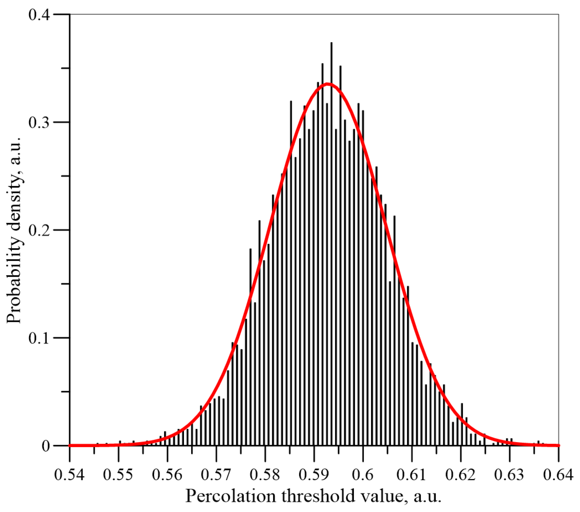
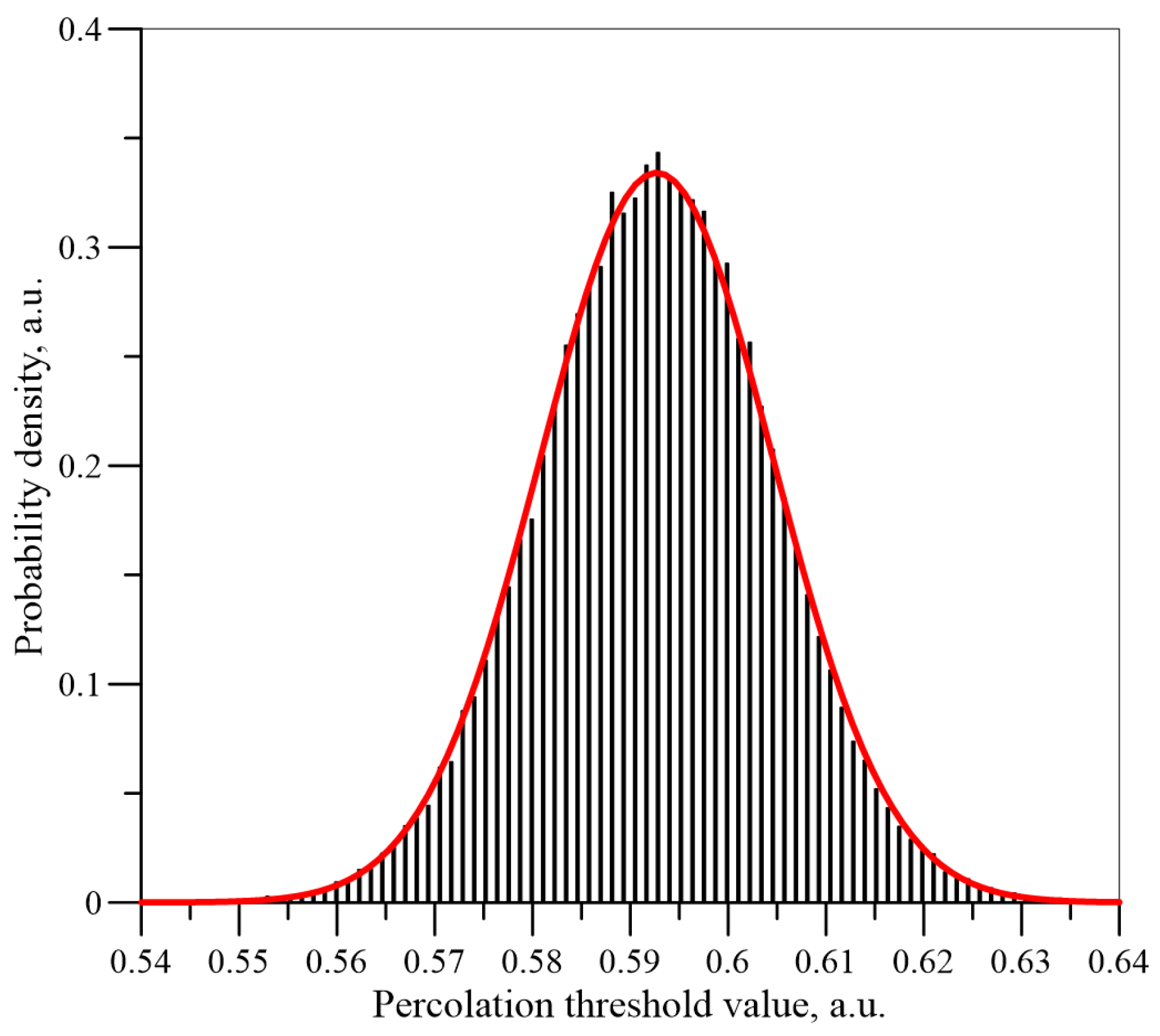
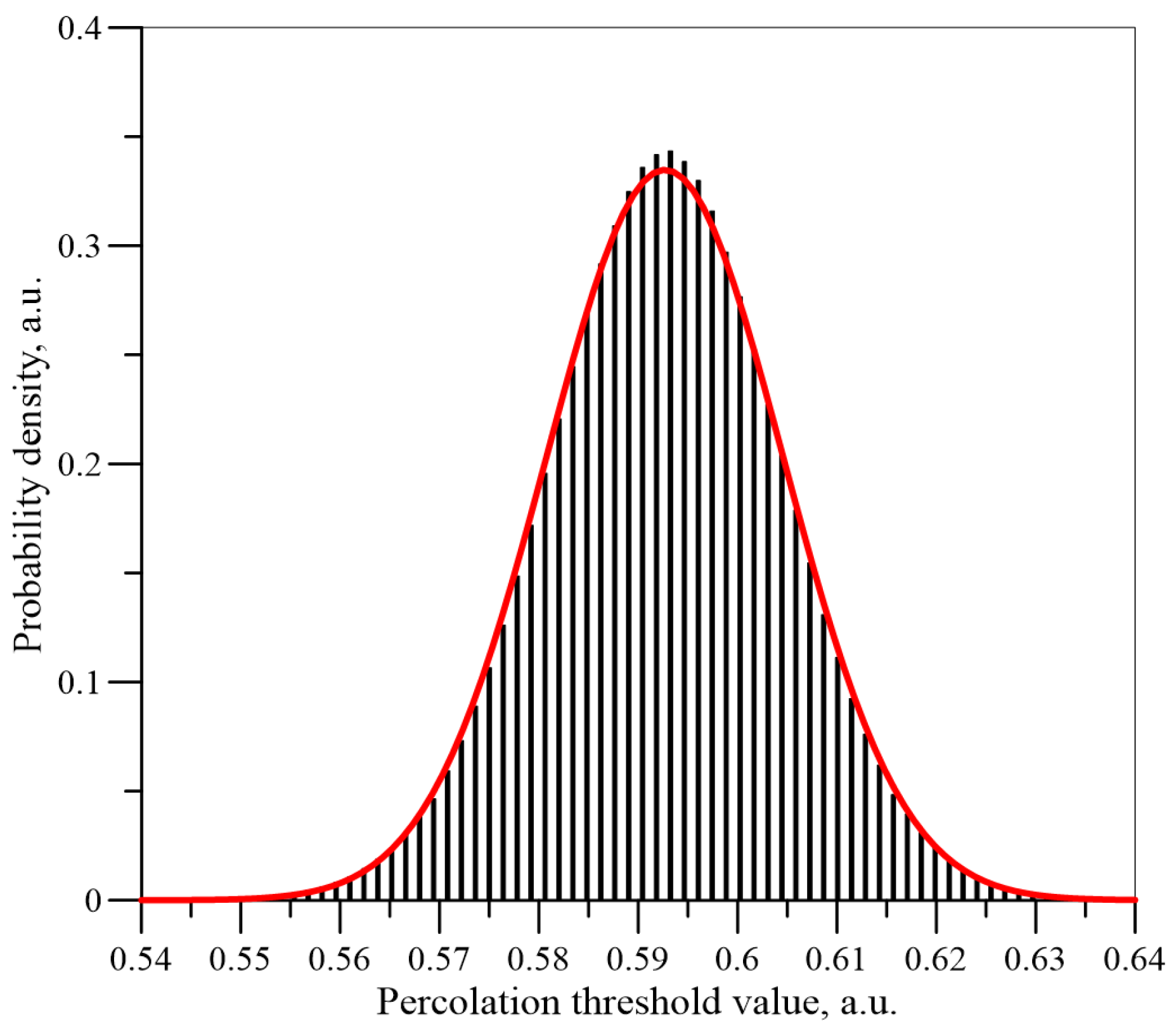
Figure 9,
Figure 10 and
Figure 11 show the histograms of the normalised
Un values dependence for the number of iterations
n = 5 × 10
3, 5 × 10
4 and 5 × 10
6 for a matrix of dimension
L = 151. The normal distributions calculated for the mean values and standard deviations, which have been determined on the basis of the simulations, are also shown in these figures.
It can be seen from
Figure 9,
Figure 10 and
Figure 11 that, as the number of iterations increases, the results are closer and closer to a normal distribution. Similar simulations and calculations were performed for matrixes with a dimension of 55 and 101 for iteration numbers up to 5 × 10
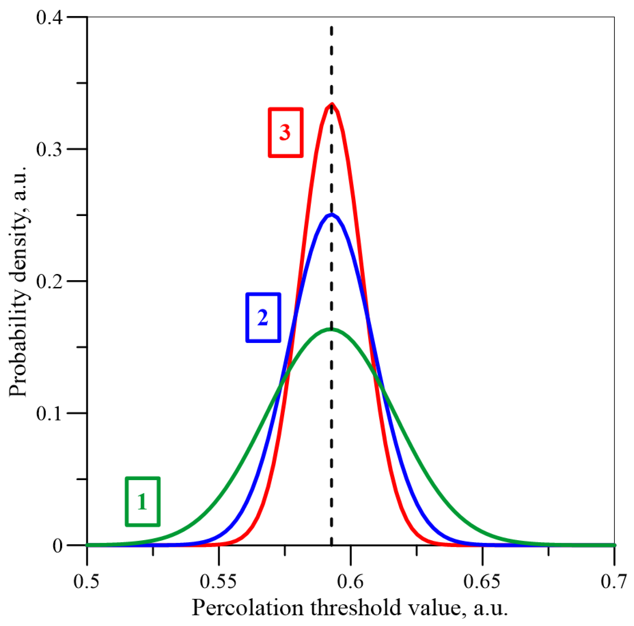
6. The results for the three matrixes are shown in
Figure 12 for iteration numbers 5 × 10
6. As can be seen from
Figure 12, as the dimensions of the matrix increase, the expected value (position of the maximum) remains constant, while the standard deviation value (width of the distribution) decreases.
The percolation threshold values obtained were compared with the density value of the normal distribution for the given values of
and
σ depending on the number of iterations and, as recommended in [
39],
R2 coefficients of determination were calculated as functions of the regression results using least squares estimation.
Table 1 summarises the coefficients of determination values for matrixes with
L = 55, 101, 151, depending on the number of iterations.
As can be seen from
Table 1, the
R2 coefficients of determination already for an iteration number of 5 × 10
4 are greater than 0.99 and very close to unity. Their values for an iteration number of 5 × 10
6 are 0.9984, 0.9990 and 0.9993 for matrixes of 55, 101 and 151, respectively. The close to unity values of the coefficients of determination demonstrate the good quality of the simulation results approximation using normal distributions. This means that the probability distribution of nodes interrupting the last percolation channel is a normal distribution and the percolation threshold value is a random variable. This allows the type A method of determining the uncertainty given by Equation (4) [
39] to be used to determine the uncertainty in the estimation of percolation thresholds later in the article.
The dependencies of the normal distribution basic parameters—the mean value of the percolation threshold and the standard deviation on the number of iterations
n—were determined. Successive values of the iteration number for which calculations were made were determined using the equation:
where:
n—integer part of a number, enclosed in square brackets,
m = 0, 1, 2, 3 ... This choice of iteration number allows them to be evenly distributed on a logarithmic scale.
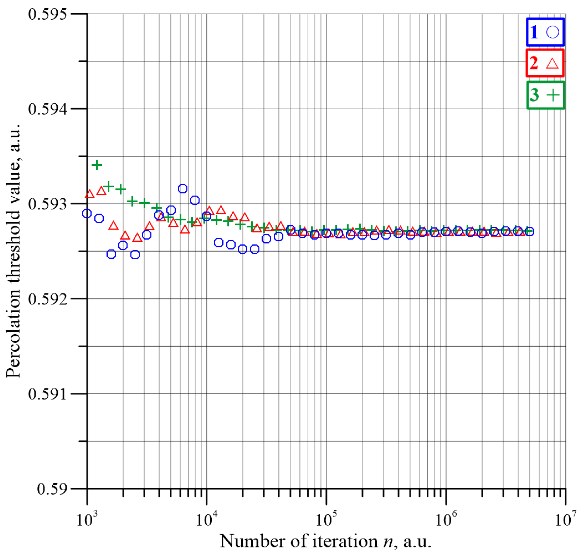
Figure 13 shows the dependence of the average percolation threshold value on the number of iterations for matrixes of dimensions 55, 101 and 151. The figure shows every fifth number of iterations value. It can be seen from the figure that for a relatively small iteration number, the percolation threshold values change over a small range, not exceeding 0.0007. For iteration numbers of 5 × 10
4 and above, the percolation threshold values change in the range below 10
−4 and gradually stabilise. This means that, for large numbers of iterations, the percolation threshold value hardly depends on the dimensions of the matrix.
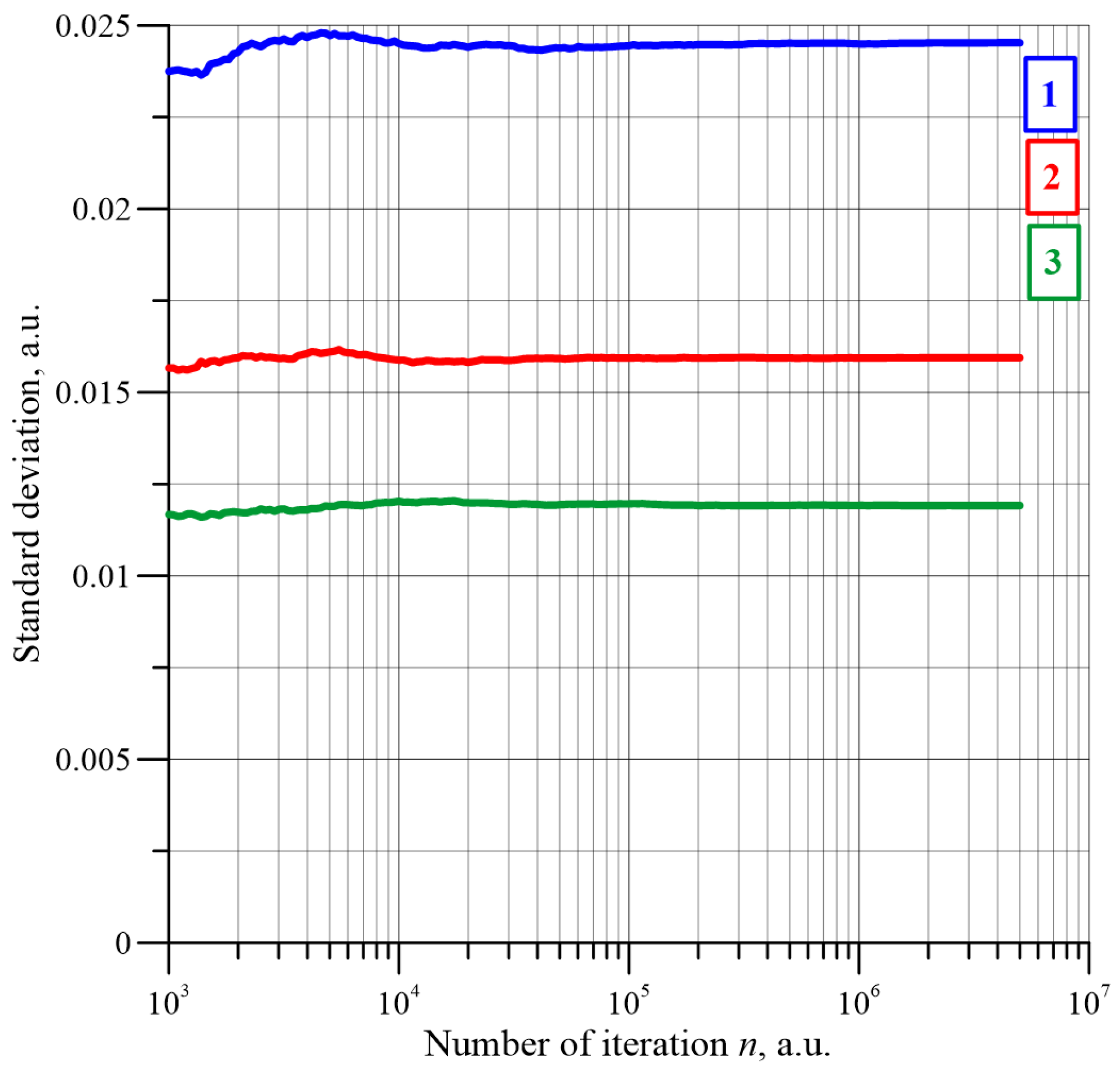
Figure 14 shows the waveforms of standard deviation as a function of the iteration number. For a small number of iterations, some variation in the standard deviation values is apparent. Once the number of iterations exceeds approximately 5 × 10
4 and above, the standard deviation values practically stabilise.
It should be noted that
Figure 14 shows that the value of the standard deviation for a large number of iterations decreases as the dimensions of the matrix increase. For iteration number values of 5 × 10
6, the following standard deviation values were obtained: 0.024526293 for a matrix with
L = 55, 0.015941405—
L = 101, 0.011915908—
L = 151. Based on the standard deviation values obtained for the number of iterations 5 × 10
6, the percolation threshold estimation values and the relative uncertainty for matrixes with dimensions
L = 51, 101, 151 were calculated using Equations (4) and (6). The calculation resulted in the following percolation thresholds:
xc(
L = 55) ≈ (0.5927046 ± 1.1 × 10
−5), relative uncertainty δ(
L = 55) ≈ 1.9 × 10
−5,
xc(
L = 101) ≈ (0.5927072 ± 7.13 × 10
−6), δ(
L = 101) ≈ 1.2 × 10
−5,
xc(
L = 151) ≈ (0.5927135 ± 5.33 × 10
−6), δ(
L = 151) ≈ 8.99 × 10
−6. From a comparison of the results, shown in
Figure 13 and
Figure 14, for large iteration numbers the percolation threshold values are almost independent of the matrix dimensions. The standard deviations for large iteration numbers hardly depend on the number of iterations, while the values of standard deviation decrease as the dimensions of the matrix increase.
Figure 9,
Figure 10,
Figure 11,
Figure 12,
Figure 13 and
Figure 14 show that increasing the number of iterations to very large values for a matrix of specific dimensions leaves the normal probability distribution of percolation threshold values virtually unchanged. This distribution is described by two parameters—the mean value of the percolation threshold and the standard deviation.
From Equation (4), it follows that the uncertainty in the percolation threshold estimation is proportional to the value of the standard deviation and inversely proportional to the square root of the iteration number.
Figure 14 shows that the range of relatively low iteration number values should not be used to estimate the percolation threshold determination uncertainty. This is due to two factors. Firstly, the largest fluctuations in standard deviation values occur in the range of iteration numbers below 10
4. Secondly, in this area, the square root values are relatively small compared to the value for the maximum iteration number of 5 × 10
6. This means that the uncertainty values for an iteration number range below 10
4 are unsatisfactory and should be disregarded.
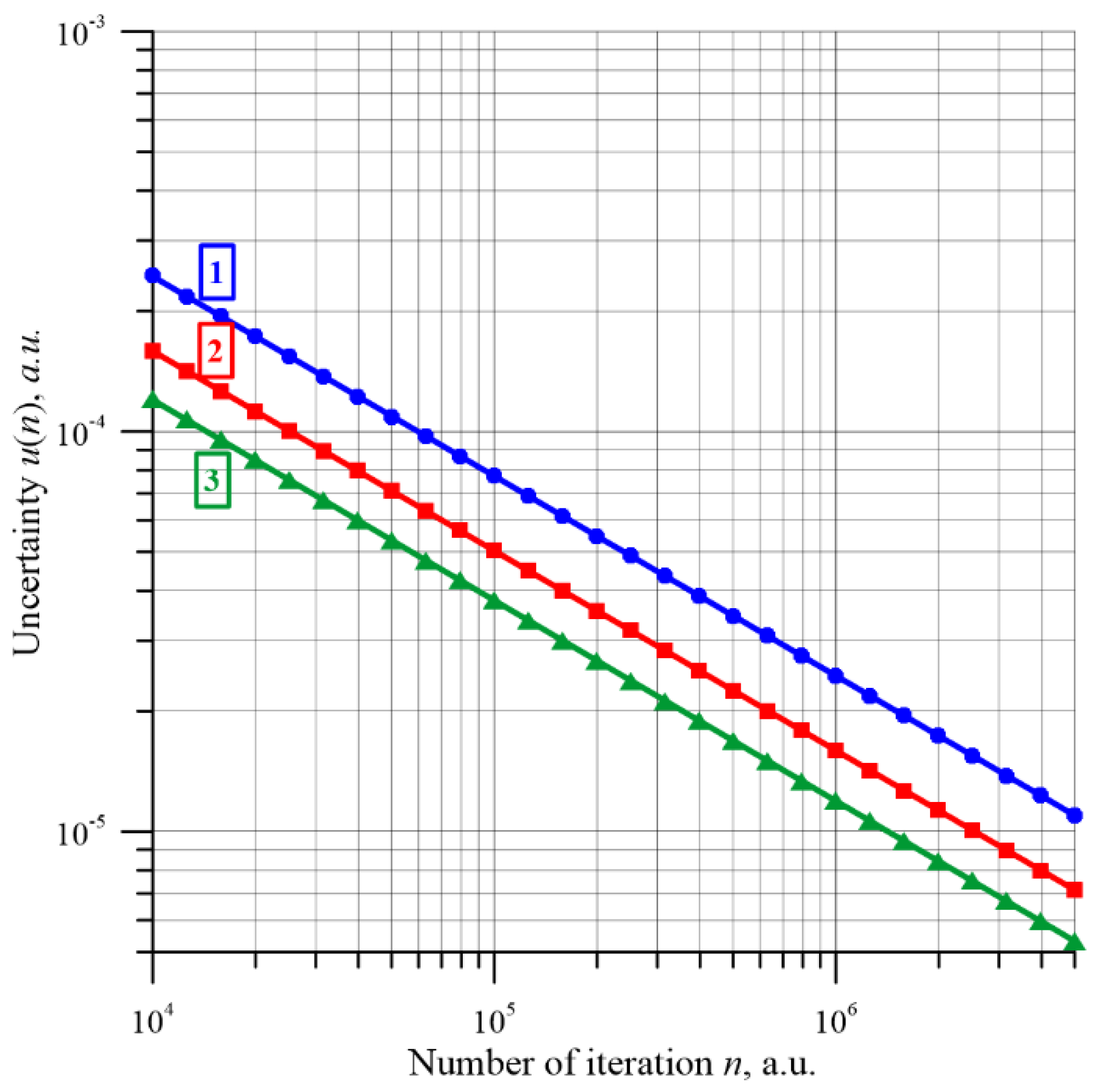
Figure 15 shows the dependence of the percolation threshold determination uncertainty on the number of iterations for matrixes of dimensions 55, 101 and 151, calculated according to Equation (4) for a range of iterations numbers from 10
4 to 5 × 10
6. This figure also shows the approximation waveforms in the form of power functions.
The following conclusions emerge from the analysis of
Figure 15. The
R2 determination coefficients for the approximation waveforms are very close to unity and are 0.999981761, 0.99997486 and 0.99995301 for matrixes with
L = 55, 101 and 151, respectively. The differences between them and unity are no more than 0.00007815. This indicates a very good approximation of the simulation results. As is well known, the dependence of uncertainty on the number of iterations is described, by definition, by the equation [
39], which can be presented in the form:
where:
σ—standard deviation,
n—number of iterations.
From the approximations, shown in
Figure 15, it follows that the experimental dependencies
uD(
n) are described by the equation:
where:
uD—uncertainty of the percolation threshold estimate,
σD—experimental value of the standard deviation,
n—number of iterations,
k—power factor.
For matrixes with
L = 55, 101 and 151, the following approximation equations were obtained:
Equations (11)–(13) show that the experimental power coefficients are very close to the value—0.5. The largest difference between the power value in Equation (9) and the coefficients from the approximating Equations (11)–(13) occurs for the matrix with L = 151 and is only about 0.00264917. For the other matrixes, the differences are even smaller.
In Equations (11)–(13), the numerical coefficients in front of the iterations number
n are the standard deviation values, determined from the simulation results approximations of the type A uncertainty dependence on the number of iterations. These values were also calculated directly from 5 × 10
6 iterations (see
Figure 13 and
Figure 15). The comparison of pairs of standard deviation values determined directly and from the approximation gives the following differences between them: Δ
σ(
L = 55) = 0.00045110, Δ
σ(
L = 101) = 0.00015160, Δ
σ(
L = 151) = 0.00037728. The comparison of these differences shows that the values of standard deviations determined directly and from the approximation are very close to each other. This means that the dependencies of the percolation threshold value uncertainty estimation on the number of iterations, obtained by approximation of the simulation results acquired with the Monte Carlo method perfectly agree with the definition of type A uncertainty [
39]. This is evidenced by both the power values, very close to −0.5, and the values of standard deviations. Comparing the results of the approximations with Equation (9), it should be noted that for a matrix of specific dimensions, the uncertainty in the estimation of the percolation threshold is a function of the number of iterations only, and the value of the standard deviation σ does not depend on the number of iterations for
n ≥ 104. This means that a reduction in the uncertainty of the percolation threshold determination for a matrix of certain dimensions is only possible by increasing the number of iterations.
It can be seen from
Figure 15 that an increase in the matrix dimensions decreases the uncertainty, leaving the power relationship unchanged. This is associated, according to Equations (11)–(13), with a decrease in the standard deviation, as the matrix dimensions increase, which is also visible in
Figure 14. The reduction in the standard deviation value established in the study with an increase in the matrix dimensions allowed us to propose a method to reduce the uncertainty in the percolation threshold estimation not only by increasing the number of iterations but also by increasing the dimensions of the matrix. For example, to reduce the uncertainty in the estimation of the percolation threshold by an order of magnitude for a matrix with
L = 55, that is, from 1.1 × 10
−5 to 1.1 × 10
−6, requires, according to Equation (9), a hundredfold increase in the number of iterations from 5 × 10
6 to 5 × 10
8.
Figure 15 shows that the reduction of the uncertainty value along with the increase in matrix dimensions makes it possible to apply the uncertainty reduction method, consisting of increasing the dimensions of the matrix. For example, the uncertainty in estimating the percolation threshold for a matrix with
L = 55 and an iteration number of 5 × 10
6 is 1.1 × 10
−5. The same uncertainty for the matrix with
L = 151 will be obtained after about 4.166 times the smaller number of iterations of about 1.2 × 10
6.
This means that based on the data obtained in the work, it is possible to optimise the determination of percolation threshold estimation uncertainty based on the use of the metrological approach. Optimisation consists of selecting the dimensions of the matrix and the number of iterations in order to obtain the assumed uncertainty of the percolation threshold determination. The proposed optimisation procedure can be used to simulate the percolation phenomena of both nodes and bonds in a matrix with shapes and symmetry types other than square matrixes.


 ,
, 


