
Numerical Modeling of PD Pulses Formation in a Gaseous Void Located in XLPE Insulation of a Loaded HVDC Cable


Abstract
:1. Introduction
- submarine electrical energy transmission [4].
- -
- Gaseous voids;
- -
- Delaminations;
- -
- Protrusions;
- -
- Contaminations;
- -
- Electrical trees;
- -
- Water trees.
2. The Problem of PD Formation and the Numerical Model of the DC Cable
2.1. PD Formation in Gaseous Void—Overview
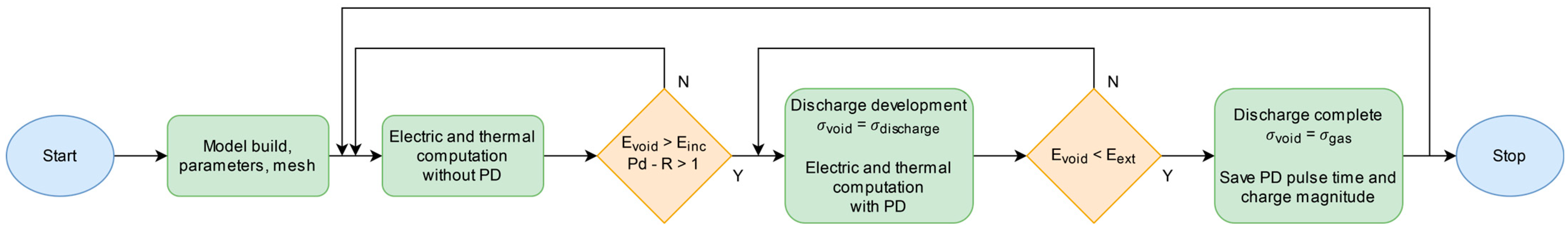
- (1)
- The electric field strength in the void must exceed the value of the discharge inception field strength;
- (2)
- As a result of volume or surface processes, an initial electron must be present to trigger the development of the discharge process.
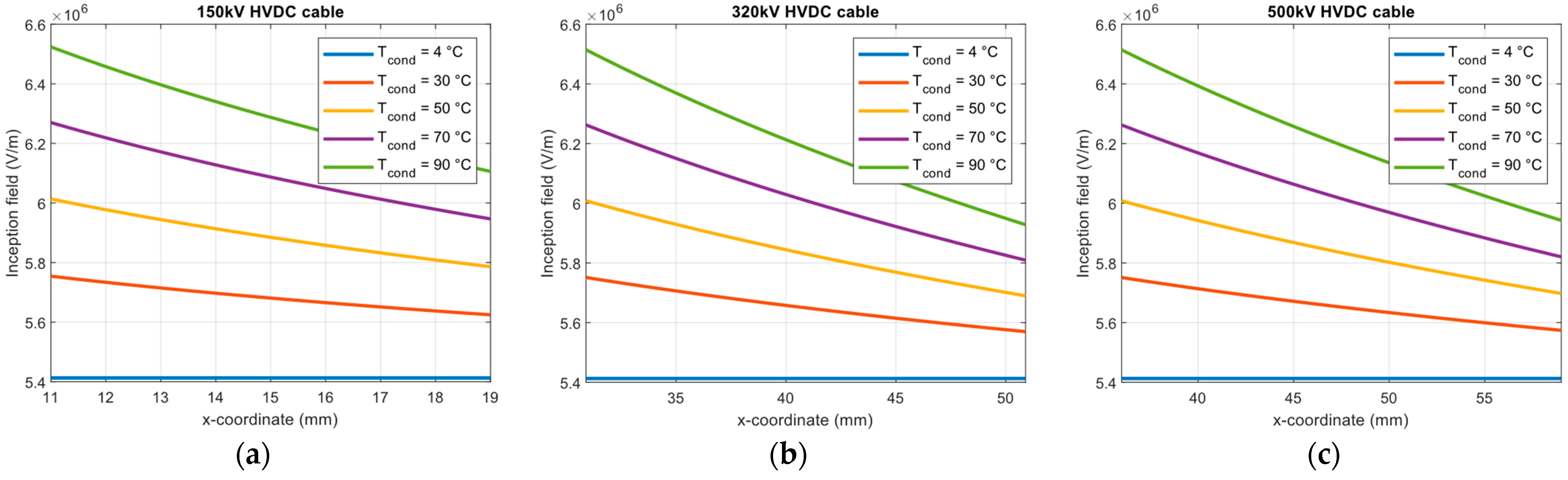
- Einc—PD inception field strength, V·m−1;
- (E/p)cr—critical electric field to pressure ratio, for air 25.2 [V·m−1·Pa−1];
- p—gas pressure in void [Pa];
- d—gaseous void dimension (the void diameter or height parallel to the applied E field) [m];
- B, n—ionization process coefficients (for air B = 8.6 [m1/2·Pa1/2], n = 0.5).
- Evoid—electric field strength in a gaseous void, V·m−1;
- τlag—PD inception lag time, s;
- ∆tinc—the period of time counted from the moment when the field strength in the void Evoid exceeded the Einc, s.
- Eext—the PD extinction field strength, V·m−1;
- Ecr—the critical field strength, V·m−1;
- χ—the PD extinction field coefficient, -.
2.2. Electric Field in Model HVDC Cable Insulation
- σ0—specific dielectric conductivity, S·m−1 (at E = 0.0 V·m−1 and T = 0 °C);
- T—temperature, °C;
- E—electric field strength, V·m−1;
- α—temperature factor of conductivity, °C−1;
- β—field factor of conductivity, V−1·m.
- A, B— specific factors for the dielectric;
- φ—thermal activation energy, eV;
- qe—elementary charge;
- T—temperature, K;
- E—electric field strength, V·m−1.
2.3. Cable Model for E Field Analysis with Finite Element Method
3. Simulation Results—Case Studies for Three Model Cables
- -
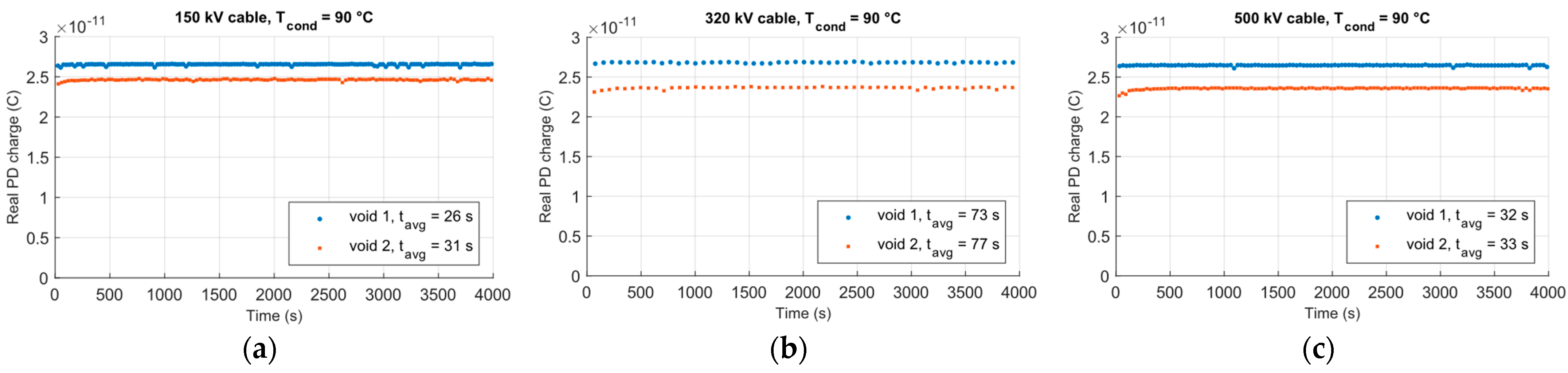
- Average PD magnitude qav, pC;
- -
- Average time interval between successive PD pulses ∆tav, s.
4. Discussion
- (a)
- On the inner radius of the insulation xmin
- -
- For 150 kV cable, from 12.7 kV·mm−1 to 21.3 kV·mm−1;
- -
- For 320 kV cable, from 7.8 kV·mm−1 to 18.1 kV·mm−1;
- -
- For 500 kV cable, from 12.2 kV·mm−1 to 24.2 kV·mm−1.
- (b)
- On the outer radius of the insulation
- -
- For 150 kV cable, from 16.7 kV·mm−1 to 24.3 kV·mm−1;
- -
- For 320 kV cable, from 14.3 kV·mm−1 to 24.4 kV·mm−1;
- -
- For 500 kV cable, from 19.7 kV·mm−1 to 30.9 kV·mm−1.
- Zone I, closer to the cable core, limited by xmin and xc radii;
- Zone II, closer to the outer screen on the insulation, limited by xc and xmax radii.
- kV—zone volume factor, %;
- xmin—inner radius of insulation, mm;
- xmax—outer radius of insulation, mm;
- xc—radius of the insulation layer with (almost) constant E field, mm.
5. Conclusions
- Reference of the conditions of PD formation in XLPE insulation of ‘cold’ and ‘hot’ HVDC cables to the location of the gaseous void on the cable radius; these analyses concerned three different designs of HVDC cables, but their results can be generalized;
- Simulating and analyzing the parameters of the sequence of PD pulses generated independently in two PD sources with different locations on the cable radius;
- Distinguishing two zones in the HVDC cable where the conditions of PD formation in the ‘cold’ and ‘hot’ cable insulation are different due to the radial temperature distribution and ‘normal’ or ‘inverted’ electric field distribution;
- Estimation of the critical dimension of the gaseous void depending on the position and thermal condition of the cable insulation, for each of the analyzed projects.
Author Contributions
Funding
Data Availability Statement
Conflicts of Interest
References
- Humpert, C. Long distance transmission systems for the future electricity supply—Analysis of possibilities and restrictions. Energy 2012, 48, 278–283. [Google Scholar] [CrossRef]
- Hammons, T.J.; Lescale, V.F.; Uecker, K.; Haeusler, M.; Retzmann, D.; Staschus, K.; Lepy, S. State of the art in ultrahigh-voltage transmission. Proc. IEEE 2012, 100, 360–390. [Google Scholar] [CrossRef]
- Zhou, H.; Qiu, W.; Sun, K.; Chen, J.; Deng, X.; Qian, F.; Wang, D.; Zhao, B.; Li, J.; Li, S.; et al. (Eds.) Ultra-High Voltage AC/DC Power Transmission; Springer: Berlin/Heidelberg, Germany, 2019. [Google Scholar]
- Worzyk, T. Submarine Power Cables Design, Installation, Repair, Environmental Aspects; Springer: Berlin/Heidelberg, Germany, 2009. [Google Scholar]
- Mazzanti, G.; Marzinotto, M. Extruded Cables for High-Voltage Direct-Current Transmission: Advances in Research and Development; Wiley-IEEE Press: Hoboken, NJ, USA, 2013. [Google Scholar]
- Jovcic, D.; Ahmed, K. High-Voltage Direct-Current Transmission. Converters, Systems and DC Grids; John Wiley & Sons: Hoboken, NJ, USA, 2015. [Google Scholar]
- Liu, R. Long-distance DC electrical power transmission. IEEE Electr. Insul. Mag. 2013, 29, 37–46. [Google Scholar] [CrossRef]
- Alassi, A.; Bañales, S.; Ellabban, O.; Adam, G.; MacIver, C. HVDC transmission: Technology review, market trends and future outlook. Renew. Sustain. Energy Rev. 2019, 112, 530–554. [Google Scholar] [CrossRef]
- Li, Z.; Song, Q.; An, F.; Zhao, B.; Yu, Z.; Zeng, R. Review on DC transmission systems for integrating large-scale offshore wind farms. Energy Convers. Econ. 2021, 2, 1–14. [Google Scholar] [CrossRef]
- Acaroğlu, H.; Márquez, F.P.G. High voltage direct current systems through submarine cables for offshore wind farms: A life-cycle cost analysis with voltage source converters for bulk power transmission. Energy 2022, 249, 123713. [Google Scholar] [CrossRef]
- ENTSO-E. HVDC Links in System Operations, European Network of Transmission System Operators for Electricity; Technical Paper; ENTSO-E: Brussels, Belgium, 2019. [Google Scholar]
- Stan, A.; Costinaș, S.; Ion, G. Overview and assessment of HVDC current applications and future trends. Energies 2022, 15, 1193. [Google Scholar] [CrossRef]
- Parol, M.; Robak, S.; Rokicki, Ł.; Wasilewski, J. Cable links designing in HVAC and HVDC submarine power grids—Selected issues. Prz. Elektrotech. 2019, 95, 7–13. [Google Scholar] [CrossRef]
- Li, Y.; Liu, H.; Fan, X.; Tian, X. Engineering practices for the integration of large-scale renewable energy VSC-HVDC systems. Glob. Energy Interconnect. 2020, 3, 149–157. [Google Scholar] [CrossRef]
- Offshore Transmission Technology; Report of ENTSO-E’s Regional Group North Sea; European Network of Transmission System Operators for Electricity: Brussels, Belgium, 2011.
- Stone, G.C.; Boulter, E.A.; Culbert, I.; Dhirani, H. Electrical Insulation for Rotating Machines: Design, Evaluation, Aging, Testing, and Repair, 1st ed.; Wiley-IEEE Press: Milwaukee, WI, USA, 2004. [Google Scholar]
- IEC 60505:2011; Evaluation and Qualification of Electrical Insulation Systems. IEC: Genève, Switzerland, 2011.
- Dissado, L.A.; Fothergill, J.C. Electrical Degradation and Breakdown in Polymers; Peregrinus Press: Chicago, IL, USA, 1992. [Google Scholar]
- Jones, J.P.; Llewellyn, J.P.; Lewis, T.J. The contribution of field-induced morphological change to the electrical aging and breakdown of polyethylene. IEEE Trans. Dielectr. Electr. Insul. 2005, 12, 951–966. [Google Scholar] [CrossRef]
- Marzinotto, M.; Mazzanti, G. The statistical enlargement law for HVDC cable lines part 1: Theory and application to the enlargement in length. IEEE Trans. Dielectr. Electr. Insul. 2015, 22, 192–201. [Google Scholar] [CrossRef]
- Montanari, G.C.; Seri, P.; Dissado, L.A. Aging mechanisms of polymeric materials under DC electrical stress: A new approach and similarities to mechanical aging. IEEE Trans. Dielectr. Electr. Insul. 2019, 26, 634–641. [Google Scholar] [CrossRef]
- Montanari, G.C.; Morshuis, P.; Seri, P.; Ghosh, R. Ageing and reliability of electrical insulation: The risk of hybrid AC/DC grids. High Volt. 2020, 5, 620–627. [Google Scholar] [CrossRef]
- Naderiallaf, H.; Seri, P.; Montanari, G.C. Designing a HVDC insulation system to endure electrical and thermal stresses under operation. Part I: Partial discharge magnitude and repetition rate during transients and in DC steady state. IEEE Access 2021, 9, 35730–35739. [Google Scholar] [CrossRef]
- Cambareri, P.; de Falco, C.; Rienzo, L.D.; Seri, P.; Montanari, G.C. Electric field calculation during voltage transients in HVDC cables: Contribution of polarization processes. IEEE Trans. Power Deliv. 2022, 37, 5425–5432. [Google Scholar] [CrossRef]
- Lei, Z.; Song, J.; Tian, M.; Cui, X.; Li, C.; Wen, M. Partial discharges of cavities in ethylene propylene rubber insulation. IEEE Trans. Dielectr. Electr. Insul. 2014, 21, 1647–1659. [Google Scholar] [CrossRef]
- Alshaikh Saleh, M.; Refaat, S.S.; Olesz, M.; Abu-Rub, H.; Guziński, J. The effect of protrusions on the initiation of partial discharges in XLPE high voltage cables. Bull. Pol. Acad. Sci. Tech. Sci. 2021, 69, e136037. [Google Scholar] [CrossRef]
- Dissado, L.A.; Dodd, S.J.; Champion, J.V.; Williams, P.I.; Alison, J.M. Propagation of electrical tree structures in solid polymeric insulation. IEEE Trans. Dielectr. Electr. Insul. 1997, 4, 259–279. [Google Scholar] [CrossRef]
- Chen, X.; Mantsch, A.R.; Hu, L.; Gubanski, S.M.; Blennow, J.; Olsson, C.O. Electrical treeing behavior of DC and thermally aged polyethylenes utilizing wire-plane electrode geometries. IEEE Trans. Dielectr. Electr. Insul. 2014, 21, 45–52. [Google Scholar] [CrossRef]
- Ross, R. Inception and propagation mechanisms of water treeing. IEEE Trans. Dielectr. Electr. Insul. 1998, 5, 660–680. [Google Scholar] [CrossRef]
- Li, J.; Zhao, X.; Yin, G.; Li, S.; Zhao, J.; Ouyang, B. The effect of accelerated water tree ageing on the properties of XLPE cable insulation. IEEE Trans. Dielectr. Electr. Insul. 2011, 8, 1562–1569. [Google Scholar] [CrossRef]
- Fard, M.A.; Farrag, M.E.; McMeekin, S.; Reid, A. Electrical treeing in cable insulation under different HVDC operational conditions. Energies 2018, 11, 2406. [Google Scholar] [CrossRef]
- Liu, H.; Zhang, M.; Liu, Y.; Xu, X.; Liu, A. Growth and partial discharge characteristics of DC electrical trees in cross-linked polyethylene. IEEE Trans. Dielectr. Electr. Insul. 2019, 26, 1965–1972. [Google Scholar] [CrossRef]
- Liu, F.; Rowland, S.M.; Zheng, H.; Peesapati, V. Electrical tree growth in LDPE: Fine channel development during negative DC ramp down. IEEE Trans. Dielectr. Electr. Insul. 2022, 29, 1218–1220. [Google Scholar] [CrossRef]
- Drissi-Habti, M.; Raj-Jiyoti, D.; Vijayaraghavan, S.; Fouad, E.-C. Numerical Simulation for Void Coalescence (Water Treeing) in XLPE Insulation of Submarine Composite Power Cables. Energies 2020, 13, 5472. [Google Scholar] [CrossRef]
- Miceli, M.; Carvelli, V.; Drissi-Habti, M. Modelling electro-mechanical behaviour of an XLPE insulation layer for Hi-Voltage composite power cables: Effect of voids on onset of coalescence. Energies 2023, 16, 4620. [Google Scholar] [CrossRef]
- Chen, G.; Davies, A.E. The influence of defects on the short-term breakdown characteristics and long-term dc performance of LDPE insulation. IEEE Trans. Dielectr. Electr. Insul. 2000, 7, 401–407. [Google Scholar] [CrossRef]
- Mazzanti, G.; Montanari, G.C.; Civenni, F. Model of inception and growth of damage from microvoids in polyethylene-based materials for HVDC cables—Part 1: Theoretical approach. IEEE Trans. Dielectr. Electr. Insul. 2007, 14, 1242–1254. [Google Scholar] [CrossRef]
- Mazzanti, G.; Montanari, G.C.; Civenni, F. Model of inception and growth of damage from microvoids in polyethylene-based materials for HVDC cables. 2. Parametric Investigation and Data Fitting. IEEE Trans. Dielectr. Electr. Insul. 2007, 14, 1255–1263. [Google Scholar] [CrossRef]
- Niemeyer, L. A generalized approach to partial discharge modeling. IEEE Trans. Dielectr. Electr. Insul. 1995, 2, 510–528. [Google Scholar] [CrossRef]
- Pan, C.; Chen, G.; Tang, J.; Wu, K. Numerical modeling of partial discharges in a solid dielectric-bounded cavity: A review. IEEE Trans. Dielectr. Electr. Insul. 2019, 26, 981–1000. [Google Scholar] [CrossRef]
- Zhan, Y.; Chen, G.; Hao, M.; Pu, L.; Zhao, X.; Sun, H.; Wang, S.; Guo, A.; Liu, J. Comparison of two models on simulating electric field in HVDC cable insulation. IEEE Trans. Dielectr. Electr. Insul. 2019, 26, 1107–1115. [Google Scholar] [CrossRef]
- Kumara, S.; Serdyuk, Y.V.; Jeroense, M. Calculation of electric fields in HVDC cables: Comparison of different models. IEEE Trans. Dielectr. Electr. Insul. 2012, 28, 1070–1078. [Google Scholar] [CrossRef]
- Eoll, C.K. Theory of stress distribution in insulation of high-voltage DC cables: Part I. IEEE Trans. Electr. Insul. 1975, EI-10, 27–35. [Google Scholar] [CrossRef]
- Buller, F.H. Calculation of electrical stresses in DC cable insulation. IEEE Trans. Power Appar. Syst. 1967, PAS-86, 1169–1178. [Google Scholar] [CrossRef]
- Baferani, M.A.; Shahsavarian, T.; Li, C.; Tefferi, M.; Jovanovic, I.; Cao, Y. Electric field tailoring in HVDC cable joints utilizing electro-thermal simulation: Effect of field grading materials. In Proceedings of the 2020 IEEE Electrical Insulation Conference (EIC), Knoxville, TN, USA, 22 June–3 July 2020; pp. 400–404. [Google Scholar]
- Qin, S.; Boggs, S. Design considerations for high voltage DC components. IEEE Electr. Insul. Mag. 2012, 28, 36–44. [Google Scholar] [CrossRef]
- CIGRE Working Group D1.23. Diagnostics and Accelerated Life Endurance Testing of Polymeric Materials for HVDC Application; CIGRE Technical Brochure 636; CIGRE: Paris, France, 2015. [Google Scholar]
- Hampton, R.N. Some of the considerations for materials operating under high-voltage, direct-current stresses. IEEE Electr. Insul. Mag. 2008, 24, 5–13. [Google Scholar] [CrossRef]
- Li, Z.; Du, B. Polymeric insulation for high-voltage dc extruded cables: Challenges and development directions. IEEE Electr. Insul. Mag. 2018, 34, 30–43. [Google Scholar] [CrossRef]
- Fu, M.; Chen, G.; Dissado, L.A.; Fothergill, J.C. Influence of thermal treatment and residues on space charge accumulation in XLPE for DC power cable application. IEEE Trans. Dielectr. Electr. Insul. 2007, 14, 53–64. [Google Scholar] [CrossRef]
- Mazzanti, G. Issues and challenges for HVDC extruded cable systems. Energies 2021, 14, 4504. [Google Scholar] [CrossRef]
- Reed, C.W. An assessment of material selection for high voltage DC extruded polymer cables. IEEE Electr. Insul. Mag. 2017, 33, 22–26. [Google Scholar] [CrossRef]
- Maruyama, S.; Ishii, N.; Shimada, M.; Kojima, S.; Tanaka, H.; Asano, M.; Yamanaka, T.; Kawakami, S. Development of a 500 kV DC XLPE cable system. Furukawa Rev. 2004, 25, 47–52. [Google Scholar]
- Murata, Y.; Sakamaki, M.; Abe, K.; Inoue, Y.; Mashio, S.; Kashiyama, S.; Matsunaga, O.; Igi, T.; Watanabe, M.; Asai, S.; et al. Development of high voltage DC XLPE cable system. SEI Tech. Rev. 2013, 76, 55–62. [Google Scholar]
- Gu, X.; Zhu, T. Simulation of electrical field distribution of HVDC and EHVDC cable during load cycles in type test. In Proceedings of the 2022 IEEE Conference on Electrical Insulation and Dielectric Phenomena (CEIDP), Denver, CO, USA, 30 October–2 November 2022; pp. 83–86. [Google Scholar] [CrossRef]
- Zhu, Y.; Yang, F.; Xie, X.; Cao, W.; Sheng, G.; Jiang, X. Studies on electric field distribution and partial discharges of XLPE cable at DC voltage. In Proceedings of the 2018 12th International Conference on the Properties and Applications of Dielectric Materials (ICPADM), Xi’an, China, 20–24 May 2018; pp. 562–565. [Google Scholar] [CrossRef]
- Naderiallaf, H.; Seri, P.; Montanari, G.C. Investigating conditions for an unexpected additional source of partial discharges in DC cables: Load power variations. IEEE Trans. Power Deliv. 2021, 36, 3082–3090. [Google Scholar] [CrossRef]
- Rizzo, G.; Romano, P.; Imburgia, A.; Ala, G. Partial discharges in HVDC cables—The effect of the temperature gradient during load transients. IEEE Trans. Dielectr. Electr. Insul. 2021, 28, 1767–1774. [Google Scholar] [CrossRef]
- Huang, Z.Y.; Pilgrim, J.A.; Lewin, P.L.; Swingler, S.G.; Tzemis, G. Thermal-electric rating method for mass-impregnated paper-insulated HVDC cable circuits. IEEE Trans. Power Deliv. 2015, 30, 437–444. [Google Scholar] [CrossRef]
- Diban, B.; Mazzanti, G.; Seri, P. Life-based geometric design of HVDC cables—Part I: Parametric analysis. IEEE Trans. Dielectr. Electr. Insul. 2022, 29, 973–980. [Google Scholar] [CrossRef]
- Diban, B.; Mazzanti, G.; Seri, P. Life-based geometric design of HVDC cables—Part 2: Effect of electrical and thermal transients. IEEE Trans. Dielectr. Electr. Insul. 2023, 30, 97–105. [Google Scholar] [CrossRef]
- Fruth, B.; Niemeyer, L. The importance of statistical characteristics of partial discharge data. IEEE Trans. Electr. Insul. 1992, 27, 60–69. [Google Scholar] [CrossRef]
- Gutfleisch, F.; Niemeyer, L. Measurement and simulation of PD in epoxy voids. IEEE Trans. Dielectr. Electr. Insul. 1995, 2, 729–743. [Google Scholar] [CrossRef]
- Callender, G.; Lewin, P.L. Modeling partial discharge phenomena. IEEE Electr. Insul. Mag. 2020, 36, 29–36. [Google Scholar] [CrossRef]
- Tefferi, M. Characterization of Conduction Properties of DC Cable Dielectric Materials. Ph.D. Thesis, University of Connecticut, Storrs, CT, USA, 2019. [Google Scholar]
- Khalil, M.S.; Gastli, A. Investigation of the dependence of DC insulation resistivity of ultra-clean polyethylene on temperature and electric field. IEEE Trans. Power Deliv. 1999, 14, 699–704. [Google Scholar] [CrossRef]
- Weedy, B.M.; Chu, D. HVDC extruded cables—Parameters for determination of stress. IEEE Trans. Power Appar. Syst. 1984, PAS-103, 662–667. [Google Scholar] [CrossRef]
- Boggs, S.; Damon, D.H.; Hjerrild, J.; Holboll, J.T.; Henriksen, M. Effect of insulation properties on the field grading of solid dielectric DC cable. IEEE Trans. Power Deliv. 2001, 16, 456–461. [Google Scholar] [CrossRef]
- Vu, T.T.N.; Teyssedre, G.; Le Roy, S. Electric field distribution in HVDC cable joint in non-stationary conditions. Energies 2021, 14, 5401. [Google Scholar] [CrossRef]
- He, M.; Hao, M.; Chen, G.; Chen, X.; Li, W.; Zhang, C.; Wang, H.; Zhou, M.; Lei, X. Numerical modelling on partial discharge in HVDC XLPE cable. COMPEL—Int. J. Comput. Math. Electr. Electron. Eng. 2018, 37, 986–999. [Google Scholar] [CrossRef]
- He, M.; Chen, G.; Lewin, P.L. Field distortion by a single cavity in HVDC XLPE cable under steady state. High Volt. 2016, 1, 107–114. [Google Scholar] [CrossRef]
- He, M.; Hao, M.; Chen, G.; Li, W.; Zhang, C.; Chen, X.; Wang, H.; Zhou, M.; Lei, X. Numerical study of influential factors on partial discharges in HVDC XLPE cables. COMPEL—Int. J. Comput. Math. Electr. Electron. Eng. 2018, 37, 1110–1117. [Google Scholar] [CrossRef]
- Mikrut, P.; Zydron, P. Partial discharge modeling in a gaseous inclusion located on the radius of a loaded HVDC XLPE cable. In Proceedings of the XVII Conference Progress in Applied Electrical Engineering (PAEE 2023), Kościelisko, Poland, 26–30 June 2023. [Google Scholar]
- Khalil, M.S. International research and development trends and problems of HVDC cables with polymeric insulation. IEEE Electr. Insul. Mag. 1997, 13, 35–47. [Google Scholar] [CrossRef]
- Kaminaga, K.; Ichihara, M.; Jinno, M.; Fujii, O.; Fukunaga, S.; Kobayashi, O.; Watanabe, K. Development of 500-kV XLPE cables and accessories for long-distance underground transmission lines. V. Long-term performance for 500-kV XLPE cables and joints. IEEE Trans. Power Deliv. 1996, 11, 1185–1194. [Google Scholar] [CrossRef]
- Fromm, U.; Kreuger, F.H. Statistical behaviour of internal partial discharges at DC voltage. Jpn. J. Appl. Phys. 1994, 33, 6708–6715. [Google Scholar] [CrossRef]
- Morshuis, P.H.F.; Smit, J.J. Partial discharges at DC voltage: Their mechanism, detection and analysis. IEEE Trans. Dielectr. Electr. Insul. 2005, 12, 328–340. [Google Scholar] [CrossRef]
- Florkowski, M. Influence of insulating material properties on partial discharges at DC voltage. Energies 2020, 13, 4305. [Google Scholar] [CrossRef]


| No | Cable Layer | k (W·m−1·K−1) | Cp (J·kg−1·K−1) | ρ (kg·m−3) |
|---|---|---|---|---|
| 1 | Core conductor | 385 | 384 | 8900 |
| 2 | Semicon layer | 0.23 | 2050 | 1100 |
| 3 | Insulation (XLPE) | 0.32 | 2250 | 920 |
| 4 | Semicon layer | 0.23 | 2050 | 1100 |
| 5 | Lead sheath | 0.21 | 125 | 11,340 |
| 6 | PE sheath | 0.40 | 2300 | 950 |
| 7 | Armoring | 260 | 2300 | 2700 |
| 8 | Outer serving | 0.30 | 2350 | 950 |
| No | Cable Layer | 150 kV Cable r (mm) | 320 kV Cable r (mm) | 500 kV Cable r (mm) |
|---|---|---|---|---|
| 1 | Core conductor | 10 | 28.8 | 33.5 |
| 2 | Semicon layer (xmin) | 11 | 30.9 | 36 |
| 3 | Insulation (xmax) | 19 | 50.9 | 59 |
| 4 | Semicon layer | 20 | 52.9 | 60 |
| 5 | Lead sheath | 23 | 55.8 | 64.5 |
| 6 | PE sheath | 25 | 58.3 | 70.5 |
| 7 | Armoring | 30 | 63.3 | 75.5 |
| 8 | Outer serving | 34 | 67.3 | 79.5 |
| Parameter | Value | Unit |
|---|---|---|
| Initial conductivity of XLPE, σ0 [65] | 5.4 × 10⁻¹⁶ | S·m−1 |
| Temperature factor of XLPE conductivity, α [65] | 0.064 | °C−1 |
| Field factor of XLPE conductivity, β [65] | 6.7 × 10⁻⁸ | V−1·m |
| Conductivity of air in void [70,71] | 10−16 | S·m−1 |
| Conductivity of air in void during PD | 10−3 | S·m−1 |
| Dielectric constant of gas | 1.0 | - |
| Dielectric constant of XLPE | 2.3 | - |
| External heat transfer coefficient | 30 | W·m−2·K−1 |
| External temperature | 4 | °C |
| Parameter | 150 kV Cable | 320 kV Cable | 500 kV Cable |
|---|---|---|---|
| Applied voltage, kV | 150 | 320 | 500 |
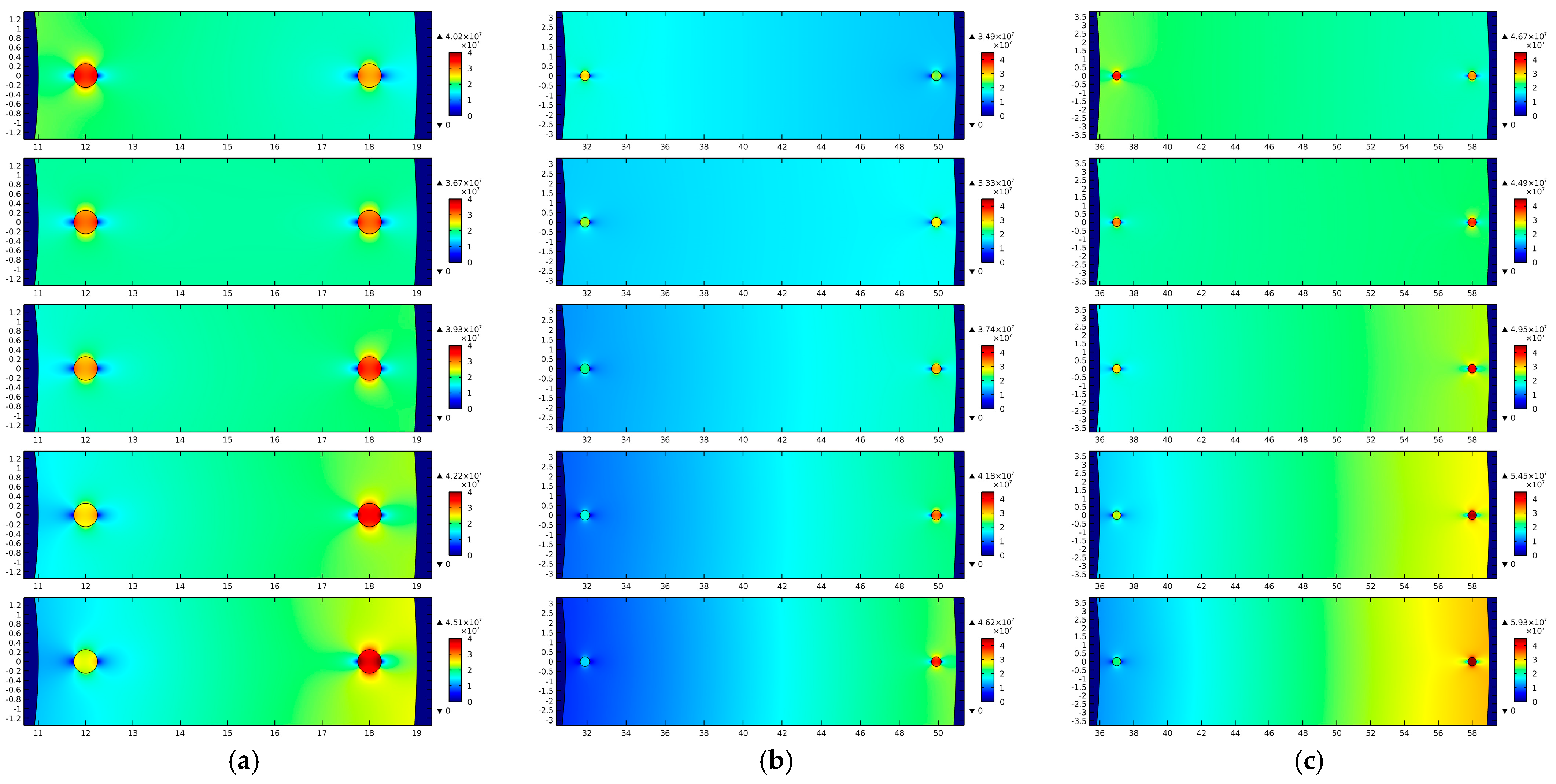
| 1st void diameter, mm | 0.5 | 0.5 | 0.5 |
| 1st void center x-coordinate, mm | 12 | 31.9 | 37 |
| 2nd void diameter, mm | 0.5 | 0.5 | 0.5 |
| 2nd void center x-coordinate, mm | 18 | 49.9 | 58 |
| Cable Core Temperature | 150 kV Cable | 320 kV Cable | 500 kV Cable | ||||||
|---|---|---|---|---|---|---|---|---|---|
| Txmin, °C | Txmax, °C | ∆T, °C | Txmin, °C | Txmax, °C | ∆T, °C | Txmin, °C | Txmax, °C | ∆T, °C | |
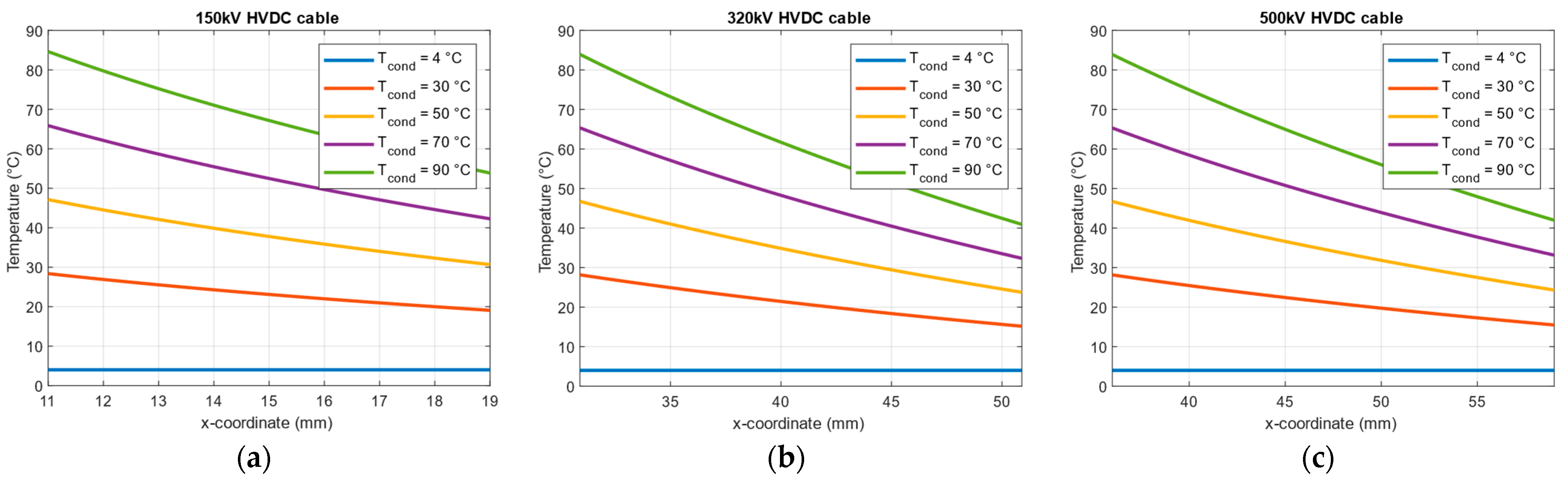
| 4 °C | 4.0 | 4.0 | 0.0 | 4.0 | 4.0 | 0.0 | 4.0 | 4.0 | 0.0 |
| 30 °C | 28.4 | 19.1 | 9.3 | 28.2 | 15.2 | 13.0 | 28.2 | 15.5 | 12.7 |
| 50 °C | 47.1 | 30.7 | 16.4 | 46.7 | 23.8 | 22.9 | 46.7 | 24.3 | 22.4 |
| 70 °C | 65.9 | 42.3 | 23.6 | 65.3 | 32.3 | 33.0 | 65.3 | 33.1 | 32.2 |
| 90 °C | 84.6 | 53.9 | 30.7 | 83.9 | 40.9 | 43.0 | 83.9 | 42.0 | 41.9 |
| Cable Core Temperature | 150 kV Cable | 320 kV Cable | 500 kV Cable | ||||||
|---|---|---|---|---|---|---|---|---|---|
| σxmin, S·m−1 | σxmax, S·m−1 | kσ, - | σxmin, S·m−1 | σxmax, S·m−1 | kσ, - | σxmin, S·m−1 | σxmax, S·m−1 | kσ, - | |
| 4 °C | 2.9 × 10⁻¹⁵ | 2.2 × 10⁻¹⁵ | 1.32 | 2.4 × 10⁻¹⁵ | 1.8 × 10⁻¹⁵ | 1.33 | 3.6 × 10⁻¹⁵ | 2.7 × 10⁻¹⁵ | 1.33 |
| 30 °C | 1.2 × 10⁻¹⁴ | 6.6 × 10⁻¹⁵ | 1.82 | 8.8 × 10⁻¹⁵ | 4.6 × 10⁻¹⁵ | 1.91 | 1.3 × 10⁻¹⁴ | 6.9 × 10⁻¹⁵ | 1.88 |
| 50 °C | 3.4 × 10⁻¹⁴ | 1.6 × 10⁻¹⁴ | 2.13 | 2.5 × 10⁻¹⁴ | 9.3 × 10⁻¹⁵ | 2.69 | 3.5 × 10⁻¹⁴ | 1.4 × 10⁻¹⁴ | 2.50 |
| 70 °C | 9.9 × 10⁻¹⁴ | 3.7 × 10⁻¹⁴ | 2.68 | 6.9 × 10⁻¹⁴ | 1.9 × 10⁻¹⁴ | 3.63 | 9.6 × 10⁻¹⁴ | 3.0 × 10⁻¹⁴ | 3.20 |
| 90 °C | 2.9 × 10⁻¹³ | 8.7 × 10⁻¹⁴ | 3.33 | 2.0 × 10⁻¹³ | 3.9 × 10⁻¹⁴ | 5.13 | 2.7 × 10⁻¹³ | 6.4 × 10⁻¹⁴ | 4.22 |
| Cable Core Temperature | 150 kV Cable | 320 kV Cable | 500 kV Cable | ||||||
|---|---|---|---|---|---|---|---|---|---|
| Exmin kV·mm−1 | Exmax kV·mm−1 | ∆E kV·mm−1 | Exmin kV·mm−1 | Exmax kV·mm−1 | ∆E kV·mm−1 | Exmin kV·mm−1 | Exmax kV·mm−1 | ∆E kV·mm−1 | |
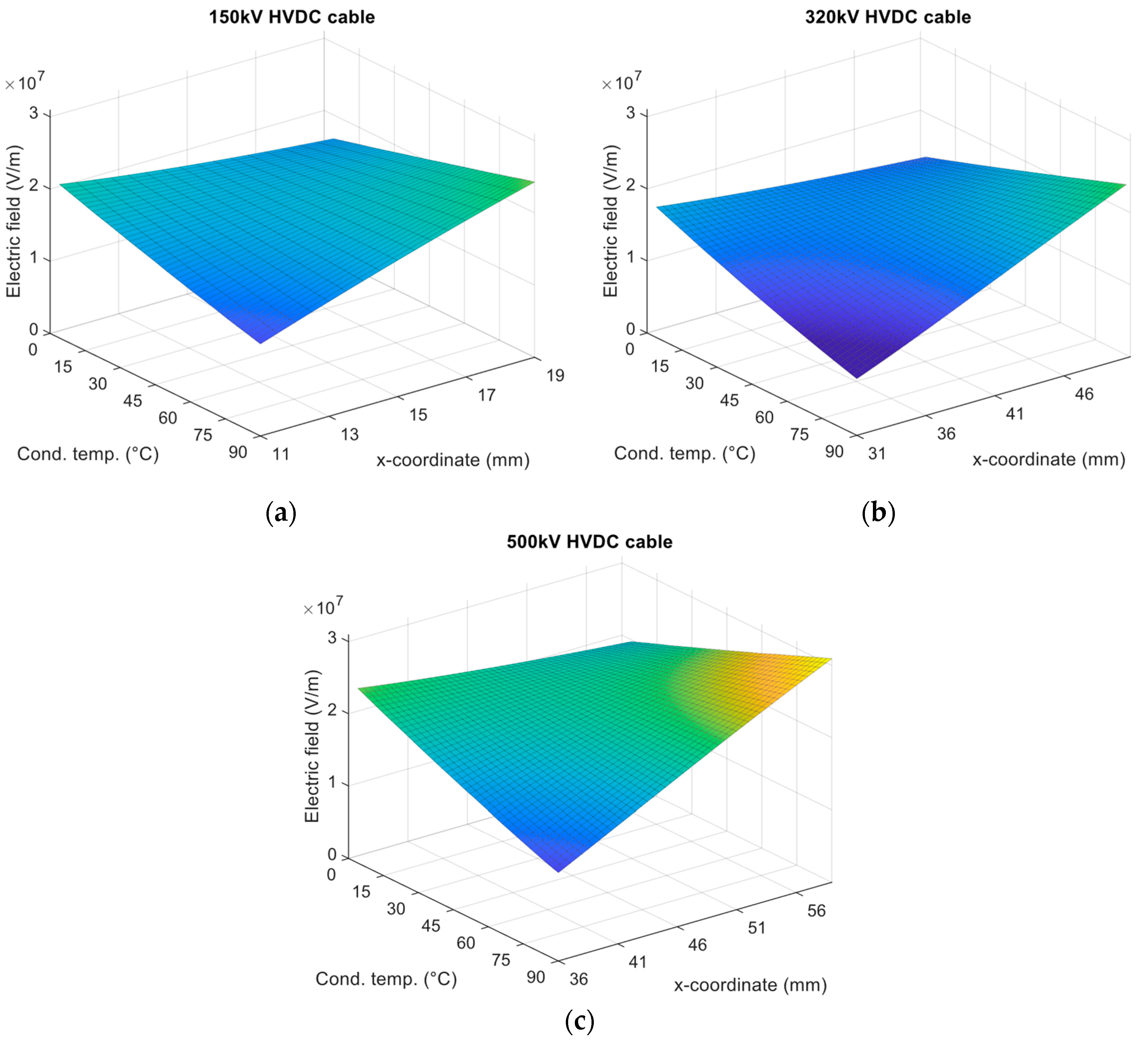
| 4 °C | 21.3 | 16.7 | 4.6 | 18.1 | 14.3 | 3.8 | 24.2 | 19.7 | 4.5 |
| 30 °C | 18.5 | 18.9 | −0.4 | 14.6 | 17.2 | −2.6 | 20.2 | 23.0 | −2.8 |
| 50 °C | 16.5 | 20.7 | −4.2 | 12.1 | 19.5 | −7.4 | 17.4 | 25.6 | −8.2 |
| 70 °C | 14.6 | 22.5 | −7.9 | 9.9 | 21.9 | −12.0 | 14.7 | 28.3 | −13.6 |
| 90 °C | 12.7 | 24.3 | −11.6 | 7.8 | 24.4 | −16.6 | 12.2 | 30.9 | −18.7 |
| Cable Core Temperature | 150 kV Cable | 320 kV Cable | 500 kV Cable | |||||||||||||||
|---|---|---|---|---|---|---|---|---|---|---|---|---|---|---|---|---|---|---|
| 1st Void | 2nd Void | 1st Void | 2nd Void | 1st Void | 2nd Void | |||||||||||||
| Evoid kV ·mm−1 | Ecable kV ·mm−1 | FEF - | Evoid kV ·mm−1 | Ecable kV ·mm−1 | FEF - | Evoid kV ·mm−1 | Ecable kV ·mm−1 | FEF - | Evoid kV ·mm−1 | Ecable kV ·mm−1 | FEF - | Evoid kV ·mm−1 | Ecable kV ·mm−1 | FEF - | Evoid kV ·mm−1 | Ecable kV ·mm−1 | FEF - | |
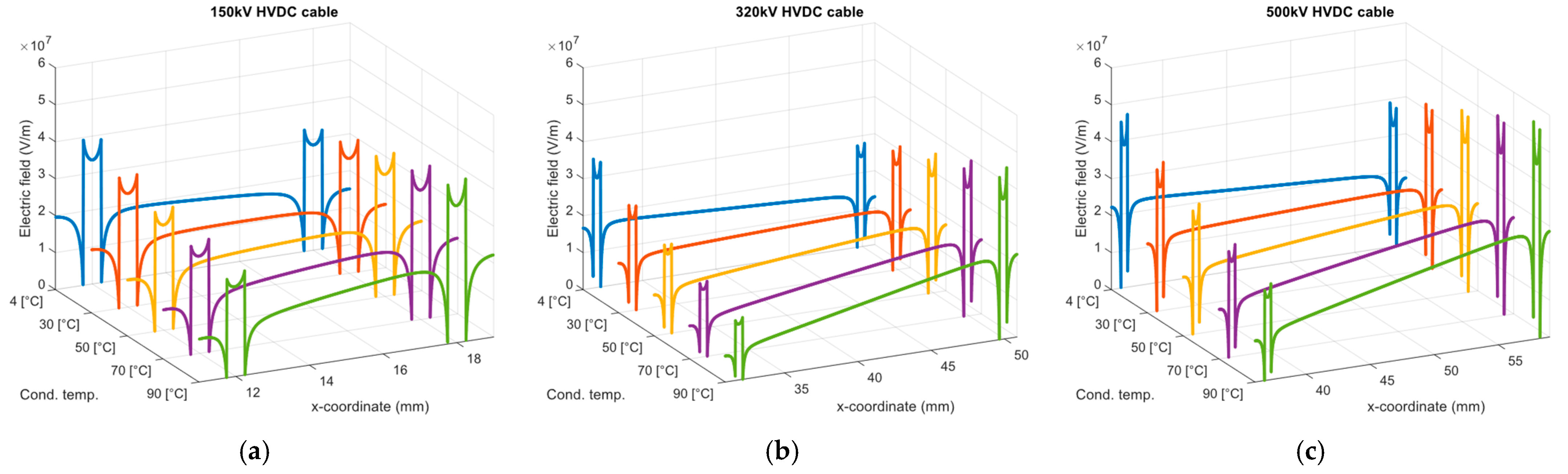
| 4 °C | 33.6 | 20.5 | 1.64 | 28.5 | 17.2 | 1.66 | 29.7 | 17.8 | 1.67 | 24.4 | 14.4 | 1.69 | 38.6 | 23.9 | 1.62 | 32.7 | 19.4 | 1.69 |
| 30 °C | 30.7 | 18.6 | 1.65 | 31.2 | 18.9 | 1.65 | 25.0 | 14.8 | 1.69 | 28.5 | 17.1 | 1.67 | 33.5 | 20.4 | 1.64 | 37.3 | 22.9 | 1.63 |
| 50 °C | 28.5 | 17.1 | 1.67 | 33.0 | 20.2 | 1.63 | 21.6 | 12.6 | 1.71 | 31.6 | 19.3 | 1.64 | 29.7 | 17.8 | 1.67 | 40.7 | 25.3 | 1.61 |
| 70 °C | 26.3 | 15.8 | 1.66 | 35.0 | 21.6 | 1.62 | 18.2 | 10.5 | 1.73 | 34.7 | 21.4 | 1.62 | 25.9 | 15.3 | 1.69 | 44.1 | 27.8 | 1.59 |
| 90 °C | 24.4 | 14.4 | 1.69 | 37.1 | 23.0 | 1.61 | 15.1 | 8.6 | 1.76 | 37.9 | 23.6 | 1.61 | 22.4 | 13.1 | 1.71 | 47.4 | 30.2 | 1.57 |
| Cable Core Temperature | 150 kV Cable | 320 kV Cable | 500 kV Cable | |||||||||
|---|---|---|---|---|---|---|---|---|---|---|---|---|
| 1st Void | 2nd Void | 1st Void | 2nd Void | 1st Void | 2nd Void | |||||||
| qav pC | ∆tav s | qav pC | ∆tav s | qav pC | ∆tav s | qav pC | ∆tav s | qav pC | ∆tav s | qav pC | ∆tav s | |
| 4 °C | 21.6 | 1072 | 21.8 | 1806 | 21.4 | 1495 | 21.9 | 2751 | 21.1 | 683 | 21.5 | 1220 |
| 30 °C | 23.1 | 343 | 22.3 | 497 | 23.1 | 577 | 22.1 | 841 | 22.8 | 265 | 21.8 | 379 |
| 50 °C | 24.3 | 155 | 23.1 | 205 | 24.4 | 280 | 22.3 | 346 | 24.1 | 120 | 22.2 | 153 |
| 70 °C | 25.5 | 67 | 23.9 | 82 | 25.9 | 162 | 22.9 | 173 | 25.4 | 64 | 22.7 | 74 |
| 90 °C | 26.5 | 26 | 24.6 | 31 | 26.8 | 73 | 23.6 | 77 | 26.5 | 32 | 23.6 | 33 |
| Insulation Zone | Unloaded Cable (‘Cold’) | Loaded Cable (‘Hot’) |
|---|---|---|
| Zone I | Insulation temperature equal to environment temperature. | High insulation temperature, the highest at the cable core. |
| Very low electrical conductivity of insulation material. | Higher electrical conductivity of the insulation material, highest near inner insulation radius. | |
| Very high electric field stress, highest near inner insulation radius (as in an AC cable). | Significant reduction of electric field stress, lowest stress near inner insulation radius. | |
| Very low repetition rate of PD pulses, but for voids with identical parameters higher than in Zone II (influence of higher E field stress). | Significantly higher repetition rate of PD pulses (several dozen times compared to a ‘cold’ cable), as a result of the combined action of higher temperature and increased E field stress. | |
| PD charges as in Zone II, with a small dispersion of values. In the case of DC voltage ripple, there is a greater variability of the PD magnitude due to the influence of lag time. | An increase in the PD magnitude (over a dozen percent), caused by an increase in Einc, due to the higher gas pressure in the closed void. | |
| Due to the higher electric field strength, PD sources of smaller critical dimension than in Zone II may be also active. | An increase in the temperature of the cable core increases the critical dimension of the void near the core. | |
| Zone II | Insulation temperature equal to environment temperature. | Increased insulation temperature, lowest on the outer radius of the insulation. |
| Very low electrical conductivity of insulation material. | Higher electrical conductivity of the insulation material, but lower than in Zone I; lowest on the outer radius of the insulation. | |
| Reduced electric field stress, lower than in Zone I, lowest near the outer radius of the insulation (as in an AC cable). | Very high electric field stress, highest near outer insulation radius. | |
| Very low repetition rate of PD pulses. | Significantly higher repetition rate of PD pulses (several dozen times compared to a ‘cold’ cable), as a result of the combined action of higher temperature and increased E field stress. | |
| PD charges as in Zone I, with a small dispersion of values. In the case of DC voltage ripple, there is a greater variability of the PD magnitude due to the influence of lag time. | A slight increase in PD magnitude (several percent), caused by an increase in Einc, due to the higher gas pressure in the closed void. | |
| Critical dimension of the gaseous void slightly larger than in Zone I. | The critical dimension of the gaseous void can be significantly smaller than in Zone I (depending on the temperature of the cable core). |
Disclaimer/Publisher’s Note: The statements, opinions and data contained in all publications are solely those of the individual author(s) and contributor(s) and not of MDPI and/or the editor(s). MDPI and/or the editor(s) disclaim responsibility for any injury to people or property resulting from any ideas, methods, instructions or products referred to in the content. |
© 2023 by the authors. Licensee MDPI, Basel, Switzerland. This article is an open access article distributed under the terms and conditions of the Creative Commons Attribution (CC BY) license (https://creativecommons.org/licenses/by/4.0/).
Share and Cite
Mikrut, P.; Zydroń, P. Numerical Modeling of PD Pulses Formation in a Gaseous Void Located in XLPE Insulation of a Loaded HVDC Cable. Energies 2023, 16, 6374. https://doi.org/10.3390/en16176374
Mikrut P, Zydroń P. Numerical Modeling of PD Pulses Formation in a Gaseous Void Located in XLPE Insulation of a Loaded HVDC Cable. Energies. 2023; 16(17):6374. https://doi.org/10.3390/en16176374
Chicago/Turabian StyleMikrut, Paweł, and Paweł Zydroń. 2023. "Numerical Modeling of PD Pulses Formation in a Gaseous Void Located in XLPE Insulation of a Loaded HVDC Cable" Energies 16, no. 17: 6374. https://doi.org/10.3390/en16176374
APA StyleMikrut, P., & Zydroń, P. (2023). Numerical Modeling of PD Pulses Formation in a Gaseous Void Located in XLPE Insulation of a Loaded HVDC Cable. Energies, 16(17), 6374. https://doi.org/10.3390/en16176374