
Optimal Allocation of Battery Energy Storage Systems to Enhance System Performance and Reliability in Unbalanced Distribution Networks


Abstract
:1. Introduction
- Reliability analysis has rarely been conducted in optimal BESS planning, particularly in unbalanced distribution systems. During the distribution system planning phase, it is significant to deliver relatively lower cost and minimal interrupted power to the customer [39].
- Almost all proposed models consider a balanced network, which is not practical. In the real world, system voltage is rarely balanced, mainly due to the unbalanced loading in the distribution system [41]. For instance, phase imbalance frequently occurs in US distribution systems, particularly the medium voltage level grid [42]. Severe voltage unbalance would magnify the system losses and shrink the capacity of the electrical components in the network [43]. Therefore, it is necessary to improve the reliability and economics of unbalanced distribution systems.
2. Reliability Assessment in the Distribution System
2.1. Expected Energy Not Supplied
2.2. Expected Interruption Cost
2.3. Total Outage Cost
2.4. Other Reliability Index
3. Problem Formulation
3.1. Objective Function
3.2. Objective Function Constraints
3.3. BESS Modelling
4. Optimization Algorithm
4.1. EGWO Approach
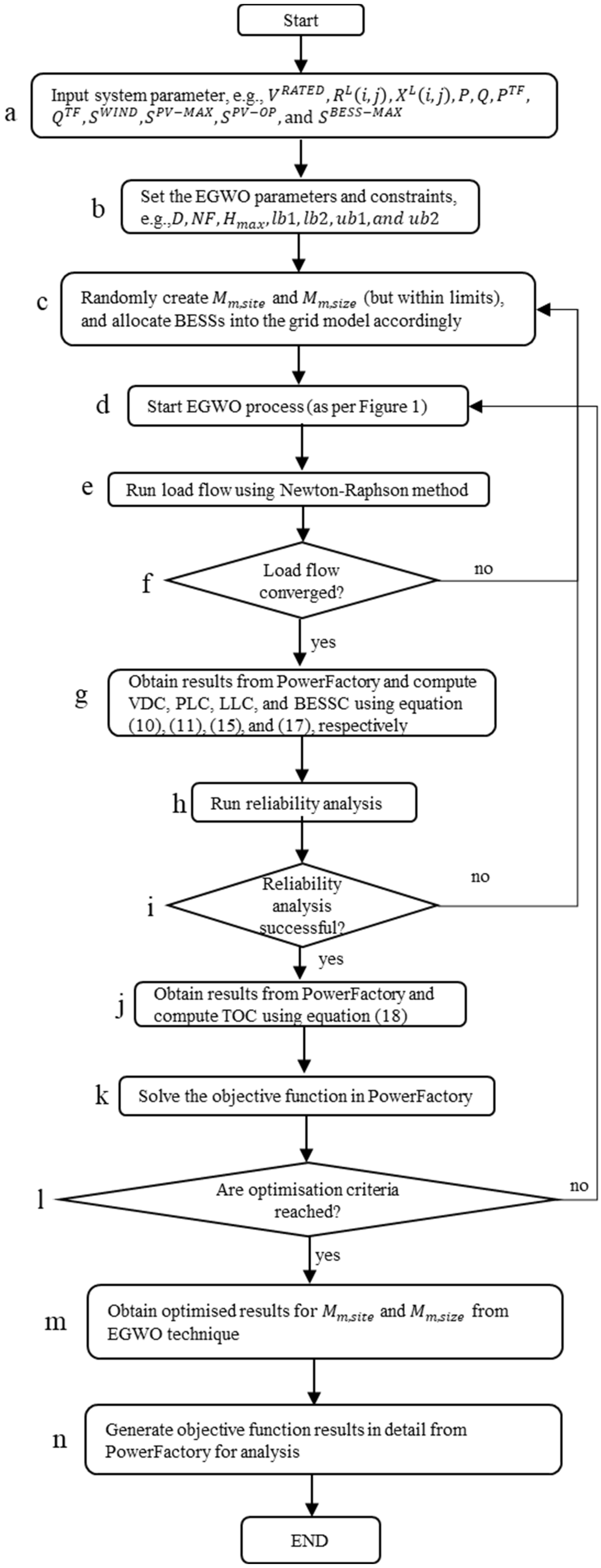
4.2. Proposed Methodology
5. Testing Network and System Performance Indices
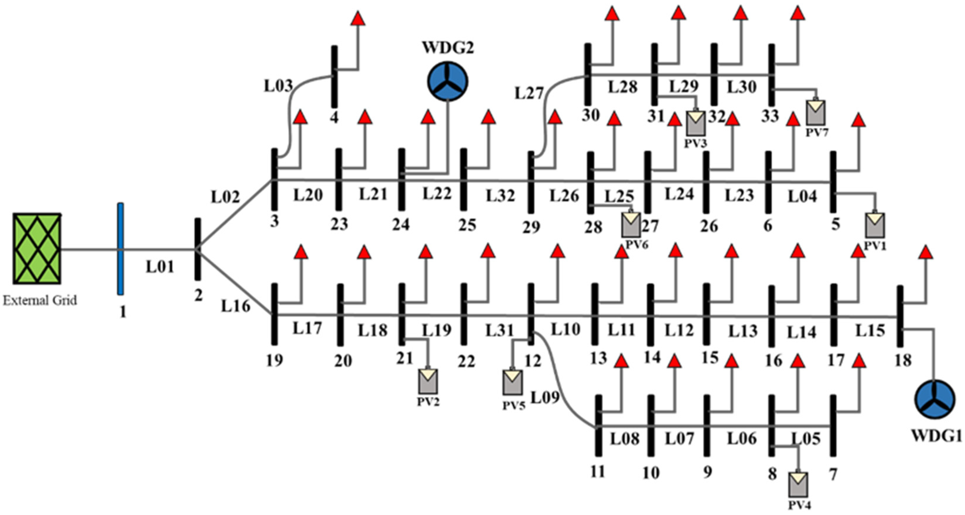
5.1. Test System
5.2. Feeder Scaling and Voltage Dependency
5.3. Indices for Evaluating System Performance Improvement
5.3.1. Indices for Voltage Deviation and Profile Improvement
5.3.2. Line Loading Index
5.3.3. Power Loss Reduction Indices
5.3.4. Reliability Indices
6. Results and Analysis
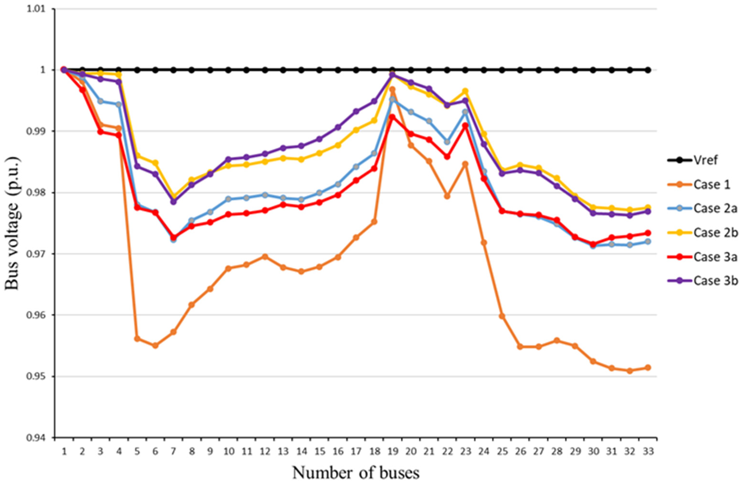
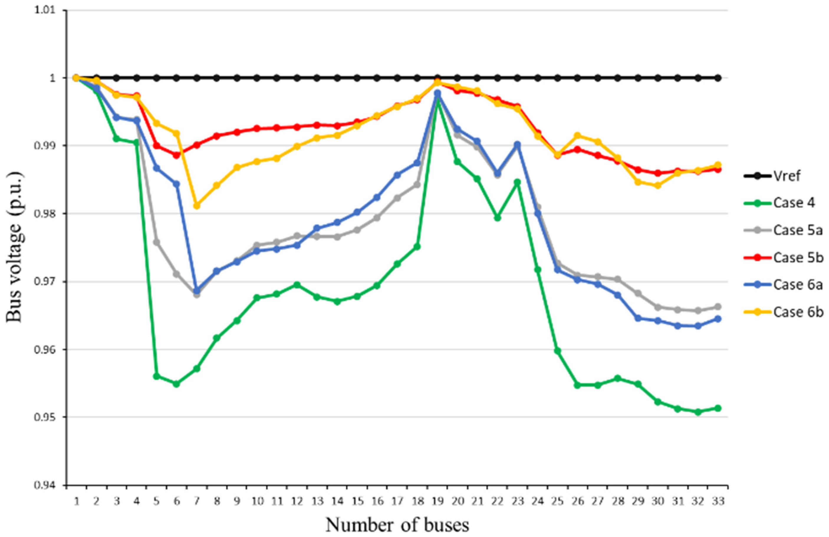
6.1. Case 1 and 4—Case without BESS Allocation in the Balanced and Unbalanced Distribution System
6.2. Case 2 and 5—Uniform BESS Allocation in the Balanced (Case 2) and Unbalanced (Case 5) Distribution System
6.3. Case 3 and 6—Non-Uniform BESS Allocation in the Balanced (Case 3) and Unbalanced Distribution System (Case 6)
6.4. Results Analysis and Comparison
6.4.1. Voltage Profile
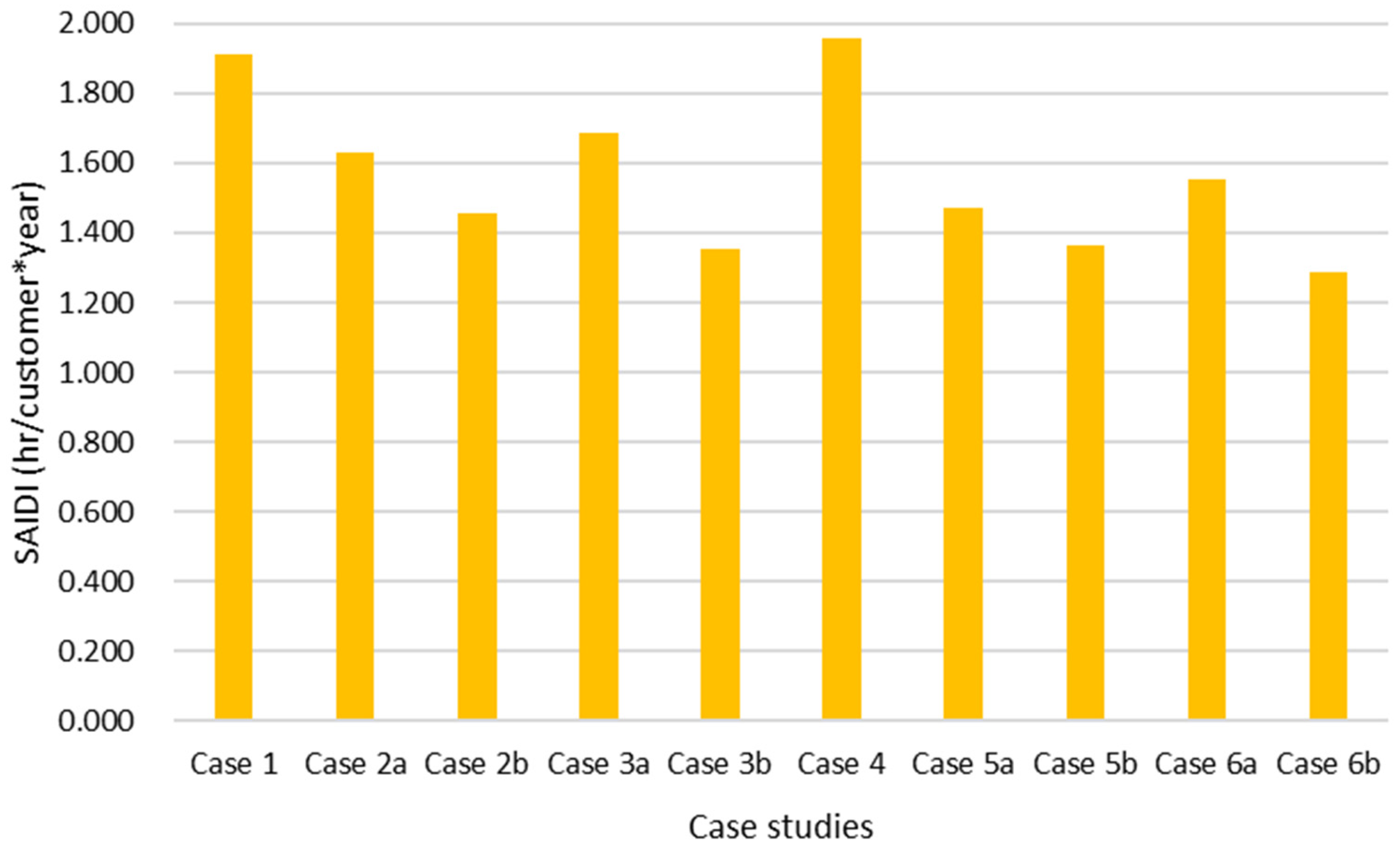
6.4.2. System Reliability Cost
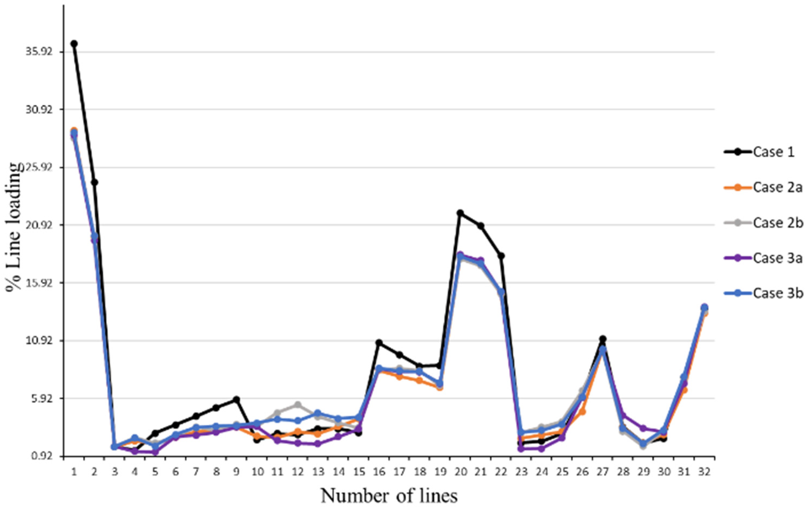
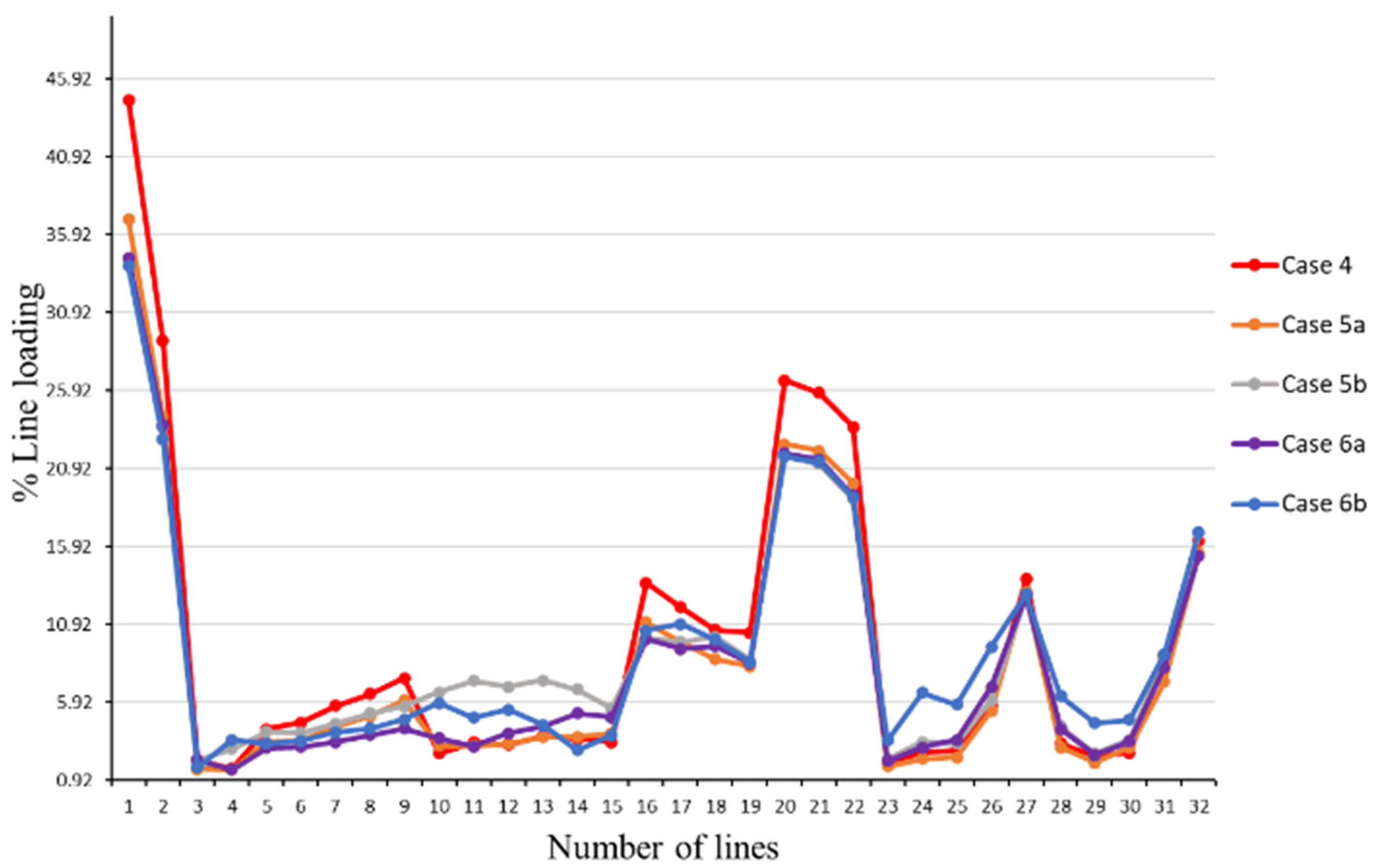
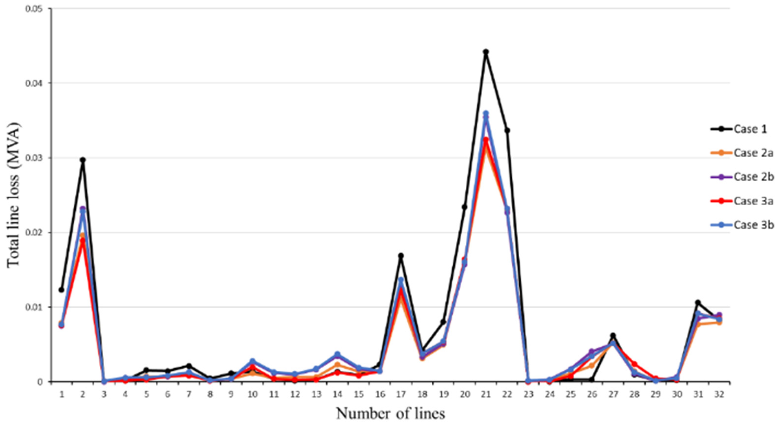
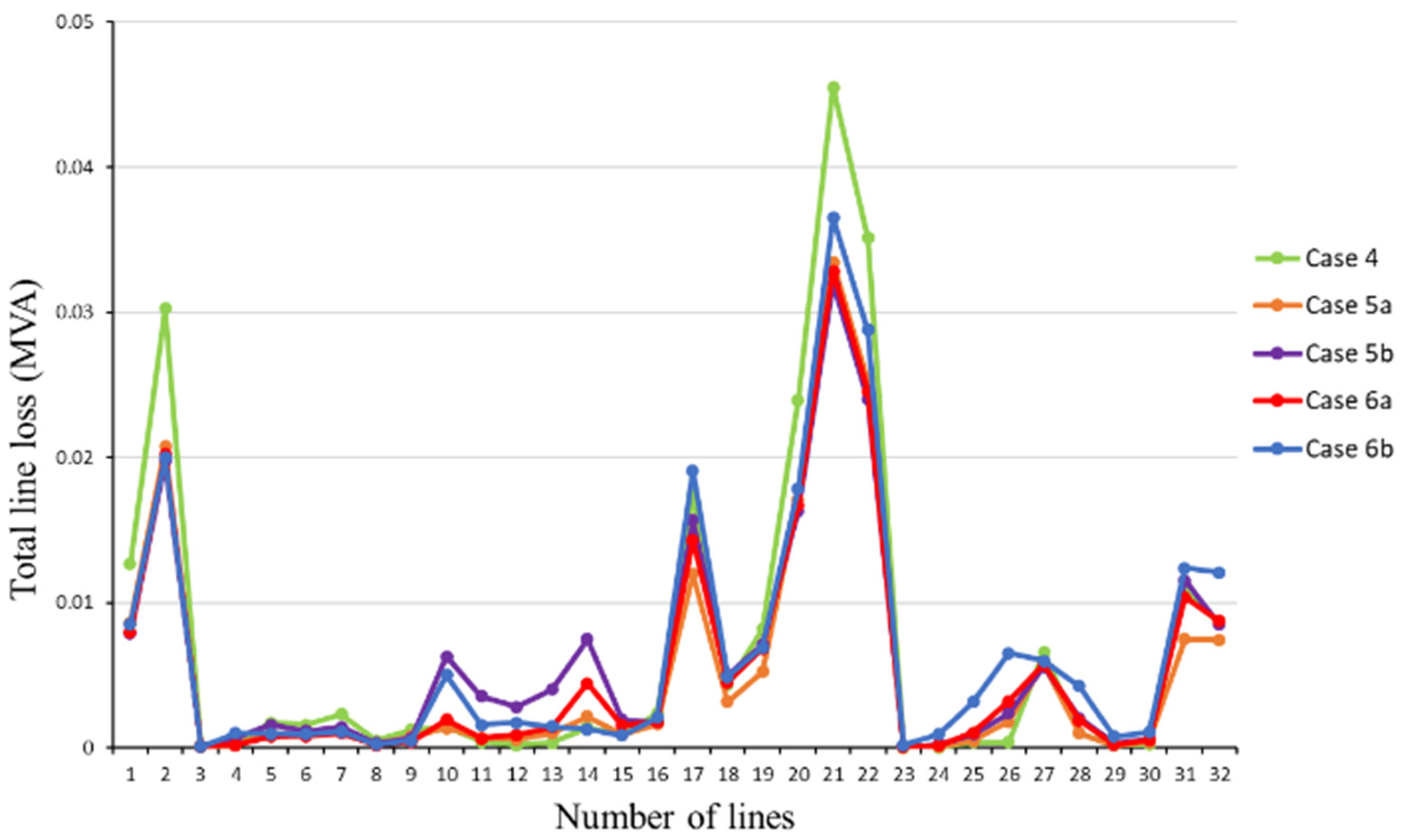
6.4.3. Line Loading and Line Losses
6.4.4. Comparison of Optimization Results with Uniform Size and Non-Uniform Size BESS
6.4.5. Comparison of Optimization Results with EGWO, GWO, and PSO Algorithms
6.5. Reliability and BESS Cost
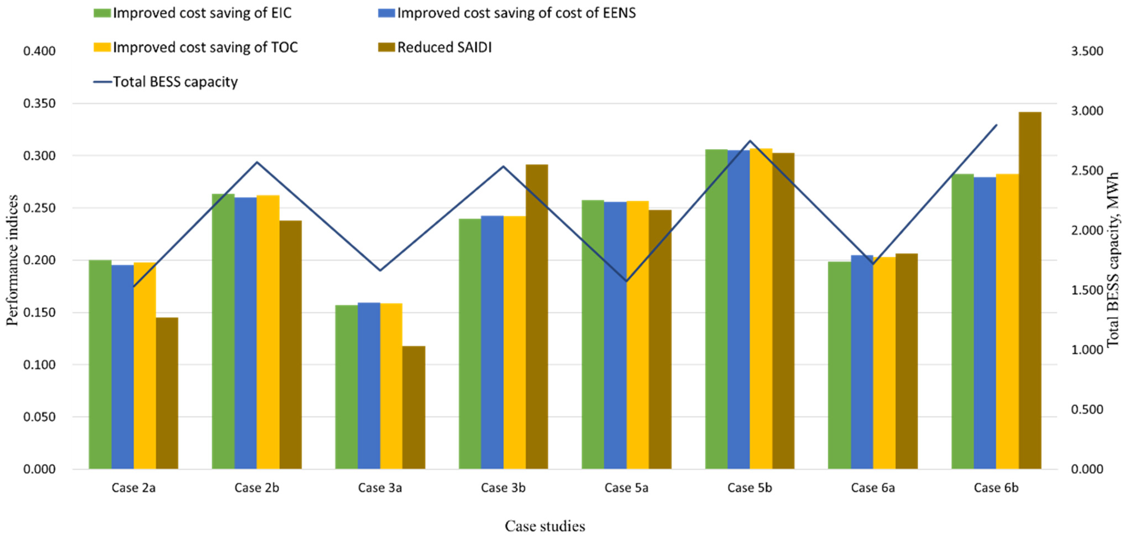
6.6. Overall Performance and BESS Cost Comparison
7. Conclusions
- A considerable reduction in TOC (19.739% and 25.673% reduction in balanced and unbalanced systems, respectively) of the wind and solar DGs penetrated distribution system is achieved with the application of BESSs, thereby improving system reliability.
- Both BESS allocation methodologies with uniform and non-uniform BESS sizes can be used to improve the system performance and economic efficiency in both balanced and unbalanced distribution systems. Nevertheless, BESS allocation with non-uniform BESS size is more regulatable in terms of system performance and economic efficiency improvement.
- The unbalanced distribution systems demand more BESS installation compared with the balanced system, leading to a larger improvement in system reliability and voltage profile; however, it also aggravates the line loading and power loss in the unbalanced system.
- A significant reduction in required iteration (18.892% on average compared with PSO, 7.905% on average compared with GWO) and computation time (18.202% on average compared with PSO, 7.637% on average compared with GWO) to reach convergency in all cases is achieved by the proposed EGWO technique. Furthermore, EGWO, GWO, and PSO approaches take more iteration (4.439% on average for EGWO, 5.79% on average for GWO, 4.474% on average for PSO) and computation time (4.907% on average for EGWO, 4.414% in average for GWO, 3.826% in average for PSO) to converge in the unbalanced system than the balanced system. Moreover, uniform BESS allocation converges faster than non-uniform BESS allocation.
Author Contributions
Funding
Institutional Review Board Statement
Informed Consent Statement
Data Availability Statement
Acknowledgments
Conflicts of Interest
Nomenclature
| time interval (h) | reactive power consumed at bus m (MVar) | ||
| BESS charging efficiency | reactive power generated at bus m (MVar) | ||
| BESS discharging efficiency | reactive power delivered from bus n to bus m (MVar) | ||
| objective function (USD) | reactive power loss of the line connecting two buses m and n (MVar) | ||
| maximum BESS energy (kWh) | input reactive power of the feeder (MVar) | ||
| minimum BESS energy (kWh) | resistance of the line connecting buses m and n | ||
| BESS energy (kWh) | maximum BESS size (MWh) | ||
| BESS energy at time t + 1 (kWh) | minimum BESS size (MWh) | ||
| BESS energy at time t (kWh) | load at bus m (p.u.) | ||
| H | iteration number | NF | number of food sources |
| e | exponential value for power computation | loading of line l after BESS placement (p.u.) | |
| total number of BESSs in service | rated ampacity of line l (p.u.) | ||
| total number of lines | state of charge of kth BESS | ||
| total number of buses | total capacity of wind DGs | ||
| BESS site info at bus m | maximum PV capacity | ||
| BESS size info at bus m | operational capacity of PV | ||
| maximum BESS power (MW) | Maximum BESS capacity | ||
| minimum BESS power (MW) | cost rate of battery unit (USD/MWh/yr) | ||
| BESS power (MW) | ub | upper boundary | |
| real power delivered from bus m to bus d (MW) | lb | lower boundary | |
| real power consumed at bus m (MW) | voltage at bus m | ||
| real power generated at bus m (MW) | bus voltage at time t | ||
| power delivered from bus n to bus m (MW) | maximum voltage limit (p.u.) | ||
| total real power loss (MW) | minimum voltage limit (p.u.) | ||
| real power loss of the line connecting bus m andn (MW) | system target voltage | ||
| BESS charging power at time t (MW) | system rated voltage (p.u.) | ||
| BESS discharging power at time t (MW) | reactance of a line connecting buses m and n | ||
| BESS power at time t (MW) | average interruption cost for load point m and contingency case x | ||
| input real power of the feeder (MW) | IEEE-RTS | IEEE reliability test system | |
| reactive power delivered from bus m to bus d (MVar) |
Appendix A. Feeder and Load Data for the Balanced and Unbalanced IEEE33-Bus Test System

| Line Number | Sending Bus | Receiving Bus | Resistance (Ω) | Reactance (Ω) | Load at Receiving Bus | |
|---|---|---|---|---|---|---|
| Real Power (kW) | Reactive Power (kVAr) | |||||
| 1 | 1 | 2 | 0.0922 | 0.0417 | 100 | 60 |
| 2 | 2 | 3 | 0.493 | 0.2511 | 90 | 40 |
| 3 | 3 | 4 | 0.366 | 0.1864 | 120 | 80 |
| 4 | 5 | 6 | 0.819 | 0.707 | 60 | 20 |
| 5 | 7 | 8 | 1.7114 | 1.2351 | 200 | 100 |
| 6 | 8 | 9 | 1.03 | 0.74 | 60 | 20 |
| 7 | 9 | 10 | 1.04 | 0.74 | 60 | 20 |
| 8 | 10 | 11 | 0.1966 | 0.065 | 45 | 30 |
| 9 | 11 | 12 | 0.3744 | 0.1238 | 60 | 35 |
| 10 | 12 | 13 | 14.68 | 1.155 | 60 | 35 |
| 11 | 13 | 14 | 0.5416 | 0.7129 | 120 | 80 |
| 12 | 14 | 15 | 0.591 | 0.526 | 60 | 10 |
| 13 | 15 | 16 | 0.7463 | 0.545 | 60 | 20 |
| 14 | 16 | 17 | 1.289 | 1.721 | 60 | 20 |
| 15 | 17 | 18 | 0.732 | 0.574 | 90 | 40 |
| 16 | 2 | 19 | 0.164 | 0.1565 | 90 | 40 |
| 17 | 19 | 20 | 1.5042 | 1.3154 | 90 | 40 |
| 18 | 20 | 21 | 0.4095 | 0.4784 | 90 | 40 |
| 19 | 21 | 22 | 0.7089 | 0.9373 | 90 | 40 |
| 20 | 3 | 23 | 0.4512 | 0.3083 | 90 | 50 |
| 21 | 23 | 24 | 0.898 | 0.7091 | 420 | 200 |
| 22 | 24 | 25 | 0.896 | 0.7011 | 420 | 200 |
| 23 | 6 | 26 | 0.203 | 0.1034 | 60 | 25 |
| 24 | 26 | 27 | 0.2842 | 0.1447 | 60 | 25 |
| 25 | 27 | 28 | 1.059 | 0.9337 | 60 | 20 |
| 26 | 28 | 29 | 0.8042 | 0.7006 | 120 | 70 |
| 27 | 29 | 30 | 0.5075 | 0.2585 | 200 | 600 |
| 28 | 30 | 31 | 0.9744 | 0.963 | 150 | 70 |
| 29 | 31 | 32 | 0.3105 | 0.3619 | 210 | 100 |
| 30 | 32 | 33 | 0.341 | 0.5302 | 60 | 40 |
| 31 * | 12 | 22 | 0 | 2 | 90 | 40 |
| 32 * | 25 | 29 | 0 | 0.5 | 120 | 70 |
| Bus# | Phase A | Phase B | Phase C | |||
|---|---|---|---|---|---|---|
| P Load (kW) | Q Load (kVAr) | P Load (kW) | Q Load (kVAr) | P Load (kW) | Q Load (kVAr) | |
| 1 | 0 | 0 | 0 | 0 | 0 | 0 |
| 2 | 45.38364 | 27.20091 | 46.97678 | 28.15615 | 7.651557 | 4.586019 |
| 3 | 40.39426 | 17.96903 | 41.40079 | 18.41674 | 8.280372 | 3.683133 |
| 4 | 49.86655 | 33.22193 | 24.70916 | 16.46191 | 45.47072 | 30.29369 |
| 5 | 20.16107 | 10.0808 | 13.36378 | 6.68189 | 26.41769 | 13.20885 |
| 6 | 26.5972 | 8.889419 | 28.53333 | 9.536398 | 4.813076 | 1.608633 |
| 7 | 44.63782 | 22.31891 | 92.25998 | 46.12999 | 63.12615 | 31.56307 |
| 8 | 59.19779 | 29.59916 | 58.84519 | 29.42233 | 81.98097 | 40.99049 |
| 9 | 15.41424 | 5.151792 | 27.3318 | 9.135175 | 17.19704 | 5.747483 |
| 10 | 24.80639 | 8.291057 | 18.93923 | 6.329818 | 16.19692 | 5.413576 |
| 11 | 18.15976 | 12.08478 | 21.68315 | 14.42961 | 5.194532 | 3.457145 |
| 12 | 13.46956 | 7.851367 | 14.87785 | 8.671978 | 31.59566 | 18.41674 |
| 13 | 22.79707 | 13.28792 | 26.14736 | 15.24114 | 10.99865 | 6.411024 |
| 14 | 54.15552 | 36.07964 | 35.9386 | 23.94304 | 29.95177 | 19.95485 |
| 15 | 12.29795 | 2.038706 | 11.59487 | 1.922239 | 36.05026 | 5.976143 |
| 16 | 17.19276 | 5.746415 | 26.55286 | 8.87446 | 16.19692 | 5.413576 |
| 17 | 14.27842 | 4.772473 | 25.79636 | 8.621759 | 19.8683 | 6.640218 |
| 18 | 34.66922 | 15.42225 | 15.7973 | 7.027551 | 39.60784 | 17.6191 |
| 19 | 38.60558 | 17.173 | 42.71238 | 19.00014 | 8.756925 | 3.895766 |
| 20 | 29.79417 | 13.25372 | 40.05341 | 17.8173 | 20.22732 | 8.997872 |
| 21 | 18.95633 | 8.432634 | 37.82504 | 16.82627 | 33.29352 | 14.81053 |
| 22 | 42.80748 | 19.04234 | 40.01441 | 17.80021 | 7.252471 | 3.226348 |
| 23 | 22.80081 | 12.65803 | 21.40855 | 11.88497 | 45.86553 | 25.46245 |
| 24 | 143.0973 | 68.16254 | 125.6069 | 59.83088 | 151.2179 | 72.03053 |
| 25 | 137.0501 | 65.28186 | 209.1078 | 99.60541 | 73.76417 | 35.13669 |
| 26 | 22.06835 | 9.205162 | 28.87098 | 12.04257 | 9.003749 | 3.755792 |
| 27 | 19.7903 | 8.254728 | 18.74103 | 7.817175 | 21.41175 | 8.931091 |
| 28 | 25.42879 | 8.498881 | 24.85768 | 8.308153 | 9.656605 | 3.227416 |
| 29 | 37.73101 | 22.01385 | 22.12872 | 12.91073 | 60.18723 | 35.11585 |
| 30 | 39.19273 | 117.5782 | 86.54295 | 259.6283 | 74.28828 | 222.8654 |
| 31 | 57.7863 | 26.97919 | 26.62017 | 12.4283 | 65.61202 | 30.63294 |
| 32 | 73.98108 | 35.2398 | 85.37026 | 40.66513 | 50.60969 | 24.10705 |
| 33 | 12.19644 | 8.152686 | 14.31956 | 9.571659 | 33.42708 | 22.34456 |
Appendix B. PSO Technique
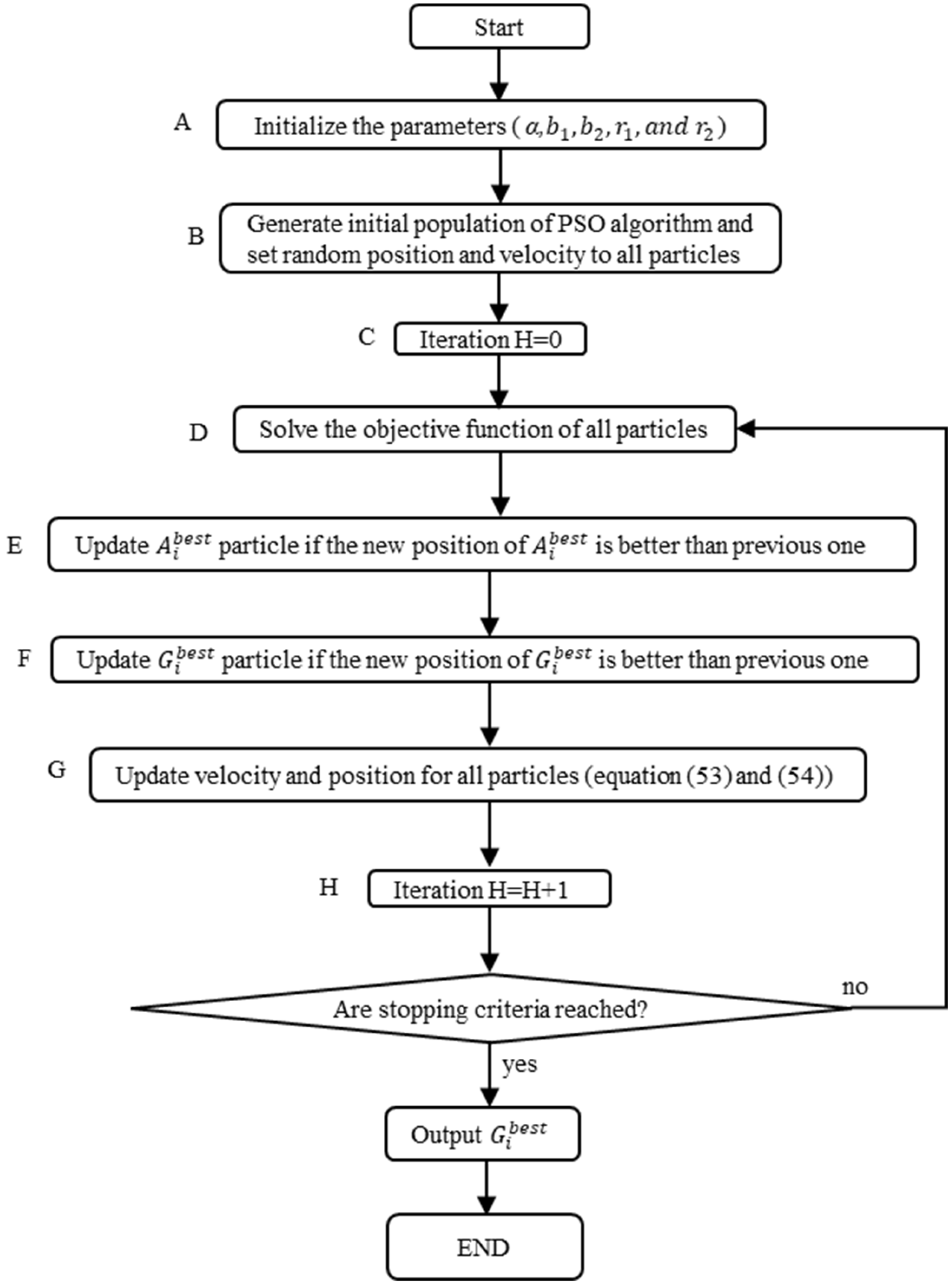
| Type | Parameters/Variables | Description/Settings |
|---|---|---|
| Input parameters | Critical for the distribution system model | |
| Output parameters | , , , , and | Critical for the objective function |
| Decision variables | Determine the sizes of BESSs in MVA with a unity power factor. | |
| Determine the locations of BESSs in the grid. | ||
| PSO parameters | Settings: | |
| PSO bounds | Settings: lb1 = 0.1 MVA and ub1 = 2 MVA Settings: lb2 = 0 and ub2 = 1 |
References
- Zhang, D.; Shafiullah, G.; Das, C.K.; Wong, K.W. A systematic review of optimal planning and deployment of distributed generation and energy storage systems in power networks. J. Energy Storage 2022, 56, 105937. [Google Scholar] [CrossRef]
- Shafiullah, G. Hybrid renewable energy integration (HREI) system for subtropical climate in Central Queensland, Australia. Renew. Energy 2016, 96, 1034–1053. [Google Scholar] [CrossRef]
- Goel, L. Power system reliability cost/benefit assessment and application in perspective. Comput. Electr. Eng. 1998, 24, 315–324. [Google Scholar] [CrossRef]
- International Energy Agency. Renewable Electricity Growth is Accelerating Faster than Ever Worldwide, Supporting the Emergence of the New Global Energy Economy. 1 December 2021. Available online: https://www.iea.org/news/renewable-electricity-growth-is-accelerating-faster-than-ever-worldwide-supporting-the-emergence-of-the-new-global-energy-economy (accessed on 13 May 2023).
- Billinton, R.; Allan, R.N. Reliability Evaluation of Engineering Systems; Springer: Berlin/Heidelberg, Germany, 1992; Volume 792. [Google Scholar]
- Li, W. Reliability Assessment of Electric Power Systems Using Monte Carlo Methods; Springer Science & Business Media: Berlin/Heidelberg, Germany, 2013. [Google Scholar]
- Adefarati, T.; Bansal, R. Reliability and economic assessment of a microgrid power system with the integration of renewable energy resources. Appl. Energy 2017, 206, 911–933. [Google Scholar] [CrossRef]
- Zhang, C.; Zhao, T.; Xu, Q.; An, L.; Zhao, G. Effects of operating temperature on the performance of vanadium redox flow batteries. Appl. Energy 2015, 155, 349–353. [Google Scholar] [CrossRef]
- Rana, M.M.; Uddin, M.; Sarkar, M.R.; Shafiullah, G.; Mo, H.; Atef, M. A review on hybrid photovoltaic–Battery energy storage system: Current status, challenges, and future directions. J. Energy Storage 2022, 51, 104597. [Google Scholar] [CrossRef]
- Zhou, P.; Jin, R.Y.; Fan, L.W. Reliability and economic evaluation of power system with renewables: A review. Renew. Sustain. Energy Rev. 2016, 58, 537–547. [Google Scholar] [CrossRef]
- Shafiullah, G.M.; Arif, M.T.; Oo, A.M.T. Mitigation strategies to minimize potential technical challenges of renewable energy integration. Sustain. Energy Technol. Assess. 2018, 25, 24–42. [Google Scholar] [CrossRef]
- Babacan, O.; Torre, W.; Kleissl, J. Siting and sizing of distributed energy storage to mitigate voltage impact by solar PV in distribution systems. Sol. Energy 2017, 146, 199–208. [Google Scholar] [CrossRef]
- Das, C.K.; Bass, O.; Mahmoud, T.S.; Kothapalli, G.; Mousavi, N.; Habibi, D.; Masoum, M.A. Optimal allocation of distributed energy storage systems to improve performance and power quality of distribution networks. Appl. Energy 2019, 252, 113468. [Google Scholar] [CrossRef]
- Das, C.K.; Bass, O.; Kothapalli, G.; Mahmoud, T.S.; Habibi, D. Optimal placement of distributed energy storage systems in distribution networks using artificial bee colony algorithm. Appl. Energy 2018, 232, 212–228. [Google Scholar] [CrossRef]
- Kalkhambkar, V.; Kumar, R.; Bhakar, R. Methodology for joint allocation of energy storage and renewable distributed generation. In Proceedings of the 2016 International Conference on Recent Advances and Innovations in Engineering (ICRAIE), Jaipur, India, 23–25 December 2016; pp. 1–8. [Google Scholar]
- Lei, J.; Gong, Q. Operating strategy and optimal allocation of large-scale VRB energy storage system in active distribution networks for solar/wind power applications. IET Gener. Transm. Distrib. 2017, 11, 2403–2411. [Google Scholar] [CrossRef]
- Nick, M.; Cherkaoui, R.; Paolone, M. Optimal planning of distributed energy storage systems in active distribution networks embedding grid reconfiguration. IEEE Trans. Power Syst. 2017, 33, 1577–1590. [Google Scholar] [CrossRef]
- Mehmood, K.K.; Khan, S.U.; Lee, S.-J.; Haider, Z.M.; Rafique, M.K.; Kim, C.-H. Optimal sizing and allocation of battery energy storage systems with wind and solar power DGs in a distribution network for voltage regulation considering the lifespan of batteries. IET Renew. Power Gener. 2017, 11, 1305–1315. [Google Scholar] [CrossRef]
- Taskforce, E.T. DER Roadmap. December 2019; p. 77. Available online: https://www.wa.gov.au/system/files/2020-04/DER_Roadmap.pdf (accessed on 15 June 2023).
- Yang, M.; Chen, C.; Que, B.; Zhou, Z.; Yang, Q. Optimal placement and configuration of hybrid energy storage system in power distribution networks with distributed photovoltaic sources. In Proceedings of the 2018 2nd IEEE Conference on Energy Internet and Energy System Integration (EI2), Beijing, China, 20–22 October 2018; pp. 1–6. [Google Scholar]
- Yan, N.; Zhang, B.; Li, W.; Ma, S. Hybrid energy storage capacity allocation method for active distribution network considering demand side response. IEEE Trans. Appl. Supercond. 2018, 29, 1–4. [Google Scholar] [CrossRef]
- Awad, A.S.; El-Fouly, T.H.; Salama, M.M. Optimal ESS allocation and load shedding for improving distribution system reliability. IEEE Trans. Smart Grid 2014, 5, 2339–2349. [Google Scholar] [CrossRef]
- Saboori, H.; Hemmati, R.; Jirdehi, M.A. Reliability improvement in radial electrical distribution network by optimal planning of energy storage systems. Energy 2015, 93, 2299–2312. [Google Scholar] [CrossRef]
- Moradijoz, M.; Moghaddam, M.P.; Haghifam, M. A flexible active distribution system expansion planning model: A risk-based approach. Energy 2018, 145, 442–457. [Google Scholar] [CrossRef]
- Murali, G.; Manivannan, A. Analysis of power quality problems in solar power distribution system. Int. J. Eng. Res. Appl. 2013, 3, 799–805. [Google Scholar]
- Abdeltawab, H.; Mohamed, Y.A.-R.I. Mobile Energy Storage Sizing and Allocation for Multi-Services in Power Distribution Systems. IEEE Access 2019, 7, 176613–176623. [Google Scholar] [CrossRef]
- Lei, J.; Gong, Q.; Liu, J.; Qiao, H.; Wang, B. Optimal allocation of a VRB energy storage system for wind power applications considering the dynamic efficiency and life of VRB in active distribution networks. IET Renew. Power Gener. 2019, 13, 563–571. [Google Scholar] [CrossRef]
- Li, W.; Lu, C.; Pan, X.; Song, J. Optimal placement and capacity allocation of distributed energy storage devices in distribution networks. In Proceedings of the 2017 13th IEEE Conference on Automation Science and Engineering (CASE), Xi’an, China, 20–23 August 2017; pp. 1403–1407. [Google Scholar]
- Wang, S.; Wang, K.; Teng, F.; Strbac, G.; Wu, L. Optimal allocation of ESSs for mitigating fluctuation in active distribution network. Energy Procedia 2017, 142, 3572–3577. [Google Scholar] [CrossRef]
- Kim, I. Optimal capacity of storage systems and photovoltaic systems able to control reactive power using the sensitivity analysis method. Energy 2018, 150, 642–652. [Google Scholar] [CrossRef]
- Ghatak, S.R.; Sannigrahi, S.; Acharjee, P. Multi-objective approach for strategic incorporation of solar energy source, battery storage system, and DSTATCOM in a smart grid environment. IEEE Syst. J. 2018, 13, 3038–3049. [Google Scholar] [CrossRef]
- Li, B.; Li, X.; Bai, X.; Li, Z. Storage capacity allocation strategy for distribution network with distributed photovoltaic generators. J. Mod. Power Syst. Clean Energy 2018, 6, 1234–1243. [Google Scholar] [CrossRef]
- Ahmed, H.M.; Awad, A.S.; Ahmed, M.H.; Salama, M. Mitigating voltage-sag and voltage-deviation problems in distribution networks using battery energy storage systems. Electr. Power Syst. Res. 2020, 184, 106294. [Google Scholar] [CrossRef]
- Carpinelli, G.; Mottola, F.; Noce, C.; Russo, A.; Varilone, P. A new hybrid approach using the simultaneous perturbation stochastic approximation method for the optimal allocation of electrical energy storage systems. Energies 2018, 11, 1505. [Google Scholar] [CrossRef]
- Wen, S.; Lan, H.; Fu, Q.; Yu, D.C.; Hong, Y.-Y.; Cheng, P. Optimal allocation of energy storage system considering multi-correlated wind farms. Energies 2017, 10, 625. [Google Scholar] [CrossRef]
- Aming, D.; Rajapakse, A.; Molinski, T.; Innes, E. A technique for evaluating the reliability improvement due to energy storage systems. In Proceedings of the 2007 Canadian Conference on Electrical and Computer Engineering, Vancouver, BC, Canada, 22–26 April 2007; pp. 413–416. [Google Scholar]
- Zhang, D.; Das, C.K.; Shafiullah, G.; Wong, K.W. Optimal allocation of distributed energy storage systems in unbalanced distribution networks. In Proceedings of the 2021 IEEE Asia-Pacific Conference on Computer Science and Data Engineering (CSDE), Brisbane, Australia, 8–10 December 2021; pp. 1–6. [Google Scholar]
- Wang, S.; Luo, F.; Dong, Z.Y.; Ranzi, G. Joint planning of active distribution networks considering renewable power uncertainty. Int. J. Electr. Power Energy Syst. 2019, 110, 696–704. [Google Scholar] [CrossRef]
- Ghiasi, M.; Ghadimi, N.; Ahmadinia, E. An analytical methodology for reliability assessment and failure analysis in distributed power system. SN Appl. Sci. 2019, 1, 44. [Google Scholar] [CrossRef]
- Shoeb, M.A.; Shahnia, F.; Shafiullah, G. A multilayer and event-triggered voltage and frequency management technique for microgrid’s central controller considering operational and sustainability aspects. IEEE Trans. Smart Grid 2018, 10, 5136–5151. [Google Scholar] [CrossRef]
- Albadi, M.H.; Al Hinai, A.S.; Al-Badi, A.H.; Al Riyami, M.S.; Al Hinai, S.M.; Al Abri, R.S. Unbalance in power systems: Case study. In Proceedings of the 2015 IEEE International Conference on Industrial Technology (ICIT), Seville, Spain, 17–19 March 2015; pp. 1407–1411. [Google Scholar]
- Ma, K.; Fang, L.; Kong, W. Review of distribution network phase unbalance: Scale, causes, consequences, solutions, and future research directions. CSEE J. Power Energy Syst. 2020, 6, 479–488. [Google Scholar]
- Meersman, B.; Renders, B.; Degroote, L.; Vandoorn, T.; Vandevelde, L. Three-phase inverter-connected DG-units and voltage unbalance. Electr. Power Syst. Res. 2011, 81, 899–906. [Google Scholar] [CrossRef]
- Das, C.K.; Bass, O.; Mahmoud, T.S.; Kothapalli, G.; Masoum, M.A.; Mousavi, N. An optimal allocation and sizing strategy of distributed energy storage systems to improve performance of distribution networks. J. Energy Storage 2019, 26, 100847. [Google Scholar] [CrossRef]
- Mohsen, M.; Youssef, A.-R.; Ebeed, M.; Kamel, S. Optimal planning of renewable distributed generation in distribution systems using grey wolf optimizer GWO. In Proceedings of the 2017 Nineteenth International Middle East Power Systems Conference (MEPCON), Cairo, Egypt, 19–21 December 2017; pp. 915–921. [Google Scholar]
- Ansari, M.M.; Guo, C.; Shaikh, M.S.; Chopra, N.; Haq, I.; Shen, L. Planning for distribution system with grey wolf optimization method. J. Electr. Eng. Technol. 2020, 15, 1485–1499. [Google Scholar] [CrossRef]
- Goli, P.; Yelem, S.; Muaddi, S.; Gampa, S.R.; Shireen, W. Optimal Planning of Smart Charging Facilities using Grey Wolf Optimizer. In Proceedings of the 2022 IEEE Texas Power and Energy Conference (TPEC), College Station, TX, USA, 28 February–1 March 2022; pp. 1–6. [Google Scholar]
- Sultana, U.; Khairuddin, A.B.; Mokhtar, A.; Zareen, N.; Sultana, B. Grey wolf optimizer based placement and sizing of multiple distributed generation in the distribution system. Energy 2016, 111, 525–536. [Google Scholar] [CrossRef]
- Ikeda, S.; Ooka, R. Metaheuristic optimization methods for a comprehensive operating schedule of battery, thermal energy storage, and heat source in a building energy system. Appl. Energy 2015, 151, 192–205. [Google Scholar] [CrossRef]
- Koad, R.B.; Zobaa, A.F.; El-Shahat, A. A novel MPPT algorithm based on particle swarm optimization for photovoltaic systems. IEEE Trans. Sustain. Energy 2016, 8, 468–476. [Google Scholar] [CrossRef]
- Allan, R.N.; Billinton, R.; Sjarief, I.; Goel, L.; So, K. A reliability test system for educational purposes-basic distribution system data and results. IEEE Trans. Power Syst. 1991, 6, 813–820. [Google Scholar] [CrossRef]
- Billinton, R.; Allan, R.N. Reliability Evaluation of Power Systems; Springer Science & Business Media: Berlin/Heidelberg, Germany, 2013. [Google Scholar]
- Adefarati, T.; Bansal, R. Integration of renewable distributed generators into the distribution system: A review. IET Renew. Power Gener. 2016, 10, 873–884. [Google Scholar] [CrossRef]
- Adefarati, T.; Bansal, R. Reliability assessment of distribution system with the integration of renewable distributed generation. Appl. Energy 2017, 185, 158–171. [Google Scholar] [CrossRef]
- Nojavan, S.; Zare, K. Demand Response Application in Smart Grid; Springer: Berlin/Heidelberg, Germany, 2020. [Google Scholar]
- IEEE Guide for Electric Power Distribution Reliability Indices; IEEE: Piscataway, NJ, USA, 2012; pp. 1–43.
- Jayasekara, N.; Masoum, M.A.; Wolfs, P.J. Optimal operation of distributed energy storage systems to improve distribution network load and generation hosting capability. IEEE Trans. Sustain. Energy 2015, 7, 250–261. [Google Scholar] [CrossRef]
- Zhong, S.; Qiu, J.; Sun, L.; Liu, Y.; Zhang, C.; Wang, G. Coordinated planning of distributed WT, shared BESS and individual VESS using a two-stage approach. Int. J. Electr. Power Energy Syst. 2020, 114, 105380. [Google Scholar] [CrossRef]
- Bloomberg Finance. Behind the Scenes Take on Lithium-ion Battery Prices. 2019. Available online: https://about.bnef.com/blog/behind-scenes-take-lithium-ion-battery-prices (accessed on 22 June 2023).
- Valøen, L.O.; Shoesmith, M.I. The effect of PHEV and HEV duty cycles on battery and battery pack performance. In Proceedings of the PHEV 2007 Conference, Winnipeg, MB, Canada, 1–2 November 2007; pp. 4–5. [Google Scholar]
- Frankel, D.; Kane, S.; Tryggestad, C. The New Rules of Competition in Energy Storage. 2018. Available online: https://www.mckinsey.com/ (accessed on 20 June 2023).
- Asenbauer, J.; Eisenmann, T.; Kuenzel, M.; Kazzazi, A.; Chen, Z.; Bresser, D. The success story of graphite as a lithium-ion anode material–fundamentals, remaining challenges, and recent developments including silicon (oxide) composites. Sustain. Energy Fuels 2020, 4, 5387–5416. [Google Scholar] [CrossRef]
- Hornsdale Power Reserve. Available online: https://hornsdalepowerreserve.com.au/?sfw=pass1619474757 (accessed on 18 June 2023).
- Jabr, R.A.; Džafić, I.; Pal, B.C. Robust optimization of storage investment on transmission networks. IEEE Trans. Power Syst. 2014, 30, 531–539. [Google Scholar] [CrossRef]
- Luo, K. Enhanced grey wolf optimizer with a model for dynamically estimating the location of the prey. Appl. Soft Comput. 2019, 77, 225–235. [Google Scholar] [CrossRef]
- Mirjalili, S.; Mirjalili, S.M.; Lewis, A. Grey wolf optimizer. Adv. Eng. Softw. 2014, 69, 46–61. [Google Scholar] [CrossRef]
- Baran, M.E.; Wu, F.F. Network reconfiguration in distribution systems for loss reduction and load balancing. IEEE Trans. Power Deliv. 1989, 4, 1401–1407. [Google Scholar] [CrossRef]
- Swarnkar, A.; Gupta, N.; Niazi, K.R. Adapted ant colony optimization for efficient reconfiguration of balanced and unbalanced distribution systems for loss minimization. Swarm Evol. Comput. 2011, 1, 129–137. [Google Scholar] [CrossRef]
- Power, W. Technical Rules December. 2016. Available online: https://www.westernpower.com.au/media/2312/technical-rules-20161201.pdf (accessed on 16 June 2023).
- Sereeter, B.; Vuik, K.; Witteveen, C. Newton Power Flow Methods for Unbalanced Three-Phase Distribution Networks. Energies 2017, 10, 1658. [Google Scholar] [CrossRef]
- Kumawat, M.; Gupta, N.; Jain, N.; Bansal, R.C. Swarm-Intelligence-Based Optimal Planning of Distributed Generators in Distribution Network for Minimizing Energy Loss. Electr. Power Compon. Syst. 2017, 45, 589–600. [Google Scholar] [CrossRef]
- Qiu, J.; Xu, Z.; Zheng, Y.; Wang, D.; Dong, Z.Y. Distributed generation and energy storage system planning for a distribution system operator. IET Renew. Power Gener. 2018, 12, 1345–1353. [Google Scholar] [CrossRef]
- Zhang, M.; Gan, M.; Li, L. Sizing and siting of distributed generators and energy storage in a microgrid considering plug-in electric vehicles. Energies 2019, 12, 2293. [Google Scholar] [CrossRef]
- Mukhopadhyay, B.; Das, D. Multi-objective dynamic and static reconfiguration with optimized allocation of PV-DG and battery energy storage system. Renew. Sustain. Energy Rev. 2020, 124, 109777. [Google Scholar] [CrossRef]
- Saboori, H.; Hemmati, R. Maximizing DISCO profit in active distribution networks by optimal planning of energy storage systems and distributed generators. Renew. Sustain. Energy Rev. 2017, 71, 365–372. [Google Scholar] [CrossRef]
- Karaboga, D.; Akay, B. A comparative study of artificial bee colony algorithm. Appl. Math. Comput. 2009, 214, 108–132. [Google Scholar] [CrossRef]
- Kennedy, J.; Eberhart, R. Particle swarm optimization. In Proceedings of the ICNN’95-International Conference on Neural Networks, Perth, Australia, 27 November–1 December 1995; pp. 1942–1948. [Google Scholar]
- Chopard, B.; Tomassini, M. Particle swarm optimization. In An Introduction to Metaheuristics for Optimization; Springer: Berlin/Heidelberg, Germany, 2018; pp. 97–102. [Google Scholar]
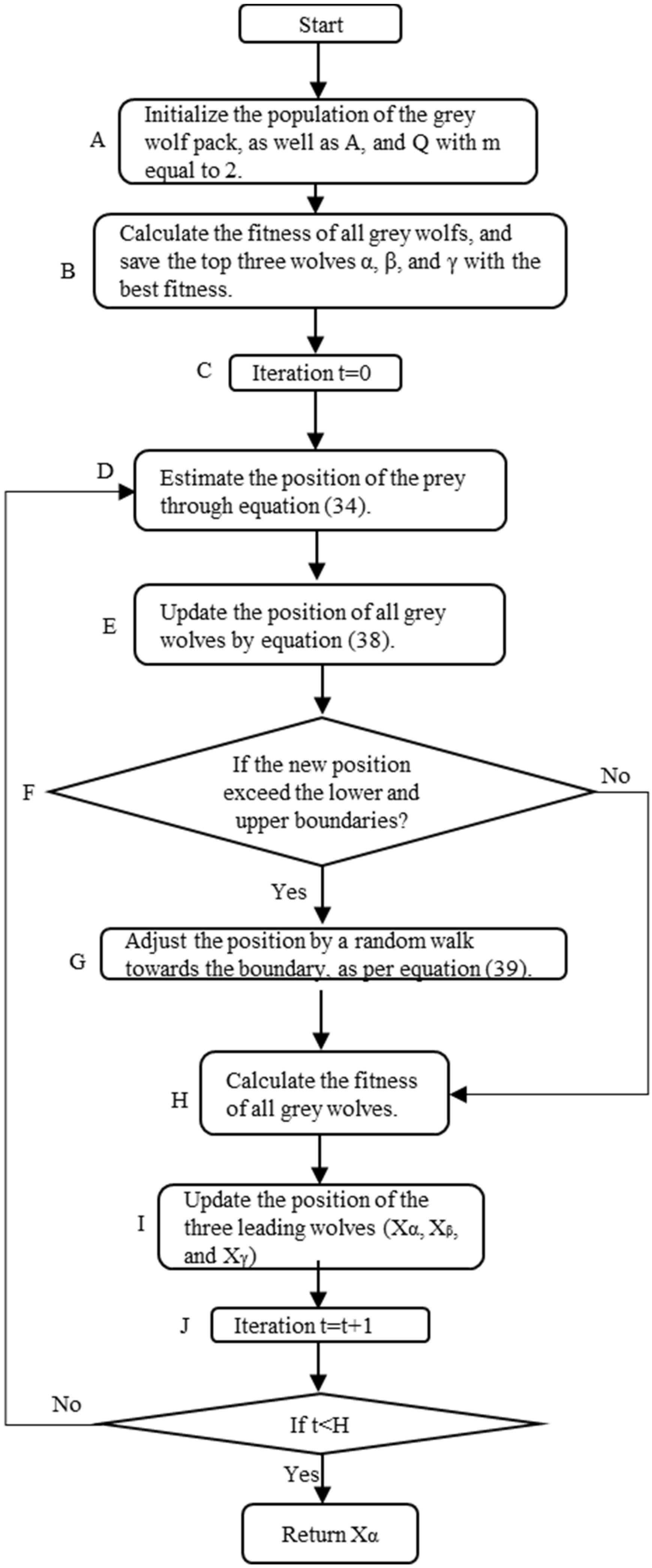


| Type | Parameters/Variables | Description/Settings |
|---|---|---|
| Input parameters | Critical for the distribution system model | |
| Output parameters | , , , , and | Critical for the objective function |
| Decision variables | Determine the sizes of BESSs in MVA with a unity power factor. | |
| Determine the locations of BESSs in the grid. | ||
| EGWO parameters | Settings: [–2, 2], [0, 1] | |
| Settings: | ||
| EGWO bounds | Settings: lb1 = 0.1 MVA and ub1 = 2 MVA Settings: lb2 = 0 and ub2 = 1 |
| Case Studies | Apparent Power per BESS (MVA) and Their Sites | VDI (%) | LLI (%) | (MVA) | (USD/Year) | Total BESS Size (MWh) | Objective Function Value (USD/Year) |
|---|---|---|---|---|---|---|---|
| Case 1: | No BESS | 100.813 | 256.192 | 0.214 | 407,860 | – | 959,529.845 |
| Case 2a: | BESS03, BESS06, BESS07, BESS08, BESS10, BESS11, BESS24, BESS27, BESS28, BESS30, BESS31, BESS32, BESS33, MVA for each BESS = 0.118 | 59.637 | 218.294 | 0.156 | 327,352 | 1.53 | 777,590.108 |
| Case 2b: | BESS03, BESS06, BESS07, BESS11, BESS12, BESS13, BESS14, BESS17, BESS19, BESS22, BESS23, BESS24, BESS32, BESS33, MVA for each BESS = 0.184 | 40.834 | 231.279 | 0.174 | 301,029 | 2.571 | 832,955.828 |
| Case 3a: | BESS03 = 0.154, BESS06 = 0.140, BESS07 = 0.212, BESS10 = 0.101, BESS12 = 0.221, BESS15 = 0.123, BESS16 = 0.141, BESS20 = 0.102, BESS21 = 0.228, BESS32 = 0.117, BESS33 = 0.123 | 63.918 | 217.094 | 0.16 | 343,117 | 1.662 | 807,263.689 |
| Case 3b: | BESS03 = 0.113, BESS06 = 0.148, BESS07 = 0.221, BESS10 = 0.153, BESS11 = 0.144, BESS18 = 0.445, BESS21 = 0.1, BESS25 = 0.251, BESS26 = 0.262, BESS27 = 0.105, BESS28 = 0.149, BESS30 = 0.202, BESS32 = 0.111, BESS33 = 0.132 | 40.646 | 232.682 | 0.177 | 309,181 | 2.535 | 845,109.939 |
| Case 4: | No BESS | 100.993 | 309.421 | 0.220 | 445,480 | – | 1,014,773.731 |
| Case 5a: | BESS05, BESS06, BESS07, BESS08, BESS09, BESS18, BESS24, BESS25, BESS26, BESS29, BESS30, BESS31, BESS32, BESS33, MVA for each BESS = 0.112 | 69.589 | 265.765 | 0.163 | 331,112 | 1.573 | 801,296.52 |
| Case 5b: | BESS03, BESS04, BESS06, BESS07, BESS08, BESS09, BESS14, BESS16, BESS18, BESS19, BESS20, BESS21, BESS30, BESS31, BESS32, BESS33, MVA for each BESS = 0.172 | 23.312 | 291.633 | 0.194 | 308,901 | 2.749 | 8,941,82.058 |
| Case 6a: | BESS02 = 0.127, BESS03 = 0.161, BESS06 = 0.232, BESS08 = 0.131, BESS10 = 0.159, BESS11 = 0.140, BESS17 = 0.158, BESS28 = 0.232, BESS29 = 0.108, BESS32 = 0.115, BESS33 = 0.157 | 67.519 | 266.914 | 0.176 | 355,030 | 1.72 | 863,067.735 |
| Case 6b: | BESS02 = 0.151, BESS05 = 0.183, BESS06 = 0.332, BESS08 = 0.241, BESS10 = 0.237, BESS11 = 0.221, BESS21 = 0.119, BESS22 = 0.1, BESS25 = 0.138, BESS26 = 0.126, BESS27 = 0.117, BESS29 = 0.142, BESS30 = 0.159, BESS31 = 0.218, BESS32 = 0.162, BESS33 = 0.233 | 27.321 | 291.213 | 0.209 | 319,687 | 2.881 | 945,827.482 |
| Cases Comparison | VDI Ratio | LLI Ratio | Ratio | Ratio | Total BESS Size Ratio | Objective Function Value Ratio |
|---|---|---|---|---|---|---|
| Case 3a:2a | 1.072 | 0.995 | 1.026 | 1.048 | 1.086 | 1.038 |
| Case 3b:2b | 0.995 | 1.006 | 1.017 | 1.027 | 0.986 | 1.015 |
| Case 6a:5a | 0.970 | 1.004 | 1.080 | 1.072 | 1.093 | 1.077 |
| Case 6b:5b | 1.172 | 0.999 | 1.077 | 1.035 | 1.048 | 1.058 |
| Optimization Statistics | Apparent Power per BESS (MVA) and Their Sites | VDI (%) | LLI (%) | (MVA) | (USD/Year) | Total BESS Size (MWh) | Objective Function Value (USD/Year) |
|---|---|---|---|---|---|---|---|
| Investigation category I: uniform size BESS allocation | |||||||
| EGWO best | BESS03, BESS06, BESS07, BESS08, BESS10, BESS11, BESS24, BESS27, BESS28, BESS30, BESS31, BESS32, BESS33, MVA for each BESS = 0.118 | 59.637 | 218.294 | 0.156 | 327,352 | 1.530 | 776,708.934 |
| EGWO worst | BESS03, BESS06, BESS07, BESS08, BESS10, BESS11, BESS24, BESS27, BESS28, BESS30, BESS31, BESS32, BESS33, MVA for each BESS = 0.120 | 60.288 | 221.805 | 0.160 | 326,672 | 1.562 | 787,222.024 |
| EGWO mean | BESS03, BESS06, BESS07, BESS08, BESS10, BESS11, BESS24, BESS27, BESS28, BESS30, BESS31, BESS32, BESS33, MVA for each BESS = 0.118 | 59.716 | 219.686 | 0.158 | 327,158 | 1.539 | 781,880.637 |
| 2254.229 | |||||||
| GWO best | BESS03, BESS06, BESS07, BESS08, BESS10, BESS11, BESS24, BESS27, BESS28, BESS30, BESS31, BESS32, BESS33, MVA for each BESS = 0.118 | 59.717 | 219.135 | 0.156 | 328,066 | 1.534 | 777,584.154 |
| GWO worst | BESS03, BESS06, BESS07, BESS08, BESS10, BESS11, BESS24, BESS27, BESS28, BESS30, BESS31, BESS32, BESS33, MVA for each BESS = 0.120 | 60.531 | 222.375 | 0.161 | 327,283 | 1.563 | 790,407.7772 |
| GWO mean | BESS03, BESS06, BESS07, BESS08, BESS10, BESS11, BESS24, BESS27, BESS28, BESS30, BESS31, BESS32, BESS33, MVA for each BESS = 0.119 | 60.279 | 220.224 | 0.159 | 327,626 | 1.547 | 785,136.4344 |
| 3168.572 | |||||||
| PSO best | BESS03, BESS06, BESS07, BESS08, BESS10, BESS11, BESS24, BESS27, BESS28, BESS30, BESS31, BESS32, BESS33, MVA for each BESS = 0.119 | 59.827 | 220.335 | 0.157 | 329,390 | 1.541 | 781,691.030 |
| PSO worst | BESS03, BESS06, BESS07, BESS08, BESS10, BESS11, BESS24, BESS27, BESS28, BESS30, BESS31, BESS32, BESS33, MVA for each BESS = 0.120 | 60.748 | 222.586 | 0.163 | 329,537 | 1.565 | 797,763.171 |
| PSO mean | BESS03, BESS06, BESS07, BESS08, BESS10, BESS11, BESS24, BESS27, BESS28, BESS30, BESS31, BESS32, BESS33, MVA for each BESS = 0.120 | 61.427 | 220.659 | 0.160 | 329,366 | 1.557 | 789,727.676 |
| 3801.475 | |||||||
| Investigation category I: non-uniform size BESS allocation | |||||||
| EGWO best | BESS03 = 0.154, BESS06 = 0.140, BESS07 = 0.212, BESS10 = 0.101, BESS12 = 0.221, BESS15 = 0.123, BESS16 = 0.141, BESS20 = 0.102, BESS21 = 0.228, BESS32 = 0.117, BESS33 = 0.123 | 63.918 | 217.094 | 0.160 | 343,117 | 1.662 | 806,494.357 |
| EGWO worst | BESS03 = 0.170, BESS06 = 0.144, BESS07 = 0.201, BESS10 = 0.111, BESS12 = 0.227, BESS15 = 0.132, BESS16 = 0.144, BESS20 = 0.117, BESS21 = 0.202, BESS32 = 0.122, BESS33 = 0.124 | 64.534 | 218.904 | 0.164 | 342,514 | 1.694 | 817,002.887 |
| EGWO mean | BESS03 = 0.165, BESS06 = 0.147, BESS07 = 0.207, BESS10 = 0.106, BESS12 = 0.217, BESS15 = 0.133, BESS16 = 0.143, BESS20 = 0.109, BESS21 = 0.214, BESS32 = 0.108, BESS33 = 0.113 | 64.441 | 217.825 | 0.164 | 343,248 | 1.664 | 816,784.140 |
| 2803.794 | |||||||
| GWO best | BESS03 = 0.179, BESS06 = 0.14, BESS07 = 0.173, BESS10 = 0.105, BESS12 = 0.222, BESS15 = 0.126, BESS16 = 0.131, BESS20 = 0.109, BESS21 = 0.222, BESS32 = 0.134, BESS33 = 0.122 | 64.204 | 217.155 | 0.16 | 343,325 | 1.664 | 806,769.3473 |
| GWO worst | BESS03 = 0.164, BESS06 = 0.143, BESS07 = 0.209, BESS10 = 0.127, BESS12 = 0.243, BESS15 = 0.112, BESS16 = 0.142, BESS20 = 0.108, BESS21 = 0.224, BESS32 = 0.129, BESS33 = 0.128 | 65.062 | 219.344 | 0.165 | 342,104 | 1.727 | 820,125.514 |
| GWO mean | BESS03 = 0.173, BESS06 = 0.135, BESS07 = 0.221, BESS10 = 0.12, BESS12 = 0.22, BESS15 = 0.134, BESS16 = 0.136, BESS20 = 0.103, BESS21 = 0.228, BESS32 = 0.114, BESS33 = 0.106 | 65.166 | 218.193 | 0.164 | 342,756 | 1.69 | 817,100.0288 |
| 3472.036 | |||||||
| PSO best | BESS03 = 0.160, BESS06 = 0.138, BESS07 = 0.223, BESS10 = 0.109, BESS12 = 0.225, BESS15 = 0.127, BESS16 = 0.136, BESS20 = 0.1, BESS21 = 0.213, BESS32 = 0.1, BESS33 = 0.134 | 64.666 | 217.269 | 0.160 | 343,460 | 1.665 | 806,946.377 |
| PSO worst | BESS03 = 0.166, BESS06 = 0.144, BESS07 = 0.219, BESS10 = 0.149, BESS12 = 0.256, BESS15 = 0.112, BESS16 = 0.151, BESS20 = 0.102, BESS21 = 0.237, BESS32 = 0.108, BESS33 = 0.122 | 66.225 | 219.982 | 0.168 | 341,361 | 1.769 | 828,231.884 |
| PSO mean | BESS03 = 0.158, BESS06 = 0.138, BESS07 = 0.223, BESS10 = 0.130, BESS12 = 0.225, BESS15 = 0.127, BESS16 = 0.156, BESS20 = 0.1, BESS21 = 0.233, BESS32 = 0.1, BESS33 = 0.127 | 66.179 | 218.974 | 0.165 | 342,384 | 1.719 | 820,163.831 |
| 4903.673 | |||||||
| Investigation category II: uniform size BESS allocation | |||||||
| EGWO best | BESS05, BESS06, BESS07, BESS08, BESS09, BESS18, BESS24, BESS25, BESS26, BESS29, BESS30, BESS31, BESS32, BESS33, MVA for each BESS = 0.112 | 69.589 | 265.765 | 0.163 | 331,112 | 1.573 | 801,762.079 |
| EGWO worst | BESS05, BESS06, BESS07, BESS08, BESS09, BESS18, BESS24, BESS25, BESS26, BESS29, BESS30, BESS31, BESS32, BESS33, MVA for each BESS = 0.115 | 70.355 | 270.044 | 0.170 | 330,417 | 1.607 | 819,900.770 |
| EGWO mean | BESS05, BESS06, BESS07, BESS08, BESS09, BESS18, BESS24, BESS25, BESS26, BESS29, BESS30, BESS31, BESS32, BESS33, MVA for each BESS = 0.114 | 69.680 | 267.466 | 0.168 | 330,649 | 1.594 | 814,582.039 |
| 3681.945 | |||||||
| GWO best | BESS05, BESS06, BESS07, BESS08, BESS09, BESS18, BESS24, BESS25, BESS26, BESS29, BESS30, BESS31, BESS32, BESS33, MVA for each BESS = 0.113 | 69.803 | 266.211 | 0.164 | 333,676 | 1.581 | 807,104.5086 |
| GWO worst | BESS05, BESS06, BESS07, BESS08, BESS09, BESS18, BESS24, BESS25, BESS26, BESS29, BESS30, BESS31, BESS32, BESS33, MVA for each BESS = 0.117 | 70.61 | 269.904 | 0.171 | 332,230 | 1.631 | 824,944.8592 |
| GWO mean | BESS05, BESS06, BESS07, BESS08, BESS09, BESS18, BESS24, BESS25, BESS26, BESS29, BESS30, BESS31, BESS32, BESS33, MVA for each BESS = 0.114 | 70.193 | 267.448 | 0.169 | 332,870 | 1.602 | 819,563.6258 |
| 4782.519 | |||||||
| PSO best | BESS05, BESS06, BESS07, BESS08, BESS09, BESS18, BESS24, BESS25, BESS26, BESS29, BESS30, BESS31, BESS32, BESS33, MVA for each BESS = 0.113 | 69.965 | 267.053 | 0.165 | 336,410 | 1.588 | 812,605.067 |
| PSO worst | BESS05, BESS06, BESS07, BESS08, BESS09, BESS18, BESS24, BESS25, BESS26, BESS29, BESS30, BESS31, BESS32, BESS33, MVA for each BESS = 0.119 | 71.035 | 269.777 | 0.173 | 336,545 | 1.660 | 835,158.116 |
| PSO mean | BESS05, BESS06, BESS07, BESS08, BESS09, BESS18, BESS24, BESS25, BESS26, BESS29, BESS30, BESS31, BESS32, BESS33, MVA for each BESS = 0.115 | 70.917 | 267.427 | 0.171 | 336,383 | 1.611 | 828,384.203 |
| 5216.346 | |||||||
| Investigation category II: non-uniform size BESS allocation | |||||||
| EGWO best | BESS02 = 0.127, BESS03 = 0.161, BESS06 = 0.232, BESS08 = 0.131, BESS10 = 0.159, BESS11 = 0.140, BESS17 = 0.158, BESS28 = 0.232, BESS29 = 0.108, BESS32 = 0.115, BESS33 = 0.157 | 67.519 | 266.914 | 0.176 | 355,030 | 1.720 | 862,798.837 |
| EGWO worst | BESS02 = 0.151, BESS03 = 0.154, BESS06 = 0.212, BESS08 = 0.132, BESS10 = 0.157, BESS11 = 0.152, BESS17 = 0.155, BESS28 = 0.248, BESS29 = 0.109, BESS32 = 0.111, BESS33 = 0.162 | 68.167 | 269.130 | 0.183 | 354,391 | 1.743 | 880,563.532 |
| EGWO mean | BESS02 = 0.142, BESS03 = 0.159, BESS06 = 0.231, BESS08 = 0.133, BESS10 = 0.159, BESS11 = 0.156, BESS17 = 0.155, BESS28 = 0.230, BESS29 = 0.1, BESS32 = 0.1, BESS33 = 0.158 | 68.072 | 267.795 | 0.182 | 355,172 | 1.721 | 878,105.437 |
| 4087.372 | |||||||
| GWO best | BESS02 = 0.184, BESS03 = 0.189, BESS06 = 0.211, BESS08 = 0.144, BESS10 = 0.161, BESS11 = 0.126, BESS17 = 0.159, BESS28 = 0.245, BESS29 = 0.115, BESS32 = 0.115, BESS33 = 0.1 | 67.932 | 266.971 | 0.175 | 356,921 | 1.749 | 863,054.3303 |
| GWO worst | BESS02 = 0.15, BESS03 = 0.149, BESS06 = 0.198, BESS08 = 0.151, BESS10 = 0.145, BESS11 = 0.145, BESS17 = 0.168, BESS28 = 0.26, BESS29 = 0.108, BESS32 = 0.107, BESS33 = 0.201 | 68.859 | 269.61 | 0.185 | 355,641 | 1.784 | 888,104.5267 |
| GWO mean | BESS02 = 0.135, BESS03 = 0.164, BESS06 = 0.223, BESS08 = 0.15, BESS10 = 0.149, BESS11 = 0.146, BESS17 = 0.149, BESS28 = 0.24, BESS29 = 0.099, BESS32 = 0.109, BESS33 = 0.184 | 68.212 | 268.275 | 0.183 | 355,560 | 1.752 | 881,962.4297 |
| 5653.736 | |||||||
| PSO best | BESS02 = 0.153, BESS03 = 0.179, BESS06 = 0.231, BESS08 = 0.153, BESS10 = 0.168, BESS11 = 0.131, BESS17 = 0.164, BESS28 = 0.242, BESS29 = 0.1, BESS32 = 0.1, BESS33 = 0.102 | 68.153 | 267.013 | 0.175 | 357,870 | 1.723 | 863,228.487 |
| PSO worst | BESS02 = 0.162, BESS03 = 0.165, BESS06 = 0.202, BESS08 = 0.164, BESS10 = 0.151, BESS11 = 0.148, BESS17 = 0.177, BESS28 = 0.259, BESS29 = 0.114, BESS32 = 0.101, BESS33 = 0.192 | 69.795 | 270.351 | 0.187 | 357,798 | 1.837 | 896,928.444 |
| PSO mean | BESS02 = 0.156, BESS03 = 0.182, BESS06 = 0.230, BESS08 = 0.157, BESS10 = 0.151, BESS11 = 0.144, BESS17 = 0.160, BESS28 = 0.238, BESS29 = 0.107, BESS32 = 0.1, BESS33 = 0.203 | 70.143 | 269.096 | 0.182 | 356,188 | 1.829 | 882,453.006 |
| 7252.429 | |||||||
| Investigation Category | BESS Allocation | EGWO Convergence | EGWO Computation Time (s) | GWO Convergence | GWO Computation Time (s) | PSO Convergence | PSO Computation Time (s) |
|---|---|---|---|---|---|---|---|
| I | Uniform BESS | After 239 iterations | 581 | 262 | 642 | After 293 iterations | 716 |
| Non-uniform BESS | After 340 iterations | 774 | 357 | 799 | After 428 iterations | 945 | |
| II | Uniform BESS | After 256 iterations | 611 | 285 | 681 | After 311 iterations | 742 |
| Non-uniform BESS | After 346 iterations | 810 | 367 | 821 | After 440 iterations | 983 |
| Improved Cost Saving of EIC (%) | Improved Cost Saving of Cost of EENS (%) | Improved Cost Saving of TOC (%) | Reduced SAIDI (%) | |
|---|---|---|---|---|
| Case 1 | – | – | – | – |
| Case 2a | 20.010 | 19.536 | 19.739 | 14.522 |
| Case 2b | 26.314 | 25.997 | 26.193 | 23.781 |
| Case 3a | 15.694 | 15.923 | 15.874 | 11.806 |
| Case 3b | 23.981 | 24.240 | 24.194 | 29.138 |
| Case 4 | – | – | – | – |
| Case 5a | 25.742 | 25.577 | 25.673 | 24.770 |
| Case 5b | 30.577 | 30.547 | 30.659 | 30.245 |
| Case 6a | 19.838 | 20.480 | 20.304 | 20.634 |
| Case 6b | 28.252 | 27.933 | 28.238 | 34.185 |
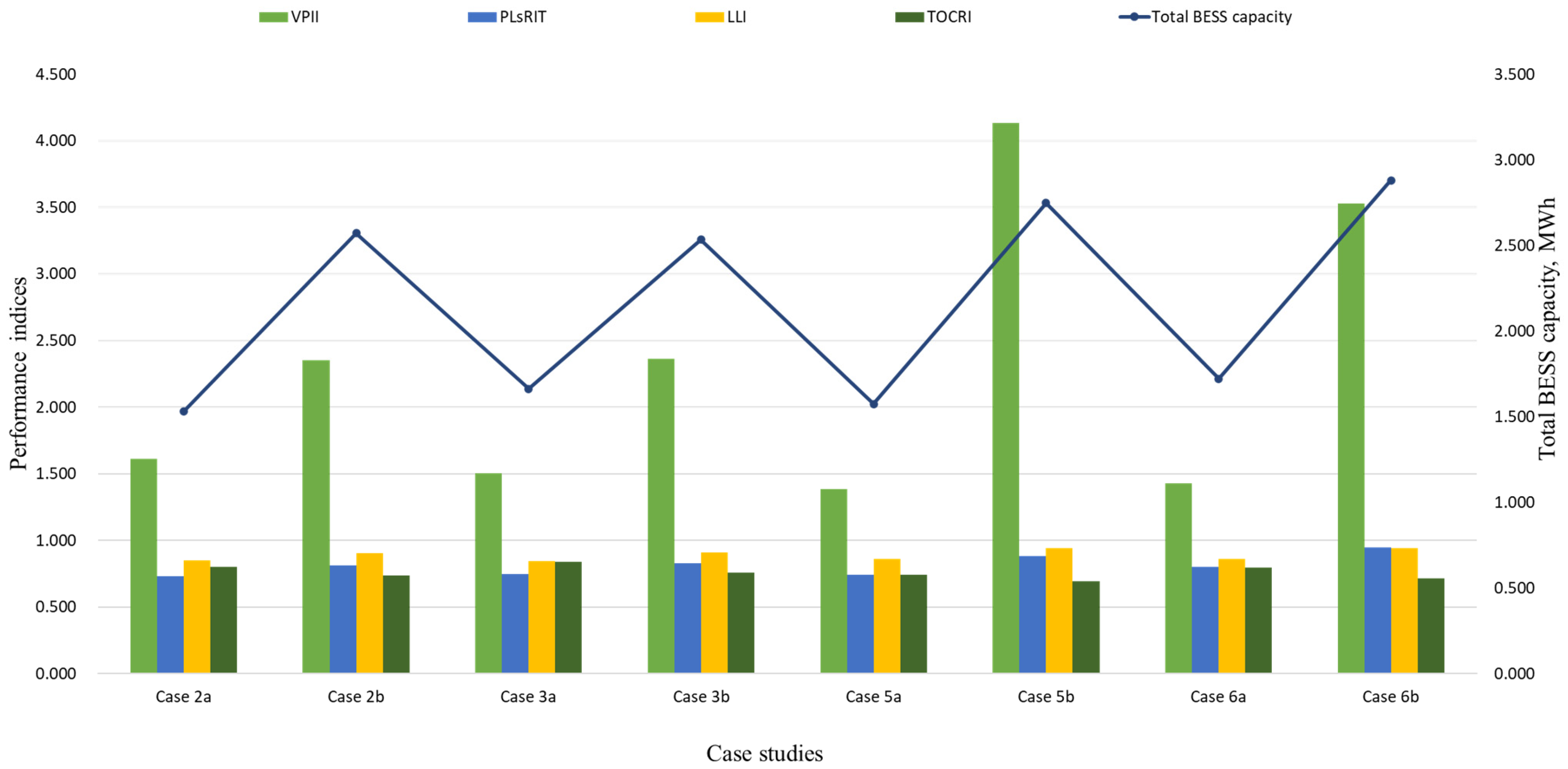
| Case Studies | VPII | LLI | TOCRI | |||
|---|---|---|---|---|---|---|
| Case 1 | – | – | – | – | – | – |
| Case 2a | 1.609 | 0.716 | 0.748 | 0.729 | 0.852 | 0.803 |
| Case 2b | 2.350 | 0.796 | 0.838 | 0.813 | 0.903 | 0.738 |
| Case 3a | 1.501 | 0.729 | 0.775 | 0.748 | 0.847 | 0.841 |
| Case 3b | 2.361 | 0.806 | 0.855 | 0.827 | 0.908 | 0.758 |
| Case Studies | VPII | LLI | TOCRI | |||
|---|---|---|---|---|---|---|
| Case 4 | – | – | – | – | – | – |
| Case 5a | 1.385 | 0.740 | 0.742 | 0.741 | 0.859 | 0.743 |
| Case 5b | 4.135 | 0.875 | 0.917 | 0.882 | 0.943 | 0.693 |
| Case 6a | 1.428 | 0.790 | 0.842 | 0.800 | 0.863 | 0.797 |
| Case 6b | 3.528 | 0.938 | 0.997 | 0.950 | 0.941 | 0.718 |
Disclaimer/Publisher’s Note: The statements, opinions and data contained in all publications are solely those of the individual author(s) and contributor(s) and not of MDPI and/or the editor(s). MDPI and/or the editor(s) disclaim responsibility for any injury to people or property resulting from any ideas, methods, instructions or products referred to in the content. |
© 2023 by the authors. Licensee MDPI, Basel, Switzerland. This article is an open access article distributed under the terms and conditions of the Creative Commons Attribution (CC BY) license (https://creativecommons.org/licenses/by/4.0/).
Share and Cite
Zhang, D.; Shafiullah, G.; Das, C.K.; Wong, K.W. Optimal Allocation of Battery Energy Storage Systems to Enhance System Performance and Reliability in Unbalanced Distribution Networks. Energies 2023, 16, 7127. https://doi.org/10.3390/en16207127
Zhang D, Shafiullah G, Das CK, Wong KW. Optimal Allocation of Battery Energy Storage Systems to Enhance System Performance and Reliability in Unbalanced Distribution Networks. Energies. 2023; 16(20):7127. https://doi.org/10.3390/en16207127
Chicago/Turabian StyleZhang, Dong, GM Shafiullah, Choton Kanti Das, and Kok Wai Wong. 2023. "Optimal Allocation of Battery Energy Storage Systems to Enhance System Performance and Reliability in Unbalanced Distribution Networks" Energies 16, no. 20: 7127. https://doi.org/10.3390/en16207127
APA StyleZhang, D., Shafiullah, G., Das, C. K., & Wong, K. W. (2023). Optimal Allocation of Battery Energy Storage Systems to Enhance System Performance and Reliability in Unbalanced Distribution Networks. Energies, 16(20), 7127. https://doi.org/10.3390/en16207127