Abstract
This article focuses on increasing the computational efficiency of 3D multi-static magnetic finite element analysis (FEA) for electrical machines (EMs), which have a magnetic field evolving in 3D space. Although 3D FEA is crucial for analyzing these machines and their operational behavior, it is computationally expensive. A novel approach is proposed in order to solve the magnetic field equations by exclusively using the magnetic scalar potential. For this purpose, virtual variable permanent magnets (vPMs) are introduced to model the impact of the machine’s coils. The effect on which this approach is based is derived from and explained by Maxwell’s equations. To validate the new approach, an axial flux machine (AFM) is simulated using both 2D and 3D FEA with the magnetic vector potential and current-carrying coils as a reference. The results demonstrate a high level of agreement between the new approach and the reference simulations as well as an acceleration of the computation by a factor of 15 or even more. Additionally, the research provides valuable insights into meshing techniques and torque calculation for EMs in FEA.
1. Introduction
In rotary electrical machines (EMs), torque is generated by the interaction of the magnetic rotor field and the stator field. Depending on the alignment and orientation of these fields, EMs are distinguished into different topologies. The most common topology is the radial flux machine (RFM), where the magnetic field propagates mainly in the plane orthogonal to the axis of rotation. For the electromagnetic modeling and simulation of such machines, therefore, only a 2D cross-section of the machine is simulated [1,2]. The field components in the axial direction, which occur mainly at the end windings, are neglected or replaced by additional computationally efficient models [3]. In addition to the RFM, other topologies exist as well, namely the axial flux machine (AFM) and the transverse flux machine (TFM). Both topologies offer potential advantages, especially regarding torque density and low-speed applications [4,5,6]. Because of the different orientations of the magnetic field and the increased geometrical complexity for both topologies, all spatial components of the magnetic field are to be considered to accurately describe the machine’s behavior [7]. Hence, instead of a 2D problem, a 3D problem has to be solved. Apart from analytical modeling techniques, 3D finite element analysis (FEA) is a popular and simple-to-set-up modeling technique to investigate these machine topologies. However, due to the additional dimension, the computational effort increases cubically instead of quadratically when the solving mesh is refined. Especially for the optimization of the machine design during the development, a significant number of simulations with a significant variation in geometric shape is required. Although 3D FEA is well-suited to model arbitrary shapes, the computational effort is a limiting factor for its application. Based on common FEM-based approaches to solving Maxwell’s equations in 3D space, a new approach to significantly reduce the simulation time of 3D FEA is presented and exemplarily investigated using an AFM.
1.1. Maxwell’s Equations
In EMs, the electromagnetic fields vary in time. Due to the relatively low frequency of variation, the wavelengths of potential electromagnetic waves are significantly larger than the dimensions of the EM. For these reasons, the quasi-static Maxwell’s equations neglecting the displacement current are used to model the electric and magnetic fields [8,9].
In these equations, H describes the magnetic field, B is the magnetic flux density, E is the electric field strength, J is the current density, and ∇ is the nabla operator.
Furthermore, the propagation of the fields in different materials is determined by the material laws
Due to saturation, the permeability of the material depends on the H-field and is assumed to be nonlinear in the soft magnetic components. The electrical conductivity is assumed to be linear. Instead of using a nonlinear function for , a nonlinear B-H curve directly describes the relation between B and H [8,10,11,12].
For magnetically isotropic materials, the nonlinear effect only depends on the magnitude of the H-field .
Although f is a vector function, f* is a scalar function multiplied with a unit vector pointing in the direction of the H-field. When considering nonlinear effects, a derivation of the iterative Newton method is to be used to solve the nonlinear equations, further increasing the simulation time [13]. For linear and nonlinear systems, the basic process to solve the coupled differential equations is described subsequently.
1.2. Eddy Currents and Multi-Static Simulations
By solving the full set of Maxwell’s Equations (1)–(4) a detailed analysis of the machine’s transient response including the complete effects of eddy currents is possible. The major drawback is its computational complexity. An alternative is to decouple Maxwell’s equations, first solving the magnetostatic problem and then solving the eddy currents on the basis of the electric Equations (1), (4), and (6). This approach is investigated in [14] and [15]. In [14], the finite difference method is used to solve the three electric equations, leading to an 11 times faster simulation and an error <12% for the eddy current losses compared to the transient simulation. In [15], an analytical solution for the eddy current equations is proposed, being able to calculate the eddy current losses for simple geometries based on closed analytical equations. A third approach exists, which not directly solves the eddy current equations from above, but instead creates a network of resistances and voltage sources in an electric equivalent circuit [16,17]. Extensive knowledge exists to solve electric circuits efficiently and depending on the resolution of the network, the solution is more comprehensible than the FEA.
Despite the mentioned open loop methods, the approaches in [15,17] also enable the feedback of the calculated eddy currents on the magnetic field, i.e., the magnetic reaction field is considered. The influences of the reaction field vary with the operating point and are mainly dependent on the excitation of the machine [17].
In summary, there are multiple methods able to consider the losses and transient effects of eddy currents based on an initial magnetostatic simulation with tunable accuracy. Compared to the fully coupled simulation of Maxwell’s equations, this leads to a significant reduction in simulation time. Because of an accelerated simulation and since eddy currents can be calculated in post-processing with the methods given in this subchapter, eddy currents are not considered in this article. Therefore, the focus of this article is exclusively on the magnetostatic field problem which is solved with multi-static 3D FEA.
1.3. Magnetic Vector Potential
The magnetostatic field problem is described in (2), (3), and (7) [1,8,18,19]. To solve this system of equations efficiently with a reduced number of equations, the magnetic vector potential A is introduced [19] and defined by the equation
The magnetic vector potential fulfills Equation (3) of Maxwell’s equations by definition. Furthermore, the constant current density in (2) is generated by an external source and is assumed to fulfill (4). Therefore, Ampère’s law (2) and the material law (7) are the only remaining equations to be solved. Nevertheless, the magnetic vector potential consists of three components for a 3D problem, still leading to a high number of dependent variables to be solved, especially for a fine mesh and a large simulation space.
1.4. Magnetic Scalar Potential
If there are no free currents (J = 0) and no time dependency of the magnetic field, Equation (2) becomes
and a simplified approach to solving the magnetic field exists based on the magnetic scalar potential [18,19]. As (10) suggests, the rotation of the H-field is zero and therefore it can be described by the gradient of the magnetic scalar potential .
As the name suggests, the scalar potential is one-dimensional and leads to a significantly decreased computational effort compared to the three-dimensional vector potential. For magnetostatic problems without currents but including permanent magnets, the magnetic scalar potential represents the most efficient approach to calculating the resulting magnetic fields.
1.5. Mixed Formulations and Discontinuities in the Magnetic Scalar Potential
The mixed formulation method is another approach to reduce the computational complexity of solving magnetic field problems in 3D space. With this method, the model is divided into multiple domains and different solution strategies, i.e., different solution variables are chosen for each domain. Especially, if one solution strategy is based on the magnetic scalar potential, a decrease in the simulation time is possible.
Firstly, in the context of superconductors, the magnetic field H is directly used as a solution variable in all regions containing conductive materials [20]. This is referenced as H-formulation. In non-conductive regions, such as air, the magnetic scalar potential is used. Notably, when regions with the H-formulation are enclosed by regions utilizing the scalar potential, special attention has to be paid to ensure that Ampère’s law continues to be fulfilled. In [21,22], thin cuts are used to introduce a discontinuous magnetic scalar potential thereby considering the magnetomotive force (MMF) of the conductors. In detail, the surface spanned by the conductors of the coil is used as a cut surface. Between the two sides of the cut surface, a difference in the magnetic potential, which corresponds to the MMF of the conductor, is applied. This approach has demonstrated computational speed-ups of up to seven times compared to the full H-formulation while achieving comparable accuracy [21].
A basic 2D example is illustrated in Figure 1 where a current flows in the opposite direction through the cross sections of two conductors, which are modeled with the H-formulation. For the surrounding air domain, the magnetic scalar potential is used and one thin cut is introduced between both conductors to induce the MMF of the conductors.
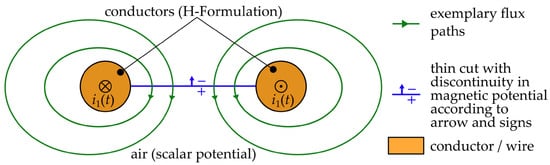
Figure 1.
Mixed formulation with thin cuts in the air region to satisfy Ampère’s law orientated on [21].
Without the thin cut, Ampère’s law formulated for the drawn flux paths is incorrect because the enclosed current within the path loops is not considered. Inaccurate simulation results would be the consequence. The discontinuity of the scalar potential over the thin cut replicates the enclosed current of the drawn flux path loops and thereby solves this problem.
Another use case of mixed formulations is the simulation of rotating EMs as advocated by COMSOL [23]. In areas involving windings, Ampère’s law is employed to map the effect of current density on the H-field. The magnetic vector potential is used for the solution in these regions. Conversely, in regions where windings are not present, such as air and the permanent magnet-excited rotor, the magnetic scalar potential is used. Notably, it is crucial to avoid enclosing regions using the vector potential with regions using the scalar potential otherwise the introduction of discontinuities in the region of the scalar potential would be necessary as well. Moreover, in the air gap, the sliding interpolation interface and the boundaries with periodic conditions benefit from the use of the magnetic scalar potential due to the increased robustness of the solving process.
2. Concept
In this work, the magnetic scalar potential is used in the total simulation space instead of partial regions in order to further reduce the computational effort of 3D FEA. Therefore, the coils within the machine must be modeled by a different approach so that their effect remains in the model.
A first and straightforward approach to introduce the MMF of the coils is based on the mixed-formulation simulation of superconductors mentioned in Section 1.5. The new approach shall be applicable for EMs with a soft magnetic stator only. So, the magnetic field is concentrated in the soft magnetic components. Therefore, with good approximation, the MMF can be concentrated on the soft magnetic core as well. Furthermore, the regions with the H-Formulation used by [21,22] to model the conductors are assumed to be neglectable and the MMF of the conductors is solely represented by thin cuts through the soft magnetic core.
Figure 2a illustrates an example with a basic magnetic circuit consisting of a rectangular core and a coil with four windings. The thin cuts between the wires are represented by blue lines and the blue arrows indicate the direction of the MMF.
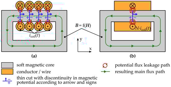
Figure 2.
Using thin cuts to substitute the effect of current-carrying coils for (a) a multi-wire coil and (b) a homogenized coil.
A problem occurs at the ends of the cuts, especially if the coils are not modeled as single wires but are instead modeled by a simplified body, as illustrated in Figure 2b. In this case, only one cut is needed but the effect of the MMF is concentrated, which can lead to a high leakage flux between both sides of the cut. This leakage flux does not occur in reality because the MMF is spread over the total length of the coil. To overcome this potential problem and enhance the model of coils for the magnetic scalar potential, the basic idea is developed further by using permanent magnets (PMs) instead of thin cuts. PMs are another source of MMF within a magnetic circuit, thereby potentially being able to reproduce the effect of a coil. Because real PMs are a static source of MMF and feature a low relative permeability, two changes must be introduced compared to real PMs so that a PM replicates a coil:
- 1.
- To simulate alternating current, the effect of the permanent magnet must also be variably adjustable. Therefore, the term “virtual variable permanent magnet” (vPM) is used for the new approach;
- 2.
- To replicate a soft magnetic core between the coil’s windings, the relative permeability of the vPM must be the same as the soft magnetic core. Hence, the relative permeability is significantly higher than that of a real magnet or is even nonlinear to model the saturation of the soft magnetic core.
Figure 3 illustrates how the new approach is integrated into the basic circuit from Figure 2. Although the coil is still shown, the current of the coil is not integrated into the simulation. Instead, the vPM is placed in the center of the coil over the full length of the coil and thereby replaces the soft magnetic core in this area as well as the MMF of the current.
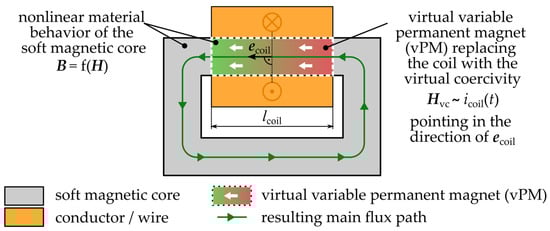
Figure 3.
Novel approach of using a vPM to substitute the effect of current-carrying coils for a homogenized coil.
Figure 4 shows a comparison of the B-H curves of a real PM and of the vPM in the one-dimensional case. Neglecting the temperature dependency, the hysteresis curve of a real PM illustrated in Figure 4a is static and the remanence as well as the coercivity, are constant. However, the vPM is described by the current-dependent virtual coercivity and the material law of the soft magnetic material f*. With a changing current, the virtual coercivity changes, and the B-H curve of the vPM in Figure 4b is moved horizontally, resulting in a changed MMF on the magnetic circuit.
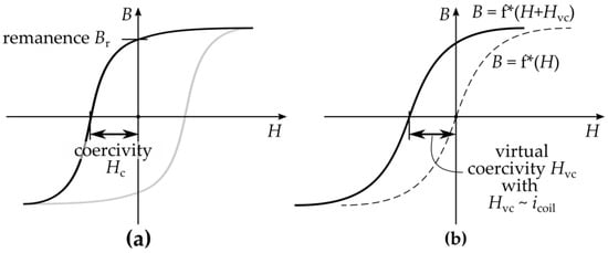
Figure 4.
Comparison of the BH curves of (a) a real PM and (b) a vPM.
In the 3D space, the virtual coercivity is defined as
Here, N is the number of windings, is the time-varying current through the coil the vPM replaces, and is the length of the coil in the direction of . The unit vector defines the direction of the vPM’s effect, which is derived by the direction of the current and the right-hand rule as described in Figure 5. Therefore, if the sign of the current changes, the direction of is inverted as well.
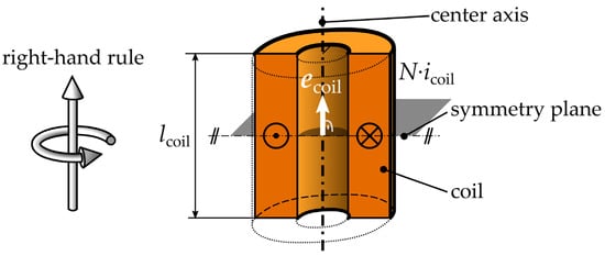
Figure 5.
Cross section of a simplified multi-turn coil indicating the current and the direction of the coil vector by the right-hand rule.
The virtual coercivity is introduced into the simulation space by creating an additional field which offsets the magnetic field .
In (13), the vector is the position vector of an arbitrary position in the simulation space and is the region of the vPM.
Figure 6 illustrates how the region of the vPM is derived for a simplified coil body. The coil region is defined by sweeping a rectangle R along a closed curve C which lies on a Euclidean plane P with the normal vector . The plane P is the same as the symmetry plane from Figure 5. The size of the rectangle R is defined by and where is the length of the rectangle in the direction of . The new approach is not limited to coils with this definition, so more sophisticated coil designs are to be investigated in future research. However, with this definition of the coils’ shape, concentrated coil designs of AFMs can be replicated. An exemplary coil body is shown in Figure 6a.
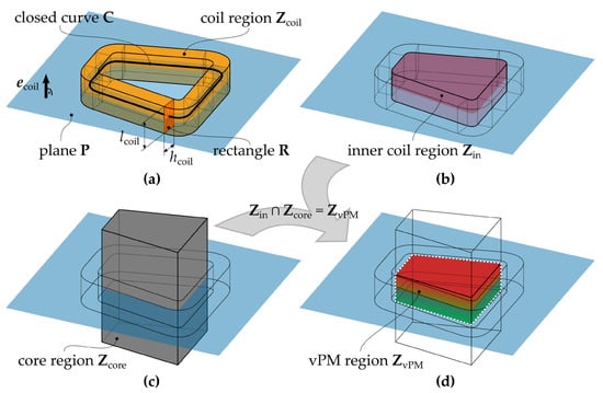
Figure 6.
Derivation of the vPM region for a simplified coil body, with (a) the definition of the simplified coil body, (b) the definition of the inner coil region, (c) an exemplary region of the soft magnetic core, and (d) the resulting region of the vPM.
The inner region of the coil shown in Figure 6b is derived by first extruding the section of the plane P which is bounded by the curve C. The extrusion is performed in both the positive and negative directions of over the length . then results as the set difference in the extruded region and . Finally, the region of the vPM is defined as the intersection of and the region of the soft magnetic core . Figure 6c gives an example for and Figure 6d illustrates the region of the vPM as a result of the intersection.
Considering the additional field the magnetic material law becomes
In the nonlinear case (14) becomes
using the nonlinear B-H curve from (7) and the adjusted magnetic field as input.
Although H itself fulfills (10) and thereby is solvable with (11) and the magnetic scalar potential, can be modified externally to ensure the adjusted Ampère’s law
For this reason, the effect of the current density of the coil is replicated in with the right definition of . Combining (10) and (16) the optimal definition of is derived in (17).
In summary, the solving process of the material law is decoupled from solving Ampère’s law. The latter has to be enforced externally by introducing vPMs into the simulation space. With the presented simplification of defining the vPMs only in the soft magnetic cores, the effect of the current density on the magnetic circuit is only modeled in this region neglecting the effect of the current density in the insulation and the winding cross section itself. Therefore, only for the paths passing through the full length of the vPM the adjusted Ampère’s law (16) is identically fulfilled as for the magnetic vector potential using current densities. However, because the magnetic flux is mainly focused on the soft magnetic materials this simplification is expected to be valid. In the following, this assumption is validated for an AFM using several FEM simulations in comparison to the magnetic vector potential and current densities as excitation.
3. Yokeless and Segmented Armature AFM
The new concept of vPMs and the associated assumptions have to be validated. For this purpose, an AFM in “Yokeless and Segmented Armature” (YASA) design is chosen as an example case. The basic structure of the magnetic components of a YASA AFM with one inner stator and two outer rotors is shown in Figure 7.
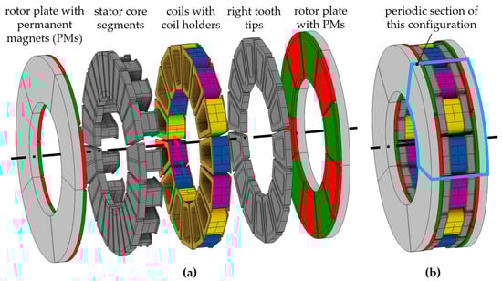
Figure 7.
A 3D view of the exemplary EM with (a) exploded view of the exemplary YASA AFM and (b) periodic section of this AFM configuration.
The magnetic rotor field is generated by permanent magnets that are mounted on the surface of the rotor discs creating five pole pairs as illustrated in Figure 7a. The rotor discs act as a yoke and close the magnetic circuit at the axial ends. The magnetic field of the stator is generated by a three-phase winding system. The single coils are wound around coil holders which are mounted on each of the 15 separated stator core segments. Additionally, the coil holders act as insulation between the windings and the soft magnetic cores. The resulting configuration of the AFM consisting of 15 stator segments and five pole pairs is based on the most basic configuration possible (3 segments and 1 pole pair) but extended to five periodic repetitions. One of these periodic sections is highlighted in Figure 7b.
The simple configuration is intended to reduce the complexity of the simulation and thus focus on the comparison of the solving approaches. A detailed view of a single periodic section of the YASA AFM is given in Figure 8. Furthermore, the figure consists of two sectional views where the main geometric parameters are defined.
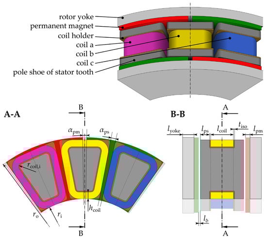
Figure 8.
Periodic section of the exemplary YASA AFM with two sectional views defining the main geometric parameters. The view A-A is perpendicular to the machine’s axis of rotation and the view B-B is aligned to the axis of rotation and the radial axis.
The values for the parameters of the nominal design of the AFM are given in Table 1. The nominal design is oriented on existing designs from [24,25] to validate the solving approach for a practically relevant design. Therefore, the soft magnetic material is also modeled by nonlinear magnetization curves, which are shown in Appendix A. Due to the 3D flux paths in the stator, soft magnetic composite (SMC) is often chosen as the material for the stator segments, because it features a moderate and isotropic magnetic permeability while reducing eddy current losses [26,27,28]. For the rotor, solid free-cutting steel 9S20K (material number 1.0711) is used instead, since the harmonics of the magnetic rotor field have low amplitudes compared to the stationary component, which already favors low eddy current losses.

Table 1.
Input parameters of the nominal design of the exemplary YASA AFM.
4. Simulation and Results
The new approach presented in Section 2 is investigated in the 2D and the 3D space. Due to the reduced computation time, the 2D space allows a detailed investigation of the mesh and a much higher mesh resolution. Therefore, the convergence of the solutions is tracked and numerical errors are neglected when comparing the modeling approaches. Furthermore, an investigation of the robustness of the modeling approaches against the change in geometrical parameters is possible. On the other hand, in 3D space, the mesh resolution is limited because the maximal available memory is already exceeded for moderate resolutions. For this reason, the numerical error is to be considered when comparing both modeling approaches.
All simulations presented in this chapter are performed using the “Rotating Machinery, Magnetic Interface” physics environment of the COMSOL Multiphysics® v6.1 software [29]. In this specific physics environment, the software enables the application of the magnetic scalar or vector potential, periodic boundary conditions to focus on a single periodic section, induced external current densities, homogenized multi-turn coils, and nonlinear soft magnetic materials. Furthermore, linear and nonlinear permanent magnets can be modeled by using a remanent flux density or a coercivity with a nonlinear shifted B-H curve, respectively. Both kinds of permanent magnets permit a variable remanent flux density or coercivity and therefore are well suited to implement the new approach with low effort.
Normally, EMs are simulated using an interpolation interface in the air gap, which is able to allow a relative movement between the rotor and the stator [1,18]. This interface is omitted for the validation because robustness issues of the nonlinear solver can occur if solved for the magnetic vector potential. Instead, the movement of the rotor is implemented by a step-by-step change in the geometry, which is why the geometry must be re-meshed in each step. Although this increases simulation time, the increased robustness and higher achievable accuracy are weighted more important for validation.
All simulations are based on sinusoidal 3-phase current resulting in an electrical load angle of 90 degrees. This represents the most basic operating point and ensures comparability between simulations.
4.1. 2D Simulations
The setup and geometry of the 2D simulation is illustrated in Figure 9. If the magnetic scalar potential is used, for each of the three coils a vPM with the same length as the coils ( replaces the soft magnetic core in the center. If the vector potential is used an external current density is applied to the coils and the soft magnetic core remains unmodified.
Figure 9.
vPMs replacing the three phase coils in the 2D simulation space and setup of an AFM.
As a simplifying assumption, the 2D geometry is generated in Cartesian coordinates and the geometric quantities are obtained from the rotary AFM for the equivalent radius, which is chosen to be the average radius of the magnetically active zone. This radius also is used to calculate the resulting torque from the output force of the Cartesian simulation. The height of the simulation space is set as the difference between the outer and inner radius of the active zone. Similar assumptions are found in the literature [5,30,31]. The error resulting from this assumption varies depending on the exact geometrical setup. Since the goal is not to obtain quantitatively comparable 2D and 3D simulations, but to obtain qualitatively comparable geometries and field distributions, this assumption is sufficient. Therefore, the validation is performed separately for the 2D and 3D space.
For 2D simulations, there is no significant speed-up of the magnetic scalar potential compared to the magnetic vector potential, because for the vector potential only the out-of-plane component is used to consider the out-of-plane current density. The other two components of the vector potential are neglected. Therefore, the only difference in the degrees of freedom (DOF) results from the different discretization of both potentials. Although the scalar potential is solved for node elements, the vector potential is solved for edge elements [32]. The different types of discretization lead to numerical errors between the solution strategies which are investigated in the following subsection.
4.1.1. Mesh Analysis and Torque Calculation Method
A useful indicator to observe the mesh convergence is the error between the solutions of the magnetic scalar potential and the magnetic vector potential when no electric load is applied. In this case, with no current densities, both solution strategies must lead to the same solution and the only possible error is a result of numerical errors. Since torque is one of the most important output quantities in the magnetic simulation of EMs, the error of the torque between both solution strategies is used to evaluate the mesh quality and convergence behavior.
As Figure 10 illustrates, the mesh refinement investigation consists of three dimensions: overall mesh detail, edge type, and the mesh refinement level of the edges (MRLE). Moreover, detailed views of the mesh are shown in the figure for two exemplary parameter combinations (I and II), highlighted in green and visualizing the differences between the parameter settings. The mesh view zone used for the detailed views of the mesh in Figure 10 is shown in Figure 9. As the name suggests, the “overall mesh detail” defines the mesh resolution in the total simulation space. If set to “extremely fine”, the mesh is finer on average compared to the “normal” setting. Near sharp edges, the other two parameters have a greater influence on the mesh, potentially reducing the risk of discontinuities. Mesh example I) in Figure 10 demonstrates that for the parameter “edge type” set to “edge fillet”, the sharp edges are rounded off with a small radius. Finally, the ascending parameter MRLE describes an increasing mesh resolution near sharp edges.
Figure 10.
Dimensions of the mesh refinement investigation with two mesh examples.
In addition to the mesh refinement dimensions, the torque calculation method is introduced as the fourth dimension of the investigation. The calculation of the torque is executed in post-processing after the magnetic field problem has been solved. Hence, the torque calculation is independent of the solution approach. Two calculation methods are distinguished:
- 1.
- The “Maxwell stress tensor (MST) method” is the classical method to compute the torque directly from the electromagnetic field. The MST torque is calculated with (18).
- 2.
- The “Arkkio torque method” is based on the original method proposed by Antero Arkkio [33]. The method is slightly modified and transformed to be used in the 2D space with Cartesian coordinates. The Arkkio torque is calculated with (19).
Both methods are based on the magnetic shear stress
from the MST acting in the air gap of the machine and being responsible for the torque generation. Here is the vacuum permeability and , are the spatial components of the flux density. The variables x and y are the Cartesian coordinates of the 2D space referring to the coordinate system in Figure 9. The variable describes the number of periodical sections of the AFM and is set to for the proposed design. Moreover, is the axial length of the Arkkio zone marked in Figure 10.
In the 2D space, the MST torque results from a line integral, whereas the Arkkio torque results from an averaging area integral. The zone used for the Arkkio method and the lines used for the MST method are marked in Figure 10. Deviating from the standard procedure, two surfaces per air gap are used to calculate an averaged MST torque. For this purpose, the inner sum is used in (18) and divided by two. Because there are two air gaps for the YASA AFM, two additional lines and an additional Arkkio zone are located in the second air gap on the other side of the stator. Hence, the outer sum and the sign function of y are used in (18) to account for both air gaps on both sides of the stator. For the same reason, the area integral in (19) is calculated for both Arkkio zones in both air gaps, and the sign function of y is used.
Combining the mesh refinement and the torque calculation study, there are 32 possible parameter combinations. As introduced at the beginning of this subsection, the error of the calculated torque between the vector and the scalar potential is used for the evaluation. The mean absolute error is chosen as the error quantity because this does not distort the evaluation and a comparison of the parameter combinations is possible due to the identical basic buildup of the geometry and excitation. The results for all parameter combinations are illustrated in Figure 11, where the mean absolute error is plotted over the number of mesh nodes. With an increasing MRLE, the number of mesh nodes increases. The four consecutive data points for an increasing MRLE are each connected by a line and arranged from left to right. The data point at the left end of a line always corresponds to MRLE 1 and the right end of a line corresponds to MRLE 4 accordingly. Moreover, the parameter “overall mesh detail” is outlined by color.
Figure 11.
Convergence behavior for the mesh refinement investigation and two different torque calculation methods (Arkkio and MST).
Based on the diagram in Figure 11, the following conclusions are drawn for the mesh analysis and the torque calculation method:
- 1.
- The MST torque method represented by the dotted lines always has a higher error than the corresponding data point of the Arkkio method, which is represented by solid lines. For the normal overall mesh detail, the MST method presents an unstable convergence behavior for sharp edges, whereas the Arkkio method always robustly converges with an increasing MRLE. Therefore, the Arkkio method is the preferred torque calculation method;
- 2.
- Fillets on sharp edges are visualized in the diagram with circle markers. For a mesh with normal detail, the fillets feature a slightly decreased error compared to sharp edges illustrated by square markers, but come with a higher modeling expense. For the extremely fine mesh, no general statement about the better edge type is possible. In summary, both variants provide similar results and the extra effort to model the fillets must be weighed against the possibility of a small reduction in the error.
- 3.
- The extremely fine mesh leads to a continuously low error, whereas the error varies for the normal mesh detail. However, especially with the Arkkio torque method, a relatively low error, which is comparable to the extremely fine mesh, is reached for the normal mesh. This is used in 3D to reach a low error with a moderate number of mesh nodes. For the 2D simulations, the parameter combination “Arkkio—Extremely Fine Mesh—Edge Fillet” is used, because the lowest error is reached and the high number of nodes has no significant impact;
An additional insight into the investigation, which cannot be derived from Figure 11, is related to the placement of the integration surfaces or lines for the torque calculation. Both the Arkkio torque calculation zone and the surface for MST calculation are not to be located near the sharp edges of soft magnetic components. Consequently, as shown in Figure 10, a zone in the center of the air gap was used for Arkkio torque calculation and the boundaries of this zone were used for MST torque calculation. Similar proposals for the torque calculation zone can be found in the literature [34,35].
4.1.2. Nominal Design
The nominal design of the AFM presented in Section 3 and modeled as a 2D geometry as shown in Figure 9 is simulated considering the findings of the previous subsection. As the most important output quantities of a magnetic simulation of an EM, the output torque and the magnetic flux through one coil are considered when comparing the new approach to the standard approach. Moreover, the derivative of the magnetic flux with respect to the mechanical rotor angle is investigated. At constant speed, this derivative is proportional to the induced voltage in the coil and thus describes the feedback effect of the magnetic circuit on the electrical excitation.
The resulting torques are plotted in Figure 12 for both approaches for a full electrical period of the AFM. Both curves consist of 192 data points and lie directly on top of each other. Consequently, the new approach shows perfect agreement with the reference.
Figure 12.
Comparison of the torque (Arkkio method) of the nominal design over an electric period resulting from 2D FEA. The magnetic vector potential (black) using current density and the magnetic scalar potential (green) using the new vPMs are compared.
The magnetic flux through coil A is derived by integrating over the flux integration line, which is drawn in Figure 9 in light green and connects the centers of the two cross sections of coil A. Hence, the flux integration line extends beyond the soft magnetic core and the vPM. So, the integrated flux extends into zones where the new approach does not replicate the current densities exactly because Ampère’s law from (16) is not fulfilled for flux paths through these regions.
In Figure 13a, the resulting magnetic flux is plotted over an electrical period for both approaches with 192 data points per curve. Similarly to the torque curves, the flux curves also lay on top of each other, demonstrating a good agreement between the new approach and the reference. This indicates that the overall flux distribution is very similar for both approaches. Consequently, the simplifying assumption of inserting the vPM only into the soft magnetic core is proven to be valid by simulation. As the flux concentrates within the core, the flux passing through the regions surrounding the core is neglectable. As a result, the modeling effort of the new approach is comparable to or less than the original approach with coils.
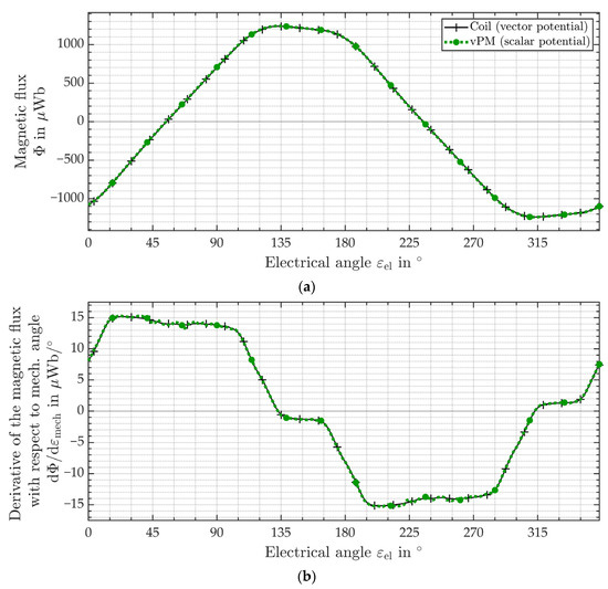
Figure 13.
Comparison of magnetic quantities of the nominal design over an electric period resulting from 2D FEA. The simulation using the magnetic vector potential (black) and current density as excitation is compared with the simulation using the magnetic scalar potential (green) and the new vPMs. In (a) the magnetic flux through coil A and in (b) the derivative of the magnetic flux through coil A with respect to the mechanical rotor angle are shown.
Since the magnetic flux through coil A is almost identical to the reference, the error of the derivative of this quantity over the mechanical rotor is also negligibly small. This is illustrated in Figure 13b. Therefore, the induced voltage in the coils is also reproduced realistically with the new approach.
4.1.3. Parameter Variation
For the nominal design of the AFM, the validity of the new approach was proven in the 2D space. However, the new approach is not limited to a specific geometry but is theoretically applicable to all magnetic actuators that have coils with soft magnetic cores. Although this work continues to focus on the AFM for validation, the input parameters of the AFM design are varied to show that the new approach is valid regardless of the specific setup.
In Table 2, the varied parameters are listed. All geometric parameters are varied by ±20%. All simulations are performed with nonlinear material behavior of the soft magnetic components, as this better describes reality. Nevertheless, one additional simulation for linear material behavior and the nominal design is performed to show the validity of the new approach for this case as well. The results of the parameter variation study are given in Table 2. The same resulting quantities are investigated as in the previous subsection, i.e., the torque, the magnetic flux through coil A, and the derivative of this magnetic flux with respect to the mechanical rotor angle. To evaluate the deviation of these quantities between the two approaches, the normalized mean absolute error is used. The normalization is performed using the value range of the respective quantity from the reference approach. The normalized mean absolute error is given in percent and allows the comparison of the results.
Table 2.
Normalized mean absolute errors of the resulting quantities for input variation in 2D FEA.
All error values in Table 2 are below 1% and most of the errors are below 0.1%, which indicates the robustness of the new approach against the variation in the basic setup of the AFM. The largest error occurs for the torque with linear material behavior of the soft magnetic components. One possible reason for this increased error is the missing saturation at singular points of sharp edges, leading to a greater impact of the edges on the torque calculation. So, this effect occurs mainly because the error values given in the table include the numerical errors. Consequently, the actual method-based errors are below the specified values.
The largest error of the parameter variation study occurs for an increment of the current density by 400% replicating current overload. In this case, the effect of the current on the magnetic field distribution is increased, thereby increasing the influence of the new approach. The magnitude of this error suggests that for current overload methodological errors of the new approach are included in addition to numerical errors. Nevertheless, the total error in this extreme case is still below 1%, so overall there is good agreement between the new approach and the reference.
4.2. 3D Simulations
For the 3D FEA, the nominal design of the AFM from Section 3 is used. The simulation space and the setup of the new approach with integrated vPMs are illustrated in Figure 14. The setup and the directional relations are similar to the 2D space. Consequently, to derive the direction of the remanent flux density or the coercivity of the vPMs based on the current directions, the right-hand rule continues to be valid. However, whereas in two dimensions the vPM zone is an area, in 3D space the vPMs occupy the whole volume of the soft magnetic core over the total axial length of the coil.
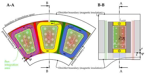
Figure 14.
Simulation space and setup of 3D FEA with vPMs replacing the three phase coils.
Moreover, Figure 14 also indicates the setup of the reference simulation with magnetic vector potential and induced current densities. In this case, unlike the simulation of the new approach, the vPMs shown in the figure are neglected and modeled as a soft magnetic core instead. In addition, the coils are modeled as homogenized multi-turn coils, which induce external current densities into the simulation.
Another difference between the setup of the 2D and 3D geometries emerges at the radial ends of the stator segments. For the 3D model of the AFM, the end windings are located between the inner and outer radius of the active zone, thereby maximizing the active air gap area compared to the resulting outer dimensions of the machine, which is a common method when stator segments are made of SMC [26,27,28]. On the other hand, the cross sections of the coil cores are decreased significantly, compared to the air gap area of each stator segment, potentially leading to higher saturated coil cores. This effect is not considered in the 2D simulations because of the missing radial dimension and a potential reason for occurring deviations between the simulations in 2D and 3D space.
Regarding the mesh quality, as mentioned above, the convergence of the analyzed quantities from the previous subsections is substantially more difficult to reach in 3D space. The moderate increase in the number of mesh nodes shown in Figure 11 leads to a significant increase in mesh nodes in the 3D space exceeding memory capacity. Therefore, a normal mesh detail with sharp edges and a moderate edge refinement is used. Hence, the numerical error is not negligible when comparing the resulting torque of both approaches.
Two simulations are performed. The first focuses on the flux calculation for the total electrical period with lower mesh refinement. The second focuses on an accurate torque calculation with higher mesh refinement over a shortened interval.
4.2.1. 3D Simulation for the Evaluation of the Magnetic Field
The resulting curves from the first simulation consist of 36 data points each and are illustrated in Figure 15. The flux through coil A, which is plotted in Figure 15a, is calculated by an integral over the flux integration area, marked in Figure 14. The derivative of this flux with respect to the mechanical rotor angle, which is plotted in Figure 15b, is calculated with the symmetric difference quotient. Similar to the 2D simulation, for both quantities from Figure 15, the curves of the new approach directly cover the reference curves. Consequently, the new approach realistically reproduces the magnetic conditions and the magnetic feedback in the 3D setup of the AFM as well.
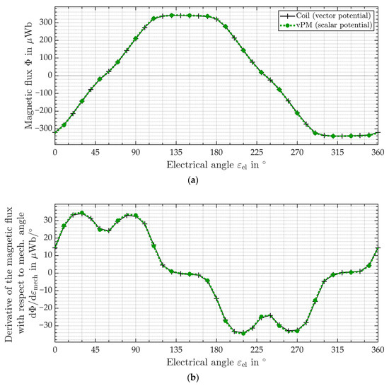
Figure 15.
Comparison of magnetic quantities of the nominal design over an electric period resulting from 3D FEA. The simulation using the magnetic vector potential (black) and current density as excitation is compared with the simulation using the magnetic scalar potential (green) and the new vPMs. In (a) the magnetic flux through coil A and in (b) the derivative of the magnetic flux through coil A with respect to the mechanical rotor angle are shown.
The quantities shown in Figure 15 present a qualitatively very similar shape compared to the 2D simulation, but their values are significantly smaller. This can be explained by the difference in the geometrical structure of the end windings between the 2D and 3D setup, which is described above. The cross-sectional areas of the coil cores in the 3D simulation are significantly smaller as a result. The reduction in the area itself but also the increased saturation lead to a decreased flux and decreased change in flux.
Referring to the computation time of this first 3D simulation, the mesh consists approximately of 1.5 million elements depending on the exact geometry for one step. This leads to approximately 2.0 million DOF for the vector potential. For the scalar potential, COMSOL solves for around 250 thousand DOF. The simulations are computed on a PC with an AMD Ryzen 9 5900X 12-Core Processor with a base frequency of 3.7 GHz and 128 GB of random-access memory (RAM). On this hardware, the simulation of one position takes 1500 s for the vector and 100 s for the scalar potential, which corresponds to an acceleration by a factor of 15. Thus, the potential to reduce simulation time was clearly demonstrated.
4.2.2. 3D Simulation for the Evaluation of the Resulting Torque
Finally, the resulting torque is investigated with the second 3D simulation. In this case, only one-sixth of the electrical period is computed, because the torque curve from the 2D simulations in Figure 12 indicates a repeating pattern every 60° (electrical). Due to its superior performance in the 2D space, the Arkkio method is used to calculate the torque. Transformed to the 3D space and into cylindrical coordinates the Arkkio torque
is calculated using the same variables and constants as in (19). The area integral from (19) transforms into a volume integral with the additional radial dimension and the radius is included in the integral. The radius is squared because during the transformation to cylindrical coordinates, another is included as a factor into the integral.
The results from the second simulation are visualized in Figure 16. Similar to the procedure during the mesh study, a simulation without electrical load is performed to generate an error estimate of the numerical errors for the final simulation. In particular, the maximum absolute error from the no-load simulation is used as an estimated error and indicated by error bars in Figure 16. It is assumed that the solution strategies have an equal contribution to the numerical error, which is why both approaches are each assigned half the estimated value for the error.
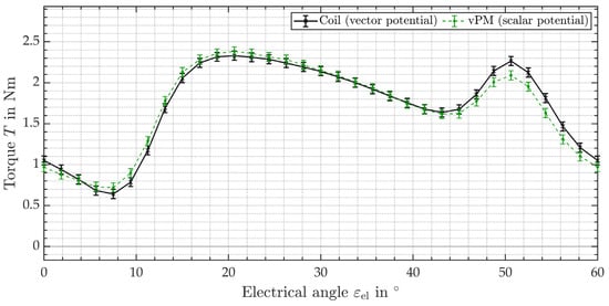
Figure 16.
Comparison of the torque (Arkkio method) of the nominal design over an electric period resulting from 3D FEA. The magnetic vector potential (black) using current density and the magnetic scalar potential (green) using the new vPMs are compared.
The resulting torque shows good agreement between both solution strategies. In contrast to the 2D simulation, the curves are not directly on top of each other, but are within the estimated numerical error for almost all data points. Only between an electrical angle of 49° and 57°, the deviation exceeds this limit. Due to an ongoing decrease in the error with increasing mesh refinement, the convergence of these torque values is not reached for the deployed mesh, but no further refinement is possible. This fact, together with the solutions from the 3D flux simulation and the 2D simulations, indicate that the numerical error is mostly responsible for this deviation. So, the new approach is a valid alternative, in 3D space as well, especially regarding the acceleration of the simulation.
For the torque calculation, the mesh consists approximately of 4.2 million elements. This leads to approximately 5.7 million DOF for the vector potential. For the scalar potential, COMSOL solves for around 720 thousand DOF. While solving for the vector potential in each step, up to 124 GB of RAM is used. The simulation of one position takes 5400 s for the vector and 200 s for the scalar potential, which corresponds to an acceleration by a factor of 27.
5. Discussion
The outcomes of the mesh and torque calculation analyses, along with the 2D and 3D simulations, are examined within the individual subsections of Section 4. In both the 2D and 3D domains, the proposed method of employing vPMs to represent coils and solving for magnetic scalar potential exhibits notable concurrence with the reference simulations that employ current-carrying coils and the magnetic vector potential. The validation process endorses the practicality of implementing vPMs solely for the soft magnetic cores of the coils. This simplifying assumption significantly reduces the modeling complexity.
A parallel can be drawn between this study’s results and those found in previous research [20,21,22], which explored the use of scalar potential-based approaches extended by thin cuts to consider the MMF of electrical currents in the context of superconductors. Similarly high levels of accuracy are observed, emphasizing the validity of such extended scalar potential approaches. Because for the new approach the entire simulation space is solved with the magnetic scalar potential, the reduction in simulation time is further increased compared to [20,21,22].
Moreover, deeper insights into the influence of sharp edges, mesh resolution, and the torque calculation method on the simulation results emerge. As described in [35], the Arkkio method provides a more accurate torque calculation compared to the classical MST method. Nevertheless, sharp edges of soft magnetic components need high refinement to avoid singularities. Especially in the 3D space, this poses a challenge due to the high number of mesh nodes required. For a better comparison, the same mesh is used for the new approach and the reference simulation. Otherwise, the mesh resolution for the scalar potential could be further increased to achieve even higher accuracies.
Whereas the validation focuses on the AFM, the new method is generally applicable. Therefore, there are no known issues preventing the new method from being transferred to other machine types with soft magnetic cores. Especially, the FEA of other 3D flux machines like the TFM potentially can be accelerated.
Finally, a more sophisticated approach could be developed by defining vPMs, also for the insulation or the air zones in the inner volume of the coil and in the coil windings so that Ampère’s law (16) is valid for these regions as well. Hence, the effect of the current density would be described more accurately in these regions. Finally, with such a revised approach, it should also be possible to realistically model air coils as well.
6. Conclusions
In this work, a new approach to accelerating multi-static 3D FEA of EMs is presented. The homogenized multi-turn coils of the EM are replaced by a vPM at the core of the coil which introduces a variable and spatially distributed MMF similar to the coils. With these vPMs replacing the current densities in the simulation space, Maxwell’s equations can be solved by using the magnetic scalar potential instead of the magnetic vector potential. Thereby, the DOF of the simulation are reduced substantially compared to the original approach.
An AFM is used as an example to validate the new approach by comparison to the original solving strategy. The validation is conducted in 2D and 3D space. Although in 2D space the new approach is not faster than the original approach, the lower computational cost of 2D simulations enables a comprehensive study of mesh quality and torque calculation. Therefore, numerical errors are significantly reduced and neglected for the comparison of both approaches. Due to limited computing capacity, the numerical error has a non-negligible influence on the simulation results in 3D space and thus is considered for validation.
In summary, the resulting torque and the distribution of magnetic flux of the new approach show very good agreement compared to the original approach. Especially, in 2D space, the errors are negligibly small even for the variation in the AFM buildup parameters. For the 3D space, the comparison of the output quantities shows good agreement especially when considering the estimated numerical error. Despite using the same mesh in the conducted 3D validation simulations, the new approach with the magnetic scalar potential and vPMs is at least 15 times faster than the reference simulation that employs magnetic vector potential and induced current densities. Furthermore, it is observed that a finer mesh resolution leads to higher acceleration factors. Therefore, the new approach has the potential to accelerate the research and development of 3D flux machines like the AFM in the future.
Author Contributions
Conceptualization, A.S.; methodology, A.S.; software, A.S.; validation, A.S.; formal analysis, A.S., U.P., B.K., M.S. and N.P.; investigation, A.S., M.S., B.K. and U.P.; resources, A.S. and U.P.; data curation, A.S.; writing—original draft preparation, A.S.; writing—review and editing, B.K., U.P., M.S. and N.P.; visualization, A.S.; supervision, U.P. and N.P.; project administration, A.S., U.P. and N.P.; funding acquisition, N.P. and U.P. All authors have read and agreed to the published version of the manuscript.
Funding
This research was funded by the Baden-Württemberg Ministry of Science, Research and the Arts as part of the research project “AD4-RESTORE” within the “InnovationCampus Future Mobility”.
Data Availability Statement
The simulation data presented in this study are available on request from the corresponding author.
Acknowledgments
The authors would like to thank the Baden-Württemberg Ministry of Science, Research and the Arts for the financial support of this research project.
Conflicts of Interest
The authors declare no conflict of interest. The funders had no role in the design of the study; in the collection, analyses, or interpretation of data; in the writing of the manuscript; or in the decision to publish the results.
Appendix A
The nonlinear magnetization curves for the SMC material S400b, which is used for the stator of the AFM, and the machining steel 1.0711, which is used for the rotor, are given in Figure A1.

Figure A1.
Nonlinear magnetization curves for the SMC S400b and the machining steel 1.0711.
References
- Meeker, D. Finite Element Method Magnetics: User’s Manual. Available online: https://www.femm.info/wiki/Files/files.xml?action=download&file=manual.pdf (accessed on 15 May 2023).
- Motor Design Ltd. Performance Analysis of Electric Motor Technologies for an Electric Vehicle Powertrain. 2019. Available online: https://www.motor-design.com/wp-content/uploads/Performance-Analysis-of-Electric-Motor-Technologies-for-an-Electric-Vehicle-Powertrain.pdf (accessed on 19 May 2023).
- Jung, J.-W.; Park, H.-I.; Hong, J.-P.; Lee, B.-H. A Novel Approach for 2-D Electromagnetic Field Analysis of Surface Mounted Permanent Magnet Synchronous Motor Taking Into Account Axial End Leakage Flux. IEEE Trans. Magn. 2017, 53, 1–4. [Google Scholar] [CrossRef]
- Zhang, B.; Epskamp, T.; Doppelbauer, M.; Gregor, M. A comparison of the transverse, axial and radial flux PM synchronous motors for electric vehicle. In Proceedings of the 2014 IEEE International Electric Vehicle Conference (IEVC 2014), Florence, Italy, 17–19 December 2014; IEEE: Piscataway, NJ, USA, 2014; pp. 1–6, ISBN 978-1-4799-6075-0. [Google Scholar]
- Gieras, J.F.; Wang, R.-J.; Kamper, M.J. Axial Flux Permanent Magnet Brushless Machines, 2nd ed.; Springer: New York, NY, USA, 2008; ISBN 1402069936. [Google Scholar]
- Kaiser, B.; Parspour, N. Transverse Flux Machine—A Review. IEEE Access 2022, 10, 18395–18419. [Google Scholar] [CrossRef]
- Chan, T.F.; Wang, W.; Lai, L.L. Performance of an Axial-Flux Permanent Magnet Synchronous Generator From 3-D Finite-Element Analysis. IEEE Trans. Energy Convers. 2010, 25, 669–676. [Google Scholar] [CrossRef]
- COMSOL AB. AC/DC Module User’s Guide: Version 6.0. Available online: https://doc.comsol.com/6.0/doc/com.comsol.help.acdc/ACDCModuleUsersGuide.pdf (accessed on 19 May 2023).
- Vanoost, D.; De Gersem, H.; Peuteman, J.; Gielen, G.; Pissoort, D. Finite-element discretisation of the eddy-current term in a 2D solver for radially symmetric models. Int. J. Numer. Model. 2014, 27, 505–516. [Google Scholar] [CrossRef][Green Version]
- Ansys, Inc. Module 01: Basics. Available online: https://courses.ansys.com/wp-content/uploads/2021/07/MAXW_GS_2020R2_EN_LE01.pdf (accessed on 19 May 2023).
- Heise, B. Analysis of a Fully Discrete Finite Element Method for a Nonlinear Magnetic Field Problem. SIAM J. Numer. Anal. 1994, 31, 745–759. [Google Scholar] [CrossRef]
- Müller, S.; Keller, M.; Enssle, A.; Lusiewicz, A.; Präg, P.; Maier, D.; Fischer, J.; Parspour, N. 3D-FEM Simulation of a Transverse Flux Machine Respecting Nonlinear and Anisotropic Materials. In Proceedings of the Comsol Conference 2016, Munich, Germany, 12–14 October 2016; pp. 1–6. [Google Scholar]
- Nakata, T.; Takahashi, N.; Fujiwara, K.; Muramatsu, K.; Ohashi, H.; Zhu, H.L. Practical analysis of 3-D dynamic nonlinear magnetic field using time-periodic finite element method. IEEE Trans. Magn. 1995, 31, 1416–1419. [Google Scholar] [CrossRef][Green Version]
- Chauhan, A. 3D Modeling of Movements in Electrical Machines Using Edge Finite Elements. Ph.D. Dissertation, Universite Grenoble Alpes, Grenoble, France, 2021. [Google Scholar]
- Stokes, A. Noncovariant gauge fixing in the quantum Dirac field theory of atoms and molecules. Phys. Rev. A 2012, 86, 012511. [Google Scholar] [CrossRef]
- Jackson, J.D. From Lorenz to Coulomb and other explicit gauge transformations. Am. J. Phys. 2002, 70, 917–928. [Google Scholar] [CrossRef]
- Ansys, Inc. Module 02: Quasitatic Solvers. Available online: https://courses.ansys.com/wp-content/uploads/2021/07/MAXW_GS_2020R2_EN_LE02.pdf (accessed on 19 May 2023).
- Ferrario, A. How to Model Rotating Machinery in 3D. Available online: https://www.comsol.com/blogs/how-to-model-rotating-machinery-in-3d/ (accessed on 19 May 2023).
- Griesmer, F. Quick Intro to Permanent Magnet Modeling. Available online: https://www.comsol.com/blogs/quick-intro-permanent-magnet-modeling/ (accessed on 19 May 2023).
- Shen, B.; Grilli, F.; Coombs, T. Overview of H-Formulation: A Versatile Tool for Modeling Electromagnetics in High-Temperature Superconductor Applications. IEEE Access 2020, 8, 100403–100414. [Google Scholar] [CrossRef]
- Arsenault, A.; Alves, B.d.S.; Sirois, F. COMSOL Implementation of the H-ϕ-Formulation With Thin Cuts for Modeling Superconductors With Transport Currents. IEEE Trans. Appl. Supercond. 2021, 31, 1–9. [Google Scholar] [CrossRef]
- Arsenault, A.; Sirois, F.; Grilli, F. Implementation of the H-ϕ-Formulation in COMSOL Multiphysics for Simulating the Magnetization of Bulk Superconductors and Comparison With the H-Formulation. IEEE Trans. Appl. Supercond. 2021, 31, 1–11. [Google Scholar] [CrossRef]
- Paudel, N. Guidelines for Modeling Rotating Machines in 3D. Available online: https://www.comsol.com/blogs/guidelines-for-modeling-rotating-machines-in-3d/ (accessed on 19 May 2023).
- Vansompel, H.; Leijnen, P.; Sergeant, P. Multiphysics Analysis of a Stator Construction Method in Yokeless and Segmented Armature Axial Flux PM Machines. IEEE Trans. Energy Convers. 2019, 34, 139–146. [Google Scholar] [CrossRef]
- Le, W.; Lin, M.; Lin, K.; Liu, K.; Jia, L.; Yang, A.; Wang, S. A Novel Stator Cooling Structure for Yokeless and Segmented Armature Axial Flux Machine with Heat Pipe. Energies 2021, 14, 5717. [Google Scholar] [CrossRef]
- Echle, A.; Pecha, U.; Parspour, N.; Gruner, C. Design of a Novel High Power Density Single Sided Axial Flux Motor Using SMC Materials. In Proceedings of the 2020 International Conference on Electrical Machines (ICEM), Gothenburg, Sweden, 23–26 August 2020; IEEE: Piscataway, NJ, USA, 2020. ISBN 9781728199450. [Google Scholar]
- Winterborne, D.; Stannard, N.; Sjoberg, L.; Atkinson, G. An Air-Cooled YASA Motor for in-Wheel Electric Vehicle Applications. IEEE Trans. Ind. Appl. 2020, 56, 6448–6455. [Google Scholar] [CrossRef]
- Zhang, B.; Seidler, T.; Dierken, R.; Doppelbauer, M. Development of a Yokeless and Segmented Armature Axial Flux Machine. IEEE Trans. Ind. Electron. 2015, 63, 2062–2071. [Google Scholar] [CrossRef]
- COMSOL AB. COMSOL Multiphysics® Version 6.1; COMSOL AB: Stockholm, Sweden, 2022. [Google Scholar]
- Egea, A.; Almandoz, G.; Poza, J.; Gonzalez, A. Axial flux machines modelling with the combination of 2D FEM and analytic tools. In Proceedings of the XIX International Conference on Electrical Machines–ICEM 2010, Rome, Italy, 6–8 September 2010; IEEE: Piscataway, NJ, USA, 2010; pp. 1–6, ISBN 978-1-4244-4174-7. [Google Scholar]
- Niemimäki, O.; Kurz, S. Quasi 3D modelling and simulation of axial flux machines. COMPEL: The International J. Comput. Math. Electr. Electron. Eng. 2014, 33, 1220–1232. [Google Scholar] [CrossRef]
- Jin, J.-M. Theory and Computation of Electromagnetic Fields; Wiley: Hoboken, NJ, USA, 2010; ISBN 9780470874257. [Google Scholar]
- Arkkio, A. Analysis of Induction Motors Based on the Numerical Solution of the Magnetic Field and Circuit Equations; Helsinki University of Technology: Otaniemi, Finland, 1987; ISBN 951-666-250-1. [Google Scholar]
- COMSOL AB. Permanent Magnet Motor in 3D. Available online: https://www.comsol.de/model/download/1032561/models.acdc.pm_motor_3d.pdf (accessed on 19 May 2023).
- Silwal, B.; Rasilo, P.; Perkkio, L.; Oksman, M.; Hannukainen, A.; Eirola, T.; Arkkio, A. Computation of Torque of an Electrical Machine With Different Types of Finite Element Mesh in the Air Gap. IEEE Trans. Magn. 2014, 50, 1–9. [Google Scholar] [CrossRef]
Disclaimer/Publisher’s Note: The statements, opinions and data contained in all publications are solely those of the individual author(s) and contributor(s) and not of MDPI and/or the editor(s). MDPI and/or the editor(s) disclaim responsibility for any injury to people or property resulting from any ideas, methods, instructions or products referred to in the content. |
© 2023 by the authors. Licensee MDPI, Basel, Switzerland. This article is an open access article distributed under the terms and conditions of the Creative Commons Attribution (CC BY) license (https://creativecommons.org/licenses/by/4.0/).