Iron Loss Calculation Methods for Numerical Analysis of 3D-Printed Rotating Machines: A Review

Abstract

Three-dimensional printing is a promising technology that offers increased freedom to create topologically optimised electrical machine designs with a much smaller layer thickness achievable with the current, laminated steel-sheet-based technology. These composite materials have promising magnetic behaviour, which can be competitive with the current magnetic materials. Accurately calculating the iron losses is challenging due to magnetic steels’ highly nonlinear hysteretic behaviour. Many numerical methodologies have been developed and applied in FEM-based simulations from the first introduced Steinmetz formulae. However, these old curve-fitting-based iron loss models are still actively used in modern finite-element solvers due to their simplicity and high computational demand for more-accurate mathematical methods, such as Preisach- or Jiles–Atherton-model-based calculations. In the case of 3D-printed electrical machines, where the printed material can have a strongly anisotropic behaviour and it is hard to define a standardised measurement, the applicability of the curve-fitting-based iron loss methodologies is limited. The following paper proposes an overview of the current problems and solutions for iron loss calculation and measurement methodologies and discusses their applicability in designing and optimising 3D-printed electrical machines.

1. Introduction

The additive manufacturing of Soft Magnetic Materials (SMMs) is an increasingly important area [1,2,3,4,5]. Within this area, the design of layered composite structures made from multiple materials has given rise to a new research field that draws parallels between laminated steel sheet cores and 3D-printed layered structures [6,7,8,9]. The following sections will refer to these materials as Soft Magnetic Layered Composites (SMLCs). The term layered structure typically refers to an alternating metal and electrically insulating material arrangement. In this paper, this terminology discusses two-component systems, but the simultaneous use of three or more materials can also occur. This technology offers exceptional design freedom, fast prototyping, and reduced material waste. For electrical machines, additive manufacturing allows designs with optimised mechanical, electromagnetic, and thermal parameters [10,11,12]. The proliferation of electrically powered vehicles and the limited availability of rare-earth metals demand new, advanced solutions from today’s engineers [13,14]. Traditionally, iron cores for electrical machines are made from laminated steel sheets or Soft Magnetic Composites (SMCs) [15,16,17]. For iron cores, important physical characteristics are saturation magnetisation ($B_s$), intrinsic coercivity ($H_c$), remanent magnetic field ($B_r$), relative permeability (${\mu }_r$), hysteresis loss density ($P_h$), eddy current loss ($P_e$), DC bias, and yield strength. Some of the previously mentioned characteristic quantities are depicted in Figure 1 for the case of the FeCo material. Magnetic permeability describes the strongly nonlinear connection between the magnetic field and these ferromagnetic materials. Moreover, this hysteresis curve’s shape can strongly depend on the frequency of the alternating magnetic field [18]. Figure 1 also compares the hysteresis characteristics of different 3D-printed materials, a FeCo, a FeNi, and a FeSi alloy, to an M270-50A grade, laminated steel sheet, which is a widely used material in electrical machines. The FeCo alloy has the widest hysteresis curve, which means that this material has the highest iron losses. In the case of the M270 material, there is no stress nor structural anisotropy. The FeSi material’s characteristics make it the best competitor with the M270 material. A heat treatment can improve the 3D-printed material’s parameters. However, this picture shows their current built-in state.

On the other hand, soft magnetic composites are suitable for forming spatial flux paths. In many cases, these can be created during the pressing process without mechanical machining so that the properties of the finished product and the starting material are similar. An additional advantage of these materials is that eddy current losses are lower, even at higher excitation frequencies than for laminated cores. However, in addition to the numerous advantages, there are disadvantages in using SMCs, with higher hysteresis losses and intrinsic coercivity than laminated iron cores and a lower relative permeability and yield strength [19]. The production of magnetic materials by metal 3D printing opens up the possibility of creating complex geometries from alloys that are difficult or impossible to machine by other methods (high-silicon steel [20,21,22], amorphous [23,24,25]).

Figure 1. Comparing the hysteresis loops of 3D-printed toroid cores from FeCo, FeNi, and FeSi alloys with a conventional M270-50A material [26,27].

Figure 1. Comparing the hysteresis loops of 3D-printed toroid cores from FeCo, FeNi, and FeSi alloys with a conventional M270-50A material [26,27].

In the case of laminated iron cores, mechanical and thermal treatments can significantly change the magnetic properties of the laminated structure compared to the starting material [28]. Besides the significant amount of waste generated during lamination, another major problem with this technique is that the design of 3D flux paths is not feasible or can only be achieved by very complex manufacturing techniques. A plate thickness of a few tenths of a millimetre is common for classically produced laminated iron cores. They are fixed together by mechanical sheet forming or welding. The additive manufacturing (AM) process typically builds up the 3D part from layers of a few tens of micrometres. The layers are often fused together. In the latter case, the lower limit for the thickness of the laminated layers is always determined by the layer thickness used [29].

This paper briefly overviews the possibilities and current problems with the 3D printing of soft magnetic materials as an iron core. The paper can be divided into two main parts, where the first part of the paper shows a current overview of the leading 3D printing technologies and the brittleness and applicability of FeSi materials in 3D-printed electrical machines. The second part overviews the iron loss calculation methodologies. Most of the proposed numerical methods can be used to model the iron losses in 3D-printed materials. These methods differ not only in their accuracy and computational demand, but they can require different complexities in measurements to determine the material-dependent parameters, as well. Moreover, the accuracy of the applied formula can depend on the type of examined material. Some of the presented formulas can be easily applied to calculate ferrite cores, but other formulas have better results for grain-oriented materials [30].

The paper shows the main applicable formulas with their advantages and disadvantages. After introducing the calculation examples, a classical and a dynamical Preisach-model-based iron loss approach are presented in a theoretical example. This profound explanation and practical example aim to help the reader select the appropriate measurement and numerical formula for the iron loss calculation task.

2. Advancements of 3D Printing Technology

Additive engineering of soft magnetic layered composites can result in structures with different microstructures and compositions. The selection of the appropriate printing technology (see Figure 2), the geometric design [31,32,33], and the variation of the process parameters and raw materials during printing [24,34,35] all offer the possibility to achieve tailored microstructures, domain structures, and magnetic properties. The fundamental goal of designing a composite structure is to reduce the magnitude of the eddy current induced in the ferromagnetic part to increase the operating frequency range, ultimately leading to the miniaturisation of our electrical equipment. If we can reduce the dissipative losses, we can improve the energy balance of our equipment by omitting cooling or reducing power. From the relation between the energy stored in the coil (where L is the inductance, $I_{max}$ is the maximum current flowing in the coil) and the energy stored in the magnetic field (where ${\mu }_0$ is the vacuum permittivity), we can observe the following relation between the effective permeability and volume:

$$\frac{{\mu }_{eff}}{V}=\frac{B_{max}^2}{{\mu }_0{I}_{max}^{2}L},$$

(1)

which gives the maximum saturation of the magnetisation ($B_{max}$) for the maximal effective permeability (${\mu }_{eff}$) and the minimal magnetised volume (V).

The different additive technologies allow the creation of different composites [36,37,38,39]. Depending on the energy source used, it is possible to form (print) the structural integrity of metals, ceramics, or polymers in the desired shape. Typically, a single apparatus can be used to deposit, melt, or cross-link a group of materials. The vast majority of studies [36,40,41,42,43] are focused on soft magnetic composites with organic insulators using simpler technologies. Here, we focused on solutions for the design of metal–ceramic composites. These research works are mainly relevant for devices capable of operating effectively in higher frequency and temperature ranges. In most cases, the printing technology used determines the composite structure that is practical or possible to produce. Based on Figure 2, Wire Direct Energy Deposition (Wire-DED), Powder Direct Energy Deposition (Powder-DED), Selective Laser Melting (SLM), and Electron Beam Melting (EBM) technologies are suitable for the formation of laminated metal–insulator composites. Of these, Powder-DED, SLM, and EBM are of practical importance. Core–shell structured SMCs can be realised by Powder-DED, SLM, EBM, Binder Jetting (BJ), and Bound Powder Extrusion (BPE) technologies [44,45,46].

The Wire-DED technology melts metal wires together with arc welding, quickly resulting in a preform similar to the net-shape model. The available materials are very similar to those used for welding. However, the combination of different material groups is still unresolved. The Powder-DED technology can already combine different materials or even produce metal alloys by combining elemental metal powders. At the end of printing, we obtain a near-final product. In many cases, only the machining of the fitting and contact surfaces is necessary. SLM allows the use of pre-alloyed powders. The technology is not among the fastest processes, but its support-free printing is also available on the market. In some cases, multi-material printing is also possible. The internal stress state following the cooling is a major problem in each case. Multi-material printing significantly increases the occurrence of delamination and microcracks, which can lead to the complete failure of the printing. The stress state can be reduced during the printing process by systems supplemented with thermal imaging cameras, which can correct parameter settings layer-by-layer, or it is also possible to use a stress-relieving heat treatment post-process.

The typical soft magnetic properties of additively manufactured structures and those of powder cores and laminated structures produced by classical manufacturing techniques differ in many ways. In addition to the internal coercivity, the static permeability and cut-off frequency values can qualify the softness of core–shell and laminated structures during measurements. The cut-off frequency can be calculated from Snoek’s law [47]. The cut-off frequency is where the real part of the complex permeability changes significantly. Figure 3 summarises the characteristic values for the two types.

The coercive field of soft magnets increases with decreasing grain size. A size-dependent demagnetisation factor explains the grain size dependence of coercivity. Mager gave the phenomenological description [48] in the form of a linear relation between the coercive field and the reciprocal of the grain size (1/GS), in which the slope is proportional to the ratio of the domain wall surface energy ($\gamma$) to saturation polarisation ($J_s$). The effect of the grain size is evident for the AM SMLC and powder cores. For layered structures, the detrimental effect of surface pining should be considered. Considering the effectiveness of these effects, we prepared the soft magnetic parameters ($H_c$, ${\mu }_{static}$, and $f_{lim}$) evaluation table presented in Figure 3. The dominance of eddy currents determines the limitation of the cut-off frequency. By reducing the layer thickness and preventing the formation of a large current path, it is possible to extend the operational frequency range. In the design of the composite structure, particular emphasis should be placed on the choice of the filling factor. The insulating of core–shell materials as a grain significantly increases the proportion of the insulating phase in the structure, which deteriorates the macroscopic magnetic properties of the material (e.g., $B_s$). Forming a coherent, damage-free insulating layer with a few micrometres of thickness is not feasible in 3D printing to obtain a quasi-porosity-free, mechanically sound structure after printing. In contrast, a layered design allows the deposition of a certain thickness of the insulating layer per predefined number of layers. The appropriate parameters for each type of material guarantee the printing of a quasi-compact structure. Due to the cyclic thermal stresses during production and the typically low thermal shock resistance of ceramics, it is advisable to minimise the metal–ceramic contact surfaces and to combine material pairs with nearly identical thermal expansion coefficients [35]. In addition, it is essential to note that the mechanical properties (except compressive strength) of ceramic layers are far below those of pure metallic structures [6,35,49,50].

It is also important to mention the possibility of using additively manufactured SMC iron cores with a sinterless powder or air layer for electrical insulation [6,21]. In these cases, the ferromagnetic filling factor could be better since a continuous air layer can only be formed by not sintering several layers, resulting in an insulating layer with a thickness of several hundred micrometres [21]. The dust particles trapped in the air gap create electrical percolation paths between the layers, which increases eddy current losses. An advantage, however, is that there is only a single base material, so there is no mixing of two powders with different compositions during the printing process of the layered structure. From an economic point of view, it is significant that the subsequent separation of different raw materials is often not feasible or only very costly [51]. It is important to note that one of the most-expensive components of powder additive technologies is currently the gas-phase powder raw material.

Regarding technological implementation, the Wire-DED process has yet to show practical relevance for producing metal–ceramic composites. In the Powder-DED and EBM processes, it is relatively easy to alternate metallic and ceramic materials by employing a suitable adjustment of the powder dosage and the applied energy density [52,53,54,55,56,57,58,59,60,61,62,63]. In the SLM process, the applied laser wavelength differs by three orders of magnitude for metallic and ceramic materials. A dual-laser system can be used for printing, including a laser with a wavelength of 1 $\mathsf{\mu }$m for melting metallic material and a laser with a wavelength of 1 mm for ceramics. However, this problem can be eliminated by, for example, in situ oxidation during printing, nitriding, carbonisation, or possible post-printing annealing processes [24]. There are ceramics with absorption coefficients close to those of certain metallic materials, so direct metal–ceramic composite printing cannot be ruled out [34,50]. Printing the metal–metal structure and its subsequent post-process modification (nitriding, carbonisation, oxidation) can promote better interfacial contact between the two base metals and result in defect-free microstructures and macrostructures.

In many ways, additively manufactured iron core geometries offer engineers new design perspectives. It is also important to note that most metal 3D printing technologies impart a unique microstructure to the printed structure. In the case of SLM technology, a part built layer-by-layer in the Z direction on a table plate placed in the XY plane develops columnar grains parallel to the Z axis [22,64]. For sheet metal bodies, it is feasible to have the magnetic flux lines and the columnar grain structure of the metal plate coincide, which is half of the easy magnetisation direction for silicon steels. On a theoretical plane, in the case of toroidal iron cores, it would be possible to distort the crystal structure along the circumferential arc to a certain extent. Oliveira et al. investigated the build orientation effect on the magnetic properties of managing steel 300. They concluded that there is likely a correlation between the residual stresses and coercivity, remanence. The ring-like specimens’ printing orientation were XYZ, XYZ-45°, and YZX. Figure 4 shows the magnetisation curves and hysteresis loops of these samples. M. Garibaldi et al. examined the grain orientation and structure for different print orientations, which are illustrated in Figure 5, for Fe-6.5wt %Si composition.

The raw materials most-commonly used in producing additively manufactured iron cores are the same as those used in the classical production of components. There are several kinds of research works on macroscopic sintering of amorphous and partially crystalline alloys, which have been popular since the 1980s [23,66,67,68,69]. The difficulty of the realisation is that rapid cooling is not possible, as the melting and sintering of new layers is cyclically performed during the printing process. The possibility of rapid cooling may still work for the first layers, but the internal stresses that freeze can cause significant mechanical and magnetic degradation during subsequent use. With expensive nucleation inhibitors and nucleation-inhibiting or stimulating alloying agents, a specific size range can be achieved, resulting in an amorphous/partially crystalline structure. The problems described above can be avoided using technologies such as Fused Filament Fabrication (FFF = BPE) [70]. In our research, we guaranteed the amorphousness and low cost of the raw material for SLM technology by using simple iron metalloids (FeC, FeB, FeSi, FeP) with significantly different atomic diameters, preventing the Short-Range Ordering principle (SRO principle) [23]. The atoms do not have time to arrange themselves in a crystalline structure due to the size difference and the thin layer application. The large-sized steel base plate on which the printing takes place has enough heat dissipation capacity to achieve quasi-rapid cooling. The 3D printability of high-saturation-magnetisation Fe₃₅Co₆₅ or the extremely soft Fe₂₀Ni₈₀ alloy, known under the Permalloy brand name, is a relatively easy task since standard steel powders often contain significant amounts of Co and Ni in addition to Fe [64,71,72,73]. The printability of Fe-Si alloys becomes problematic somewhere around 6.5wt% silicon [74]. The presence of high amounts of silicon causes the material to become extremely brittle, which can easily crack due to cyclic thermal stress and internal stresses during printing. By reducing the difference between the sintering and table temperatures, i.e., by significantly increasing the table temperature, microstructural defects can be somewhat eliminated, and large complex geometries can be formed from this material. In addition, process parameters such as laser power, scanning speed, focal point diameter, and scanning strategy all impact the resulting macrostructure and its magnetic properties [75,76].

There are several kinds of research on the printability of Fe-6.5wt%Si with zero magnetostriction, which is a comparatively inexpensive material, but has relatively good soft magnetic properties [9,22,38,76]. The porosity values for pre-alloyed specimens made of gas-atomised powder were investigated for different values of volumetric energy density. M. Garibaldi et al. investigated the effect of the laser printing parameters on the microstructure and crack formation. It has been shown that irregularly shaped porosities typically form at the interfaces of shallow and wide melt pools, while spherical pores form at the bottom of deeper melt pools. They also proved that the cumulative crack length (c.c.l.) parameter starts to increase significantly above an energy input of 280 J/m. However, large, irregularly shaped pores can also be eliminated from the microstructure in the case of an energy input of 280 J/m. These results are shown in Figure 6.

A solution to avoid structural defects and high brittleness is the development of a gradient composition, which can be obtained by appropriate layering and laser sintering of elemental iron and silicon powders. In this case, the ideal alloying amount of 6.5wt%Si will be present only in a certain cross-section, with more or less silicon being observed elsewhere. The cross-sectional gradient changes of the elemental composition are shown in [26]. The CT porosity measurements and scanning electron microscopy sectional view of such a sample is illustrated in Figure 7.

3. Measurement Methodologies for Iron Losses

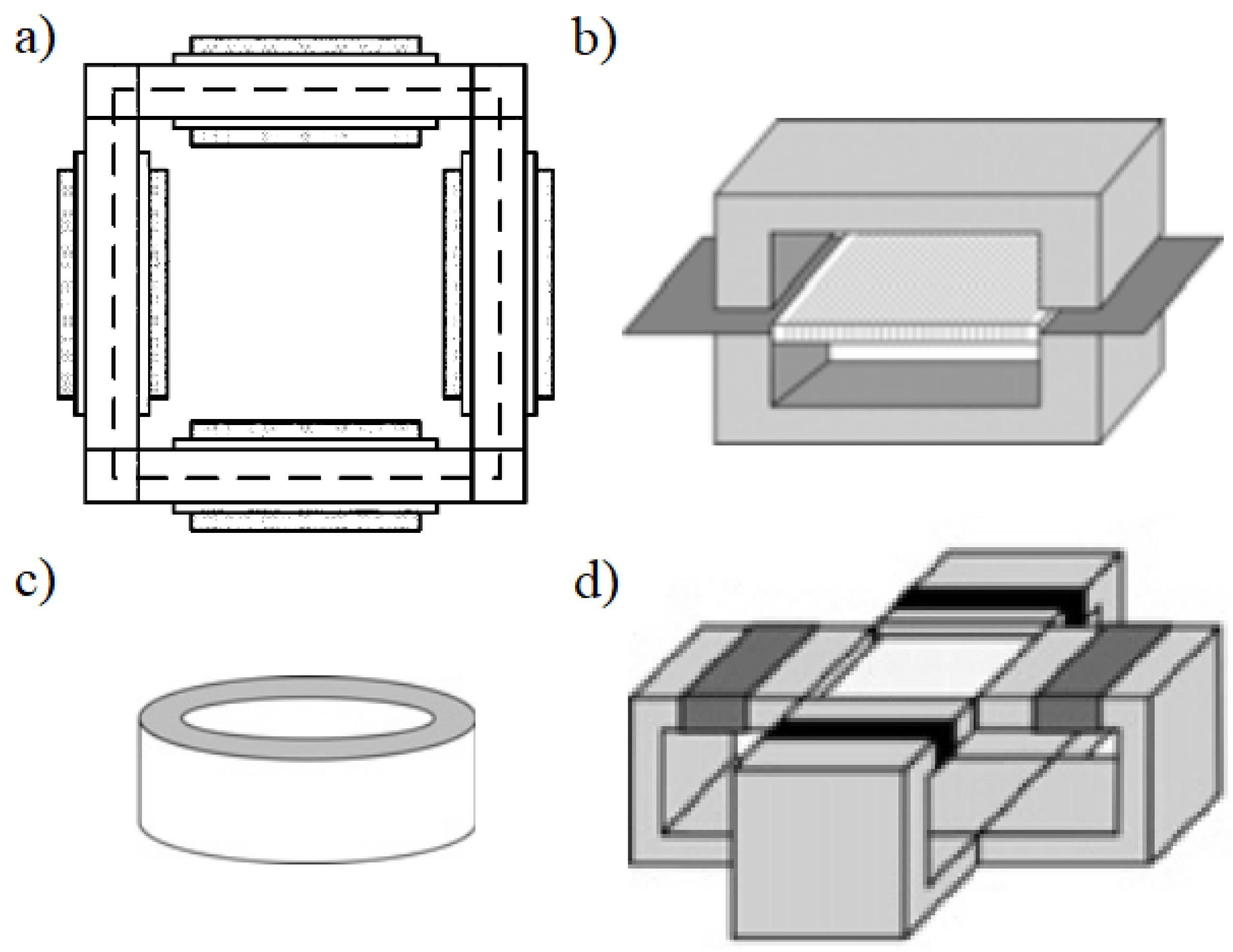
When measuring the magnetic properties of 3D-printed parts, it is important to remember that the manufacturing technology, the geometry of the printed part, its location in the printing space, and its material composition all influence the selection of the appropriate measurement method. In the measurement technique of 3D-printed structures, we must distinguish between the measurement of sheet metal and complex geometries (toroid, stator, rotor, etc.). The relationship between printing and measurement parameters must be taken into account in all cases. In classic manufacturing processes, such as rolling Fe-Si sheets, both oriented and non-oriented grain structures can be formed. A similar situation exists for 3D-printed materials, with the difference that, in the case of PBF technologies, a dendritic grain structure forms in the direction of layer-by-layer construction (referred to as the direction along the Z axis). It is, therefore, easy to understand that, in the case of the 3D printing of sheet specimens, a permanent grain orientation can be established, which, under appropriate measurement setup, aligns with the direction of magnetic flux. Further parallels can be drawn between the cutting techniques for sheets (such as stamping, punching, abrasive or laser cutting, wire electric discharge machining) and laser sintering, as the microstructure and domain structure that form in both cases can often be modified, made unique through the appropriate selection of the cutting parameters and laser scanning strategy.

There are several standardised methods for the measurement of laminated iron cores. These standards precisely define the measurement conditions, the shape and physical dimensions of the sample, as well as the parameters of the instruments required for the measurement. The IEC standards [77,78,79] distinguish three different measurement methods based on the shape of the measured sample. These are the so-called Epstein frame, single-sheet, and toroidal core measurement methods [80]. In the case of 3D-printed iron cores, there are no standardised measurement procedures; researchers usually use the toroidal core measurement method [81,82].

All of the measurement methods presented below are computer-controlled, and their general principle of operation is shown in Figure 8. For the measurement, a primary ($N_1$) and a secondary ($N_2$) coil need to be placed on the sample. The primary coil should be connected in series with a resistance (R) without inductance and fed with a sinusoidal voltage, while the secondary circuit should be left unloaded. This essentially creates a transformer operating in an open-circuit condition. The voltage across the resistance ($u_1$) and the voltage across the open secondary coil ($u_2$) are measured using a data acquisition card. The computer processes the voltage measurements from the data acquisition card and performs the necessary calculations. According to the standards, the tested samples need to be demagnetised before the measurement by applying an excitation that corresponds to more than ten-times the coercive field strength and gradually reducing it to zero.

Using the measured voltages $u_1$ and $u_2$, the magnetic field strength (H), magnetic induction (B), and power loss ($p_s$) can be calculated using the following equations [83]:

$$H=\frac{N_1}{R{l}_{eff}}{u}_1\left(t\right),$$

(2)

$$B=\frac{1}{N_{2}A}{\int }_0^t{u}_2\left(\tau \right)d\tau ,$$

(3)

$$p_s=\frac{f{N}_1}{N_{2}mR}{\int }_0^T{u}_1\left(t\right)u_2\left(t\right)dt,$$

(4)

where $N_1$ is the number of turns in the primary coil, $N_2$ is the number of turns in the secondary coil, m is the mass of the sample, $l_{eff}$ is the effective length of the magnetic field, A is the cross-sectional area of the sample, R is the purely ohmic resistance, f is the excitation frequency, and $T=\frac{1}{f}$ is the period of the waveform.

3.1. Epstein Frame

In the case of the Epstein frame [84] measurement method, the laminated iron cores to be examined are arranged in a square configuration, as shown in Figure 9a. The edges of the square consist of multiple laminated iron core strips, and double-overlapping is applied at the corners so that the cross-sectional area and average length of the frame are equal on all sides of the frame. The strips used for the frame sides are cut from a rolled sheet coil to produce the iron core. The cutting direction can be the same as the rolling direction at each side of the frame. However, different cutting directions can also be chosen to measure anisotropy. Th 3D-printed iron core strips can be cut from the printed material to construct the frame [85]. Primary and secondary winding arrangements are placed on each side of the frame. The four primary and secondary windings are connected in series accordingly, forming a common primary and secondary winding. The standard defines the dimensions of the frame, the minimum weight, and the number of turns for the windings.

3.2. Single-Sheet Tester Measurement

In the case of the single-sheet tester [86] measurement method, the sample under investigation consists of a single sheet. The primary and secondary windings are placed on the sample, and two steel yokes enclose the magnetic circuit. These yokes are made of high-quality electrical steel, typically grain-oriented electrical steel or nickel-iron alloy, to minimise their influence on the measurement results. The standard defines the dimensions of the sample and the steel yokes, the magnetic properties of the steel yokes, and the number of turns for the windings. The fundamental structure and realisation of the single-sheet tester method can be seen in Figure 9b.

3.3. Toroidal Sample Measurement

The properties of magnetic materials can also be measured using toroidal samples, as shown in Figure 9c. According to international standards [79], this method is suitable for examining special alloys, nanocrystalline and amorphous materials, injection-moulded and cast materials, pressed and sintered materials, as well as soft magnetic composite materials, but not magnetic laminations. This also includes 3D-printed toroidal samples. For the measurement, toroidal samples can be created in various ways, such as using wound strips, rings cut from larger sheets, pressed powder, cutting cores from larger materials, or 3D printing toroidal cores. It is essential to mention that the measurement results depend on the sample preparation [80]. For example, windingintroduces stress in the material, which affects the magnetic parameters of the material. The primary and secondary windings are placed on the toroidal sample. For toroidal samples, the standard does not specify the exact geometrical dimensions or the number of turns in the windings; it only provides some recommendations. Moreover, this method is not suitable for measuring the magnetic properties of the material in a specific direction, thus for investigating grain-oriented cores.

3.4. Multidimensional Measurement Methods

The examined sheet is excited in one direction in the previously discussed methods. However, in the case of rotating magnetic machines, the iron core is subjected to magnetisation in multiple directions simultaneously. In addition to alternating current excitation, rotating magnetisation also occurs. The losses in the iron core vary depending on the magnitude of rotating and alternating excitations. In the case of moderate amplitudes, the losses arising from rotating magnetisation can be significantly greater. Therefore, to examine the iron core material, it may be important to conduct multidimensional analysis [87], exposing the sample to multi-directional excitations. Multidimensional analysis is also important for materials with high anisotropy, such as grain-oriented materials.

In the case of multidimensional analysis, the magnetic field is controlled using the same steel yokes as in the single-sheet measurement method. Rotating and multi-directional magnetic excitation can be generated by rotating the steel yokes or with stationary steel yokes and appropriately controlling the excitation of the windings. The arrangement in Figure 9d allows for the acquisition of the hysteresis characteristics of the sample in the x and y directions. From that, the hysteresis loss of the sample can be calculated using the following equation:

$$p=\frac{f}{\rho }{\int }_0^T\left(B_x\left(t\right)\frac{d{H}_x\left(t\right)}{dt}+B_y\left(t\right)\frac{d{H}_y\left(t\right)}{dt}\right)dt.$$

(5)

Based on the steel yoke method presented here, three-dimensional measurements can also be performed by extending Equation (5) to include the third component along the y axis.

4. Iron Loss Modelling Approaches, an Overview

Calculating the magnetic losses of electrical machines is a highly engineered task, which needs to consider many factors. The iron losses depend not only on the applied material, but the manufacturing method, as well [88,89,90].

FEM-based solvers usually use a post-processing step to calculate iron losses. In this solving step, using the calculated magnetic flux distribution values, loss values are calculated for the element using an analytical material model [91,92,93]. The accuracy of these formulae usually depends on the measurements to which the free parameters of the formula are fit. These measurements can be made on an Epstein frame, a toroidal core setup, or in a single-plate tester [91], depending on which method is best suited to the particular calculation. The following section aims to introduce these iron-loss-calculation methods and describe their applicability, besides their advantages and disadvantages.

4.1. Steinmetz-Equation-Based Formulas

The first and simplest such material model, still widely used today, is the Steinmetz formula [94], which is fit to a measurement made by a sinusoidal excitation at a given frequency. Currently, this form is extended with a frequency-dependent parameter; this formula is referred to as the Steinmetz formula or power law as well in the literature [95,96,97,98,99,100,101,102,103,104,105], and it can be written in the following form:

$$p=C_{sc}·f^{\alpha }·{\widehat{B}}^{\beta },$$

(6)

where p represents the power loss in W/m${}^3$, $\widehat{B}$ represents the peak value of the magnetic flux density in the examined material, $C_{sc}$ is the Steinmetz coefficient, and the $\alpha$ and $\beta$ coefficients are usually determined from the measurements. This formula works in a limited frequency range for sinusoidal waves and a constant or DC-biased excitation frequency [100,106].

The very first extension of this formula was the Modified Steinmetz Equation (MSE). The model assumes that this remagnetisation rate is proportional to the change of the magnetic flux density; a macroscopic re-magnetisation-based equivalent frequency ($f_{eq}$) can be introduced by the following formulae [107,108,109]:

$$f_{eq}=\frac{2}{{(B_{max}-B_{min})}^2{\pi }^2}{\int }_0^T{(\frac{dB\left(t\right)}{dt})}^{2}dt.$$

(7)

Inserting this $f_{eq}$ into Equation (6), we obtain the following form for the modified Steinmetz equation [107,108,109,110]:

$$p=C_{sc}·f_{eq}^{\alpha -1}·{\widehat{B}}^{\beta }·f_r,$$

(8)

where $f_r$ is the remagnetisation frequency, and the other parameters $C_{sc}$$\alpha$ and $\beta$ are the same as introduced in (6). With an application of a second correction factor, this formula can also handle the DC bias premagnetisation; however, this formula is not accurate when the exciting wave fundamental frequency is relatively small, and this formula is not internally consistent [106,109,110].

Another approach, the generalised Steinmetz equation, considers the rate of magnetic induction change and depends on its instantaneous value. This formula is consistent, but does not fit well with the measurements if the third or higher harmonic part of the formula becomes significant; thus, it can result in multiple peaks in the resulting waveforms [99,106,110]. The improved generalised Steinmetz equation resolves these problems with the multiple waveforms [95,111], dividing the flux density waveforms into major and minor loops and calculating the iron losses separately in the following form:

$$p=\frac{1}{T}{\int }_0^T{C}_{SE}|\frac{dB}{dt}{|}^{\alpha }{|\Delta B|}^{\beta -\alpha }dt,$$

(9)

where $\Delta B$ defines the peak-to-peak flux density of the minor and major loops of the current waveform. Applying $\Delta B$ instead of B(t) resolves the DC bias sensitivity problem [95,110]. Another method, the natural Steinmetz equation, uses a similar change of the time-dependent flux density ($B\left(t\right)$) value with $\Delta B$ [104] to improve the performance of the approximation in a different way:

$$p={(\frac{\Delta B}{2})}^{\beta -\alpha }\frac{C_{SE}}{T}{\int }_0^T{|\frac{dB}{dt}|}^{\alpha }dt;$$

(10)

however, in this approach, the waveform of the excitation is not divided into minor and major loops. It is directly applied to the whole period. In [103], a similar, but simple approach was published with the name waveform coefficient Steinmetz equation. Other newer approaches such as the dual-natural Steinmetz equation use the combination of two iGSE methods, one to model the hysteresis and a second one to model the dynamic losses [112,113].

These Steinmetz-formula-based approaches offer a simple and fast way to predict iron loss without deep knowledge and without measurements of the materials. The weakness of these formulas is that the Steinmetz coefficients should vary with the applied frequency. This results in the accuracy of these formulas being lower than other mathematical-description-based methodologies, such as the Preisach or Jiles–Atherton method, especially at lower frequencies, where the losses mainly depend on the effect of the hysteresis. The rotational losses are also not considered by the previously mentioned formulas [106,109,111].

4.2. Separation of the Losses

The other type of function approximation models is based on the loss separation methodology. The first approach was introduced by Jordan in 1924 [114]. In this approach, the hysteresis and eddy-current-based losses (also called dynamic losses) are modelled separately. The model assumes that the hysteresis losses are caused by irreversible magnetisation effects (Brakhausen jumps) [115,116], while the dynamic losses are related to the generation of the eddy current near the domain walls:

$$P=P_{hyst}+P_d=C_{h}f{B}^2+C_d{f}^2{B}^2,$$

(11)

where $P_{hyst}$ means the hysteresis losses, $P_d$ represents the dynamic eddy current losses, while the $C_h$ and $C_e$ parameters can be determined from a measurement. The model expects that the hysteresis losses at low frequencies mainly cause the losses. The eddy current losses can be calculated in a laminated thin sheet, and it can be written in the following form [109,117]:

$$P_{ec}=\frac{\sigma d^2}{12\rho }{\left(\frac{dB\left(t\right)}{dt}\right)}^2,$$

(12)

The eddy current loss term can be derived from Maxwell’s equations, where d is the lamination thickness, $\rho$ is the specific mass of the magnetic steel, and $\sigma$ represents the specific conductivity. The dynamic loss ($P_{dyn}$ > $P_{ec}$) is found to be generally larger than the above-described, skin-effect-based description (Equation (12)). Pry and Bean [118] proposed to introduce the term for excess losses as a correction factor for dynamic loss. They considered an infinite lamination, which contains a lattice of periodic arrays of a 2L long longitudinal domains. The correction factor can be writtenin the following term when $2L/d>>1$:

$$P_{exc}(1.63\frac{2L}{d}-1)·P_{ec}.$$

(13)

However, this model was the first to show the need for excess losses. The formula’s applicability is limited due to its highly ideal character [119]. In the case of microcrystalline materials, excess losses were found to be similar to the eddy current losses $P_{ec}{P}_{exc}$ [120,121]. In the case of SiFe alloys, this formula is not be applicable to describe the anomalous losses, which shows a nonlinear dependence on the frequency [109,122,123], Bertotti [119,121] developed a statistics-based theory to calculate these anomalous losses with the following formulae:

$$C_{exc}=\sqrt{S{V}_0\sigma G},$$

(14)

where $\sigma$ is the electric conductivity, S is the cross-sectional area of the lamination, $V_0$ is related to the grain size and the local forces, while G represents a dimensionless coefficient [117,122,124]. The three-term iron loss formula can be written in the following form:

$$p=C_{h}f{B}^{alpha}+C_d{f}^2{B}^2+C_{exc}{f}^{1.5}{B}^{1.5}.$$

(15)

The coefficients can be obtained from a function fitting to the experimental data on different frequencies. This is the Bertotti model, which is widely used in the industry [116,119,125,126,127,128]. This and the modified Bertotti model, where the sum of the hysteresis losses at different frequencies is used to model the hysteresis loss of the material [129], is implemented in many commercial FEM tools (Flux [30,130,131]) [92,130,132,133].

Some recent studies have shown that more-accurate results can be achieved if the third anomalous loss coefficient is omitted, in the case of non-oriented steels [117,125,134,135]. These formulas can be written in the following form:

$$p=C_h(f,B)f{B}^{\alpha }+C_d(f,B)f^2{B}^2,$$

(16)

where the main difference is that the hysteresis loss ($C_h$) and the dynamical loss ($C_d$) coefficients depend on the measured frequency and the magnetic flux density, as well. In [135,136,137], the authors presented in their papers that in a certain frequency range, the values of the $C_d$ and $C_{exc}$ coefficients only depend on the flux density.

In recent papers [116,117,138], the authors proposed the temperature-dependent form of these equations, which is considered in the second, dynamical loss as the only temperature-dependent component of the formulae:

$$P=C_{h}f{B}^{\alpha }+\frac{C_d^2{B}^2}{1+\vartheta (T-T_0)}+C_{exc}^{1.5}{B}^{1.5},$$

(17)

where $\vartheta$ is an additional parameter identified by the measured temperature-dependent loss data and T is the temperature in degrees Celsius [138]. It is supposed that, in the examined case, the excess loss term does not depend significantly on the temperature.

Rotational Losses

In electrical machines, there is another important factor that should be considered: these machines create a rotating electrical field, which has a time-dependent character. This phenomenon by which the hysteresis has some lagging effect in a rotating machine was first described by [139]. Kaplan [140] made measurements on highly grain-oriented and non-grain-oriented steels, and he found that these lower-loss, high-grain-oriented steels have higher losses under rotating conditions. Several papers were published to describe the measurement of SMC materials and the numerical analysis of these materials in rotating machines [141,142,143,144,145,146,147,148].

A separation-based approach was introduced to describe the rotating losses [149]:

$$P_r=P_{hr}+P_{er}+P_{ar}$$

(18)

where $P_r$ means the total amount of the rotating losses, $P_{er}$ represents the eddy current losses, while $P_{ar}$ are the anomalous losses. An empirical, curve-fitting approach can describe the anomalous losses in the following form [149]:

$$P_{ar}=C_{ar}{\left(fB\right)}^{1.5},$$

(19)

where $C_{ar}$ is an empirical coefficient to describe the losses, f is the magnetisation frequency, and B is the magnitude of the applied flux density.

In rotating machines, the flux density can be considered elliptically rotating with harmonics [147,150]. These flux-given densities have maximum and minimum values for every kth harmonic excitation. Their ratio can be calculated and denoted by $R_{Bk}=B_{kmin}/B_{kmax}$ for the kth harmonic. Using this formula, the rotating losses can be calculated in the following way:

$$P_t=\sum _{e=1}^{N_e}\sum _{k=1}^{\infty }(P_{rk}{R}_{Bk}+{(1-R_{Bk})}^2{P}_{ak})$$

(20)

where $N_e$ is the number of elements of the core material, $R_{Bk}$ is the scaling factor from the axis ratio of the kth harmonic ellipse, $P_{ak}$ is the alternating loss with flux density, $B_{kmaj}$, and $P_{rk}$ is the purely rotational loss.

4.3. Advanced Mathematical Models for the Hysteresis

Hysteresis characteristics’ modelling is also suitable for describing the iron core material and modelling the losses. Using hysteresis characteristics, the loss can be determined by the solution of the following equation:

$$P={\int }_0^T\left(H\left(t\right)\frac{dB\left(t\right)}{dt}\right)dt,$$

(21)

where $H\left(t\right)$ and $B\left(t\right)$ are the hysteresis model’s input magnetic field and output magnetic flux density if the model is forward, also called the direct model. In the case of the inverse model, $B\left(t\right)$ is the input and $H\left(t\right)$ is the output.

There are mainly three physical processes that cause the hysteresis effect in magnetic materials [151]: domain wall motions [151,152,153,154] and the nucleation of domain walls [151]. Many different models have been proposed to explain the hysteresis behaviour in materials with small and large grain sizes. A large grain size means the domain wall thickness is above the single domain particle size [155].

Several approaches have been published in the literature to describe the mathematical relation for the B–H curve. These methodologies can be categorised in many ways. Mörée showed that most of them can be mathematically described as Play- and Preisach-type models [151]. The most-general model is the Preisach model because it allows the inclusion of saturation and variations of the hysteresis [151]. Berqgvist proposed a friction-like magnetic hysteresis model, a proposition of the Jiles–Atherton and Preisach models [156,157]. Jiles and Atherton proposed a physical-based description of magnetic hysteresis in [158]. This model uses the Langevin function to describe the anhysteretic curve and a differential equation to describe the hysteresis behaviour [141,159,160,161]. Identifying the parameters for the Jiles–Atherton model parameters is a complex task, like the Preisach model parameters. In the following subsections, we will show the classical and the dynamical Preisach model. Moreover, we will show the application of the classical and dynamic Preisach model on a simple lamination.

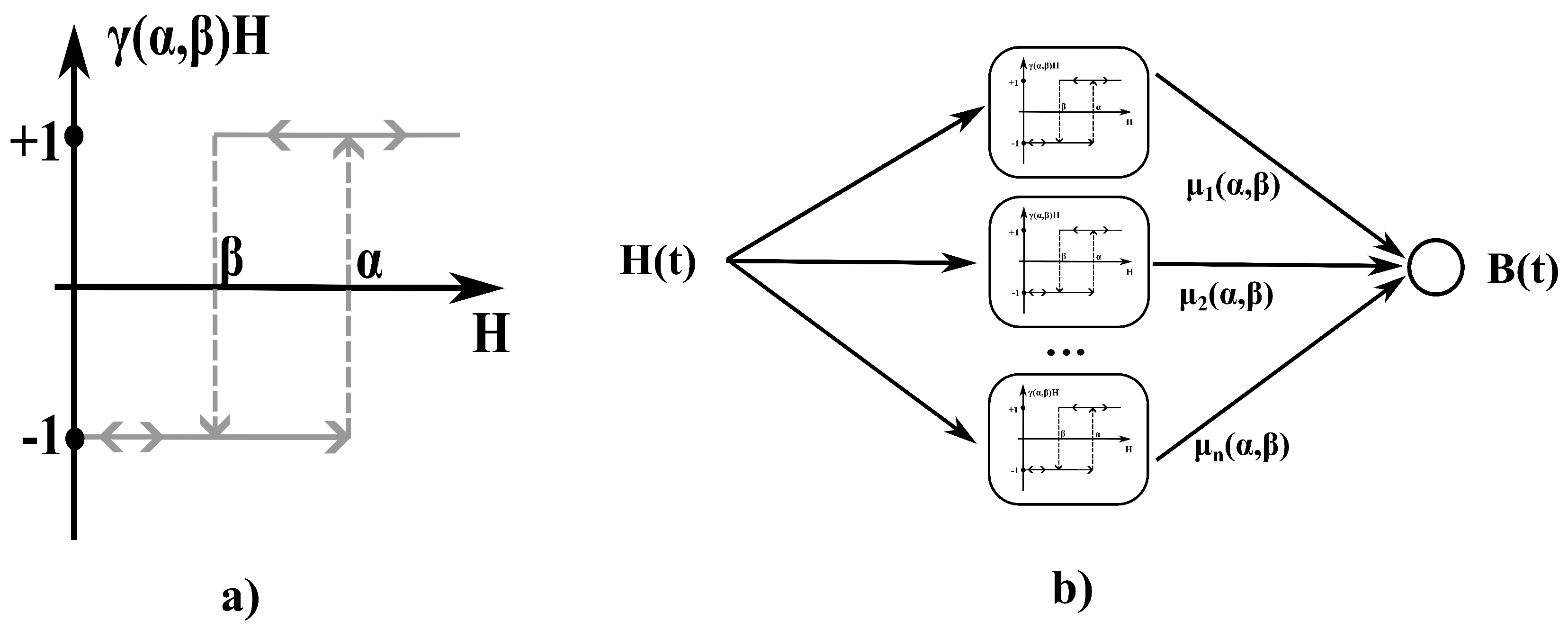
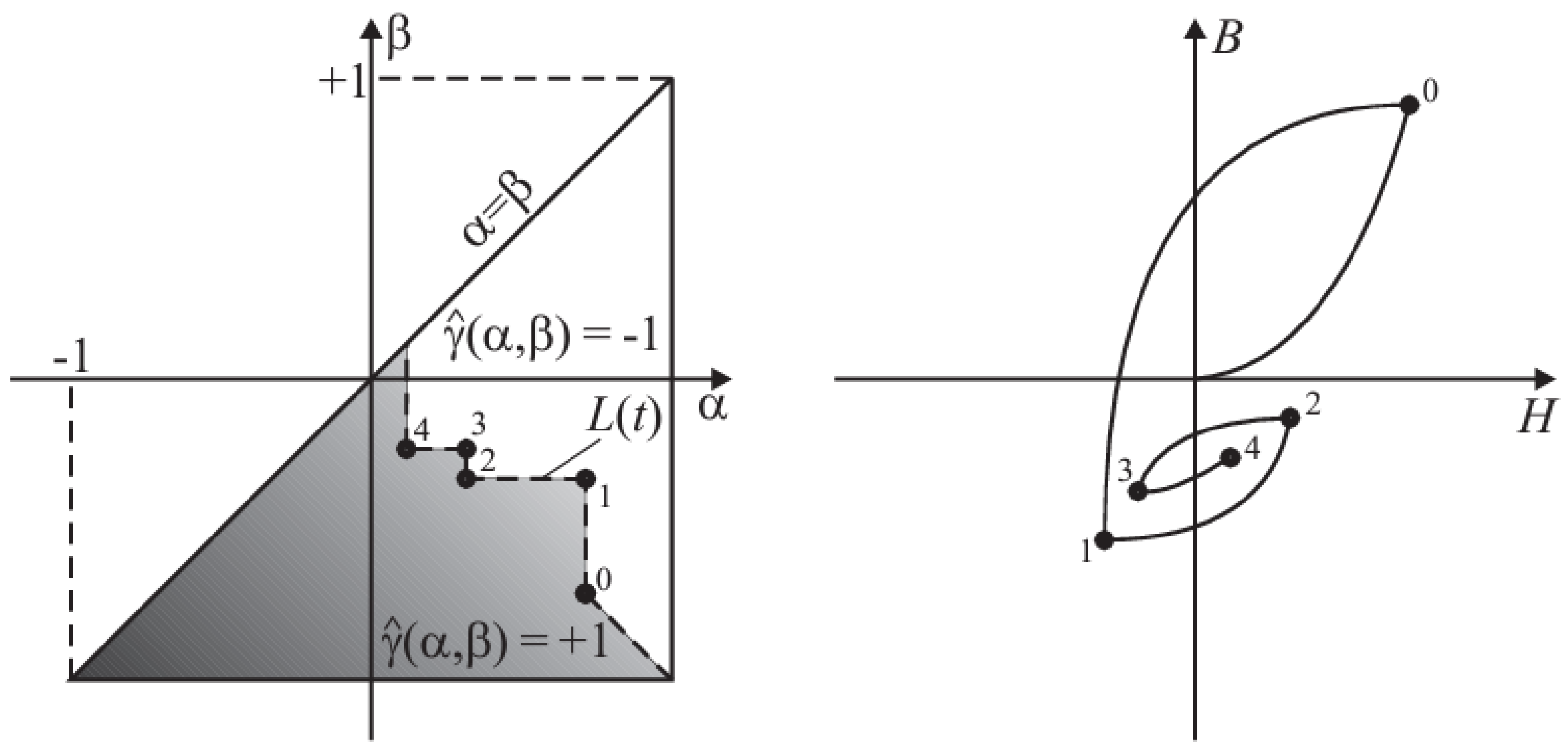
Classical Preisach-Model

One of the most-commonly used methods to approximate the hysteresis characteristic is the Preisach model [162,163,164,165]. According to this model, the resulting hysteresis characteristic is given by the weighted sum of the outputs of an infinite number of elementary hysteresis terms, defined by the following formula [162]:

$$B\left(t\right)=\mathcal{H}\left\{H\right\}={\int \int }_{\alpha \geqq \beta }\mu (\alpha ,\beta )\widehat{\gamma }(\alpha ,\beta )H\left(t\right)d\alpha d\beta .$$

(22)

The characteristics of hysteresis are shown in Figure 10 with an up value of $\alpha$, a down value of $\beta$, and $\alpha \geqq \beta$; its output takes only two values, so $\widehat{\gamma }(\alpha ,\beta )H=\pm 1$. $\mu (\alpha ,\beta )$ is the Preisach distribution function, which weights the output of each hysteresis. A block diagram representation of the Equation (22) is shown in Figure 10, where the parameters $\alpha$ and $\beta$ of each hysteresistakes different values in each parallel branch.

To describe this, the Preisach triangle was developed [30,162] and is shown in Figure 11. The Preisach triangle is the part of the plane $\alpha$−$\beta$ for which it is true that $\alpha \geqq \beta$. The prior life of the system is defined by the staircase line $L\left(t\right)$, which moves from left to right as the input signal increases and from top to bottom as the input signal decreases and couples the hysteresis terms $\alpha$ and $\beta$ with its movement. In the default position, the stepped curve connects the points (0; 0) and (+1; −1), thus bisecting the triangle. The corners of the staircase line are formed by the minimum and maximum values of the input signal, thus acting as a memory of the system.

Several approaches are published in the literature to resolve the double-integral in (22). Szabó decomposed the function in the dual-integral, which represents $\mu$, into a product of univariate Gaussian functions. In this way, the double-integral was reduced to a closed, analytic form [166,167]. Fuzi in [168] extended the Preisach distribution functions to approximate the main hysteresis loop better. Moreover, he introduced non-congruent minor behaviour. Because the original description of the Preisach model has two important mathematical properties, it has congruent minor loops and non-accommodating minor loops [151,160,169].

The Everett function [160,169] can be used efficiently instead of the distribution function, resulting in a model without the double-integral (22), i.e., the implemented model can be numerically more efficient than the previous approaches:

$$E(\alpha ,\beta )={\int \int }_{\alpha \geqq \beta }\mu (\xi ,\eta )\mathrm{d}\xi \mathrm{d}\eta .$$

(23)

The model output can then be obtained by

$$B\left(t\right)=-E({\alpha }_0,{\beta }_0)+2\sum _{k=1}^K[E({\alpha }_k,{\beta }_{k-1})-E({\alpha }_k,{\beta }_k)],$$

(24)

where K denotes the number of stairs in $L\left(t\right)$.

The other advantage of the Everett function is the direct connection with the measured first-order reversal curves or the concentric loops. The application of this methodology needs to resolve a computationally demanding parameter-determination process on the measurement results [170,171,172,173,174].

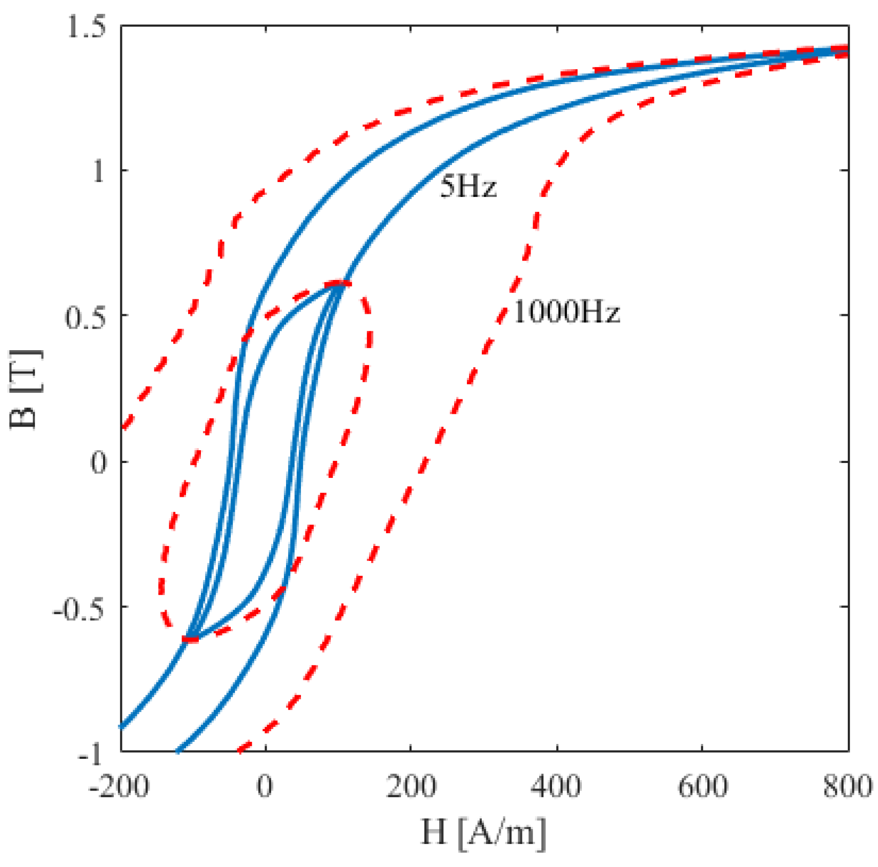
4.4. Dynamic Preisach Model

Due to the recent advances in electrical drives and electrical machine design, it was necessary to consider the frequency dependency of the losses more accurately during the machine design process [175,176].

The classical Preisach model does not consider frequency dependency. It only models the magnetic flux density as a function of the magnetic field intensity, i.e., $B=\mathcal{H}\left\{H\right\}$. Its inverse obtains the magnetic field intensity as a function of the magnetic flux density, i.e., $H=\mathcal{B}\left\{B\right\}$ [30,177,178]. Some authors refer to this dynamic Preisach model as the inverse Preisach model [164,179,180].

Magnetic field intensity is derived as the superposition of two terms: $H=H_{static}+H_{dynamic}$, where $H_{static}$ is given by the inverse static model and $H_{dynamic}$ is the magnetic field intensity due to dynamic effects. The approach in [175] builds up a surface $S(B,dB/dt)$, which is a function of two variables, the magnetic flux density and its variation. The Preisach distribution function can also be extended to consider the frequency dependency, i.e., applying $\mu (\alpha ,\beta ,f)$ [160,169]. These models are considered separately as loss surface models in the literature [30,175].

Hysteresis of a Lamination

The previous parts of this section showed how to model iron losses by simple formulas based on physical considerations. It is shown that standardised measurements can identify model parameters; afterwards, the models can approximate the losses via FEM-based simulations. The Steinmetz equation or the loss-separation-based formulas are used in the post-processing stage of finite-element simulations. Therefore, during the calculations, these methods cannot accurately consider the nonlinear B–H characteristics of every calculated finite-element. This section highlights how the complex Preisach model can be applied in FEM simulations to obtain the losses inside such a simple arrangement, i.e., inside a lamination made of material M250-35A. The simple illustration shows that applying the Preisach model results in accurate loss calculation; however, if the anomalous losses term extends it, it results in a time-consuming algorithm. In this case, obtaining a convergent algorithm can be difficult for a more-complex geometry. However, the calculated hysteresis loops at every finite-element cell of the arrangement can be more exact, which can benefit custom-designed electrical machines from SMLC materials. Two kinds of Preisach-type models are applied in this section for a simple lamination to estimate the losses of the selected M250-35A-grade steel and demonstrate the applicability of the Preisach models.

The quasi-static Maxwell’s equations can approximate electromagnetic fields inside a lamination [162,181]:

$$\begin{array}{cc}\hfill \nabla \times \mathit{H}& =\sigma \mathit{E},\hfill \\ \hfill \nabla \times \mathit{E}& =-\frac{\partial \mathit{B}}{\partial t},\hfill \\ \hfill \nabla ·\mathit{B}& =0,\hfill \end{array}$$

(25)

where $\mathit{H}$ is the magnetic field intensity, $\mathit{E}$ is the electric field intensity, $\sigma \mathit{E}$ is the eddy current with the conductivity denoted by $\sigma$, and $\mathit{B}$ is the magnetic flux density.

A one-dimensional finite-element-method-based code was implemented in Matlab to approximate the electromagnetic fields and the losses inside the lamination. Maxwell’s equations have the following simpler formula in 1D:

$$\begin{array}{cc}\hfill \frac{\partial H_y}{\partial x}& =\sigma E_z,\hfill \\ \hfill \frac{\partial E_z}{\partial x}& =\frac{\partial B_y}{\partial t}.\hfill \end{array}$$

(26)

The equation $\nabla ·\mathit{B}=0$ is satisfied automatically. It is supposed that the magnetic field intensity and the magnetic flux density have only components in the y axis ($H_y$ and $B_y$), and the electric field intensity only varies along the z axis ($E_z$). The lamination depth is in the x axis [162,181].

The constitutive relationship between the magnetic field intensity and the magnetic flux density is given by the polarisation formulation [162,182], i.e.,

$$B_y=\mu (H_y-H_{y,\mathrm{exc}})+R_y.$$

(27)

The term $H_y-H_{y,\mathrm{exc}}$ is the input magnetic field intensity of the Preisach model and $\mu$ is constant:

$$\mu =\frac{{\mu }_{max}+{\mu }_{min}}{2},$$

(28)

where ${\mu }_{max}$ and ${\mu }_{min}$ are the characteristics’ maximum and minimum slope [182]. The excess field term can be expressed according to the viscous-type model as follows [183]:

$$H_{y,\mathrm{exc}}=\delta {\left|\frac{1}{r\left(B_y\right)}\frac{\mathrm{d}{B}_y}{\mathrm{d}t}\right|}^{1/\gamma },\mathrm{and}r\left(B_y\right)=\frac{R_0}{1-{\left(\frac{B_y}{B_s}\right)}^2},$$

(29)

where $\delta$ is positive or negative along an increasing or decreasing curve of the hysteresis loop, respectively, and $\gamma$ and $r\left(B_y\right)$ measure the dynamic loops. The fixed-point iteration scheme gives the residual term $R_y$. The lamination is made of the ferromagnetic material M250-35A with $R_0=23.79$ and $\gamma =1$.

After a short manipulation, the following partial differential equation can be obtained:

$$-\frac{{\partial }^2{H}_y}{\partial x^2}+\mu \sigma \frac{\partial H_y}{\partial t}=\mu \sigma \frac{\partial H_{y,\mathrm{exc}}}{\partial t}-\sigma \frac{\partial R_y}{\partial t}.$$

(30)

This nonlinear partial differential equation is solved by the finite-element method at every time instant of the source magnetic field defined as a sinusoid. The fixed-point algorithm of a time step to solve the nonlinear problem is as follows [162,182]:

• Solve (30) by the finite-element method (start with the value of $R_y$ and $H_{y,exc}$ of the previous time instant), which gives $H_y$ at every node of the mesh;
• The magnetic flux density $B_y$ at every node can be obtained by the Preisach model with the input of $H_y-H_{y,exc}$;
• The residual term $R_y$ is given by rearranging (27), i.e., $R_y=B_y-\mu (H_y-H_{y,\mathrm{exc}})$;
• The term $H_{y,exc}$ is updated by (29).

These steps are repeated until convergence.

The total loss P can be obtained by

$$P=\frac{1}{T\rho }{\int }_0^T{H}_y\frac{\mathrm{d}{B}_y}{\mathrm{d}t}\mathrm{d}t,$$

(31)

where $H_y$ and $B_y$ are the magnetic field intensity at the finite-element node of the lamination surface and the magnetic flux density averaged over the lamination, the mass density of the lamination material is denoted by $\rho$, $\rho =7600\mathrm{kg}/{\mathrm{m}}^3$, and T represents the examined time period. The unit of P is Watts per kilogram.

Table 1. Comparison of simulated (eddy current only/extended) and measured losses.

B [T]	P @ 5 Hz	P @ 50 Hz	P @ 100 Hz	P @ 200 Hz
0.2	0.01/0.01 (0.01)	0.08/0.093 (0.08)	0.17/0.22 (0.21)	0.39/0.55 (0.55)
0.6	0.05/0.05 (0.05)	0.54/0.616 (0.60)	1.16/1.49 (1.52)	2.67/3.98 (4.10)
1.0	0.12/0.12 (0.12)	1.30/1.50 (1.38)	2.85/3.66 (3.74)	6.69/9.96 (9.96)
1.4	0.23/0.23 (0.22)	2.53/2.85 (2.57)	5.54/6.87 (6.78)	13.1/18.4 (17.7)

presents a comparison between the simulated iron losses and the iron loss data obtained from the measured curves performed by our hysteresis loop measurement system [117]. The measured data are given in parentheses. The above-mentioned finite-element-method-based eddy current field simulation gives simulated iron loss data. The measured hysteresis loops were used to identify the classical and the extended Preisach model. Two simulated loss data are given in Table 1, calculated without and with the excess loss term $H_{y,\mathrm{exc}}$. The results obtained by the static Preisach model (when $H_{y,\mathrm{exc}}=0$) take only eddy currents into account, and excess losses are neglected, while excess losses can be taken into account by applying the term $H_{y,\mathrm{exc}}$.

Some simulated hysteresis loops are depicted in Figure 12, where the effect of eddy currents, as well as excess losses can be seen, i.e., the hysteresis loop is increased by the increased frequency. Some comparisons between the measured and simulated data can be studied in Figure 13, where concentric minor loops and higher-order minor loops are generated and simulated.

Calculating with a function implementing the Preisach model accounts for about 80–90% of the total finite-element-method-based calculation. The generation of the required values of the Everett function within the Preisach model is about 95–97% of the total model run.

5. Conclusions

Three-dimensional printing is a promising technology for creating iron cores for electrical machines. However, the applied materials are still expensive. It can be an economical technology for creating rapid prototypes of iron cores or custom-manufactured machines with complex geometries. One possible material is the Fe-6.5wt%Si silicon steel alloy, which can reduce the operating and operation costs. However, it is incredibly brittle due to its high silicon content. An exciting possibility with this technology is that the formation of the magnetic domain structure can be directed by applying an appropriate magnetic field during the printing process. FeSi alloys are promising materials for creating competitive electrical machine designs in the future. However, improving the ductility of this material is not enough to harness the full potential of this material. A better understanding of the magnetisation process and a deep knowledge of the numerical iron loss calculation methods are necessary to create more-competitive electrical machine designs. The second part of the paper overviewed the applicable measurement methodologies and iron loss calculation methods. Most of the proposed methodologies can be used to calculate the losses in 3D-printed materials. However, the Preisach- or Play-model-based calculations seem to be the most-promising iron loss models. Besides their high accuracy, the application of these models requires an extensive measurement methodology; the direct application of this methodology on 3D-printed prototypes is not straightforward, but a challenging problem.

References

1. Kang, N.; El Mansori, M.; Guittonneau, F.; Liao, H.; Fu, Y.; Aubry, E. Controllable mesostructure, magnetic properties of soft magnetic Fe-Ni-Si by using selective laser melting from nickel coated high silicon steel powder. Appl. Surf. Sci. 2018, 455, 736–741. [Google Scholar] [CrossRef]
2. Lemke, J.; Simonelli, M.; Garibaldi, M.; Ashcroft, I.; Hague, R.; Vedani, M.; Wildman, R.; Tuck, C. Calorimetric study and microstructure analysis of the order-disorder phase transformation in silicon steel built by SLM. J. Alloys Compd. 2017, 722, 293–301. [Google Scholar] [CrossRef]
3. Garibaldi, M.; Ashcroft, I.; Lemke, J.; Simonelli, M.; Hague, R. Effect of annealing on the microstructure and magnetic properties of soft magnetic Fe-Si produced via laser additive manufacturing. Scr. Mater. 2018, 142, 121–125. [Google Scholar] [CrossRef]
4. Garibaldi, M.; Ashcroft, I.; Hillier, N.; Harmon, S.; Hague, R. Relationship between laser energy input, microstructures and magnetic properties of selective laser melted Fe-6.9. Mater. Charact. 2018, 143, 144–151. [Google Scholar] [CrossRef]
5. Żrodowski, Ł.; Wysocki, B.; Wrblewski, R.; Krawczyska, A.; Adamczyk-Cielak, B.; Zdunek, J.; Byskun, P.; Ferenc, J.; Leonowicz, M.; wiszkowski, W. New approach to amorphization of alloys with low glass forming ability via selective laser melting. J. Alloys Compd. 2019, 771, 769–776. [Google Scholar] [CrossRef]
6. Goll, D.; Schuller, D.; Martinek, G.; Kunert, T.; Schurr, J.; Sinz, C.; Schubert, T.; Bernthaler, T.; Riegel, H.; Schneider, G. Additive manufacturing of soft magnetic materials and components. Addit. Manuf. 2019, 27, 428–439. [Google Scholar] [CrossRef]
7. Heer, B.; Bandyopadhyay, A. Compositionally graded magnetic-nonmagnetic bimetallic structure using laser engineered net shaping. Mater. Lett. 2018, 216, 16–19. [Google Scholar] [CrossRef]
8. Ayat, S.; Simpson, N.; Dagus, B.; Rudolph, J.; Lorenz, F.; Drury, D. Design of Shaped-Profile Electrical Machine Windings for Multi-Material Additive Manufacture. In Proceedings of the 2020 International Conference on Electrical Machines (ICEM), Gothenburg, Sweden, 23–26 August 2020; Volume 1, pp. 1554–1559. [Google Scholar] [CrossRef]
9. Garibaldi, M. Laser Additive Manufacturing of Soft Magnetic Cores for Rotating Electrical Machinery: Materials Development and Part Design. Ph.D. Thesis, University of Nottingham, Nottingham, UK, 2018. [Google Scholar]
10. Sarap, M.; Kallaste, A.; Shams Ghahfarokhi, P.; Tiismus, H.; Vaimann, T. Utilization of additive manufacturing in the thermal design of electrical machines: A review. Machines 2022, 10, 251. [Google Scholar] [CrossRef]
11. Giannotta, N.; Sala, G.; Bianchini, C.; Torreggiani, A. A Review of Additive Manufacturing of Soft Magnetic Materials in Electrical Machines. Machines 2023, 11, 702. [Google Scholar] [CrossRef]
12. Ghahfarokhi, P.S.; Podgornovs, A.; Kallaste, A.; Cardoso, A.J.M.; Belahcen, A.; Vaimann, T.; Tiismus, H.; Asad, B. Opportunities and Challenges of Utilizing Additive Manufacturing Approaches in Thermal Management of Electrical Machines. IEEE Access 2021, 9, 36368–36381. [Google Scholar] [CrossRef]
13. Hernandez, M.; Messagie, M.; Hegazy, O.; Marengo, L.; Winter, O.; Van Mierlo, J. Environmental impact of traction electric motors for electric vehicles applications. Int. J. Life Cycle Assess. 2017, 22, 54–65. [Google Scholar] [CrossRef]
14. Horváth, C. The Current Situation of the Rare-Earth Material Usage in the Field of Electromobility. In Proceedings of the Vehicle and Automotive Engineering 4; Jármai, K., Cservenák, Á., Eds.; Springer International Publishing: Cham, Switzerland, 2023; pp. 493–504. [Google Scholar] [CrossRef]
15. Schoppa, A.; Delarbre, P.; Holzmann, E.; Sigl, M. Magnetic properties of soft magnetic powder composites at higher frequencies in comparison with electrical steels. In Proceedings of the 2013 3rd International Electric Drives Production Conference (EDPC), Nuremberg, Germany, 29–30 October 2013; pp. 1–5. [Google Scholar] [CrossRef]
16. Landgraf, F.; Emura, M.; Teixeira, J.; de Campos, M. Effect of grain size, deformation, aging and anisotropy on hysteresis loss of electrical steels. J. Magn. Magn. Mater. 2000, 215–216, 97–99. [Google Scholar] [CrossRef]
17. Naumoski, H.; Riedmller, B.; Minkow, A.; Herr, U. Investigation of the influence of different cutting procedures on the global and local magnetic properties of non-oriented electrical steel. J. Magn. Magn. Mater. 2015, 392, 126–133. [Google Scholar] [CrossRef]
18. Kalsoom, U.; Nesterenko, P.N.; Paull, B. Recent developments in 3D printable composite materials. RSC Adv. 2016, 6, 60355–60371. [Google Scholar] [CrossRef]
19. Pham, T.; Kwon, P.; Foster, S. Additive manufacturing and topology optimization of magnetic materials for electrical machines—A review. Energies 2021, 14, 283. [Google Scholar] [CrossRef]
20. Andreiev, A.; Hoyer, K.P.; Hengsbach, F.; Haase, M.; Tasche, L.; Duschik, K.; Schaper, M. Powder bed fusion of soft-magnetic iron-based alloys with high silicon content. J. Mater. Process. Technol. 2023, 317, 117991. [Google Scholar] [CrossRef]
21. Andreiev, A.; Hoyer, K.P.; Dula, D.; Hengsbach, F.; Haase, M.; Gierse, J.; Zimmer, D.; Tröster, T.; Schaper, M. Soft-magnetic behavior of laser beam melted FeSi3 alloy with graded cross-section. J. Mater. Process. Technol. 2021, 296, 117183. [Google Scholar] [CrossRef]
22. Garibaldi, M.; Ashcroft, I.; Simonelli, M.; Hague, R. Metallurgy of high-silicon steel parts produced using Selective Laser Melting. Acta Mater. 2016, 110, 207–216. [Google Scholar] [CrossRef]
23. Wu, W.; Li, X.; Liu, Q.; Fuh, J.Y.H.; Zheng, A.; Zhou, Y.; Ren, L.; Li, G. Additive manufacturing of bulk metallic glass: Principles, materials and prospects. Mater. Today Adv. 2022, 16, 100319. [Google Scholar] [CrossRef]
24. Kocsis, B.; Hatos, I.; Varga, L.K. 3D-printed metal–insulator layered structure. J. Magn. Magn. Mater. 2022, 563, 169994. [Google Scholar] [CrossRef]
25. Nam, Y.G.; Koo, B.; Chang, M.S.; Yang, S.; Yu, J.; Park, Y.H.; Jeong, J.W. Selective laser melting vitrification of amorphous soft magnetic alloys with help of double-scanning-induced compositional homogeneity. Mater. Lett. 2020, 261, 127068. [Google Scholar] [CrossRef]
26. Bence, K. Fém-Szigetelő Kompozitok Előállítása Járműipari célú Felhasználáshoz. Ph.D. Thesis, Széchenyi István University, Győr, Hungary, 2023. [Google Scholar]
27. M270 Steel BH Curve Data. Available online: https://doc.modelica.org/Modelica%203.2.3/Resources/helpMapleSim/Magnetic/FluxTubes/Material/HysteresisTableData/index.html (accessed on 10 August 2023).
28. Bali, M. Magnetic Material Degradation Due to Different Cutting Techniques and Its Modeling for Electric Machine Design. Ph.D. Thesis, Technischen Universitat Graz, Graz, Austria, 2016. [Google Scholar]
29. Tiismus, H.; Kallaste, A.; Belahcen, A.; Tarraste, M.; Vaimann, T.; Rasslkin, A.; Asad, B.; Shams Ghahfarokhi, P. AC Magnetic Loss Reduction of SLM Processed Fe-Si for Additive Manufacturing of Electrical Machines. Energies 2021, 14, 1241. [Google Scholar] [CrossRef]
30. Krings, A. Iron Losses in Electrical Machines-Influence of Material Properties, Manufacturing Processes, and Inverter Operation. Ph.D. Thesis, KTH Royal Institute of Technology, Stockholm, Sweden, 2014. [Google Scholar]
31. Lee, J.; Seo, J.H.; Kikuchi, N. Topology optimization of switched reluctance motors for the desired torque profile. Struct. Multidiscip. Optim. 2010, 42, 783–796. [Google Scholar] [CrossRef]
32. Kim, D.H.; Sykulski, J.K.; Lowther, D.A. The implications of the use of composite materials in electromagnetic device topology and shape optimization. IEEE Trans. Magn. 2009, 45, 1154–1157. [Google Scholar] [CrossRef]
33. Tiismus, H.; Kallaste, A.; Vaimann, T.; Rassõlkin, A. State of the art of additively manufactured electromagnetic materials for topology optimized electrical machines. Addit. Manuf. 2022, 55, 102778. [Google Scholar] [CrossRef]
34. Koopmann, J.; Voigt, J.; Niendorf, T. Additive manufacturing of a steel–ceramic multi-material by selective laser melting. Metall. Mater. Trans. B 2019, 50, 1042–1051. [Google Scholar] [CrossRef]
35. Kocsis, B.; Fekete, I.; Varga, L. Metallographic and magnetic analysis of direct laser sintered soft magnetic composites. J. Magn. Magn. Mater. 2020, 501, 166425. [Google Scholar] [CrossRef]
36. Ding, C.; Liu, L.; Mei, Y.; Ngo, K.D.; Lu, G.Q. Magnetic paste as feedstock for additive manufacturing of power magnetics. In Proceedings of the 2018 IEEE Applied Power Electronics Conference and Exposition (APEC), San Antonio, TX, USA, 4–8 March 2018; pp. 615–618. [Google Scholar]
37. Lin, P.H.; Yang, B.Y.; Tsai, M.H.; Chen, P.C.; Huang, K.F.; Lin, H.H.; Lai, C.H. Manipulating exchange bias by spin–orbit torque. Nat. Mater. 2019, 18, 335–341. [Google Scholar] [CrossRef]
38. Cramer, C.L.; Nandwana, P.; Yan, J.; Evans, S.F.; Elliott, A.M.; Chinnasamy, C.; Paranthaman, M.P. Binder jet additive manufacturing method to fabricate near net shape crack-free highly dense Fe-6.5 wt.% Si soft magnets. Heliyon 2019, 5, e02804. [Google Scholar] [CrossRef]
39. Kustas, A.B.; Susan, D.F.; Johnson, K.L.; Whetten, S.R.; Rodriguez, M.A.; Dagel, D.J.; Michael, J.R.; Keicher, D.M.; Argibay, N. Characterization of the Fe-Co-1.5 V soft ferromagnetic alloy processed by Laser Engineered Net Shaping (LENS). Addit. Manuf. 2018, 21, 41–52. [Google Scholar]
40. Khatri, B.; Lappe, K.; Noetzel, D.; Pursche, K.; Hanemann, T. A 3D-Printable Polymer-Metal Soft-Magnetic Functional Composite—Development and Characterization. Materials 2018, 11, 189. [Google Scholar] [CrossRef] [PubMed]
41. Liu, L.; Ge, T.; Ngo, K.D.T.; Mei, Y.; Lu, G.Q. Ferrite Paste Cured With Ultraviolet Light for Additive Manufacturing of Magnetic Components for Power Electronics. IEEE Magn. Lett. 2018, 9, 1–5. [Google Scholar] [CrossRef]
42. Kokkinis, D.; Schaffner, M.; Studart, A.R. Multimaterial magnetically assisted 3D printing of composite materials. Nat. Commun. 2015, 6, 8643. [Google Scholar] [CrossRef] [PubMed]
43. Paranthaman, M.P.; Shafer, C.S.; Elliott, A.M.; Siddel, D.H.; McGuire, M.A.; Springfield, R.M.; Martin, J.; Fredette, R.; Ormerod, J. Binder Jetting: A Novel NdFeB Bonded Magnet Fabrication Process. Jom 2016, 68, 1978–1982. [Google Scholar] [CrossRef]
44. Shahrubudin, N.; Lee, T.C.; Ramlan, R. An overview on 3D printing technology: Technological, materials, and applications. Procedia Manuf. 2019, 35, 1286–1296. [Google Scholar] [CrossRef]
45. Szabó, L.; Fodor, D. The key role of 3D printing technologies in the further development of electrical machines. Machines 2022, 10, 330. [Google Scholar] [CrossRef]
46. Kallaste, A.; Vaimann, T.; Rassãlkin, A. Additive design possibilities of electrical machines. In Proceedings of the 2018 IEEE 59th International Scientific Conference on Power and Electrical Engineering of Riga Technical University (RTUCON), Riga, Latvia, 12–13 November 2018; pp. 1–5. [Google Scholar]
47. Snoek, J. Dispersion and absorption in magnetic ferrites at frequencies above one Mc/s. Physica 1948, 14, 207–217. [Google Scholar] [CrossRef]
48. Mager, A. About the influence of grain size on the coercivity. Ann. Phys. Leipzig 1952, 446, 15–16. [Google Scholar] [CrossRef]
49. Hu, Y.; Cong, W. A review on laser deposition-additive manufacturing of ceramics and ceramic reinforced metal matrix composites 2018. Ceram. Int. 2018, 44, 20599–20612. [Google Scholar] [CrossRef]
50. Zhang, H.; LeBlanc, S. Processing parameters for selective laser sintering or melting of oxide ceramics. Addit. Manuf.-High-Perform. Met.-Alloy.-Model. Optim. 2018, 10, 1–44. [Google Scholar]
51. Nakai, Y.; Mishima, F.; Akiyama, Y.; Nishijima, S. Development of magnetic separation system for powder separation. IEEE Trans. Appl. Supercond. 2010, 20, 941–944. [Google Scholar] [CrossRef]
52. Gibson, I.; Rosen, D.; Stucker, B.; Khorasani, M.; Gibson, I.; Rosen, D.; Stucker, B.; Khorasani, M. Materials for additive manufacturing. Addit. Manuf. Technol. 2021, 379–428. [Google Scholar]
53. Sahasrabudhe, H.; Bandyopadhyay, A. Additive Manufacturing of Reactive In Situ Zr Based Ultra-High Temperature Ceramic Composites. Jom 2016, 68, 822–830. [Google Scholar] [CrossRef]
54. Fan, Z.; Zhao, Y.; Tan, Q.; Mo, N.; Zhang, M.X.; Lu, M.; Huang, H. Nanostructured Al2O3-YAG-ZrO2 ternary eutectic components prepared by laser engineered net shaping. Acta Mater. 2019, 170, 24–37. [Google Scholar] [CrossRef]
55. Zheng, B.; Topping, T.; Smugeresky, J.E.; Zhou, Y.; Biswas, A.; Baker, D.; Lavernia, E.J. The Influence of Ni-Coated TiC on Laser-Deposited IN625 Metal Matrix Composites. Metall. Mater. Trans. A 2010, 41, 568–573. [Google Scholar] [CrossRef]
56. Shen, M.Y.; Tian, X.J.; Liu, D.; Tang, H.B.; Cheng, X. Microstructure and fracture behavior of TiC particles reinforced Inconel 625 composites prepared by laser additive manufacturing. J. Alloys Compd. 2018, 734, 188–195. [Google Scholar] [CrossRef]
57. Tan, H.; Hao, D.; Al-Hamdani, K.; Zhang, F.; Xu, Z.; Clare, A.T. Direct metal deposition of TiB2/AlSi10Mg composites using satellited powders. Mater. Lett. 2018, 214, 123–126. [Google Scholar] [CrossRef]
58. Cao, S.; Gu, D.; Shi, Q. Relation of microstructure, microhardness and underlying thermodynamics in molten pools of laser melting deposition processed TiC/Inconel 625 composites. J. Alloys Compd. 2017, 692, 758–769. [Google Scholar] [CrossRef]
59. Farayibi, P.; Abioye, T.; Kennedy, A.; Clare, A. Development of metal matrix composites by direct energy deposition of satellited powders. J. Manuf. Process. 2019, 45, 429–437. [Google Scholar] [CrossRef]
60. Huang, Y.; Wu, D.; Zhao, D.; Niu, F.; Zhang, H.; Yan, S.; Ma, G. Process optimization of melt growth alumina/aluminum titanate composites directed energy deposition: Effects of scanning speed. Addit. Manuf. 2020, 35, 101210. [Google Scholar] [CrossRef]
61. Amar, A.; Li, J.; Xiang, S.; Liu, X.; Zhou, Y.; Le, G.; Wang, X.; Qu, F.; Ma, S.; Dong, W.; et al. Additive manufacturing of high-strength CrMnFeCoNi-based High Entropy Alloys with TiC addition. Intermetallics 2019, 109, 162–166. [Google Scholar] [CrossRef]
62. Svetlizky, D.; Zheng, B.; Vyatskikh, A.; Das, M.; Bose, S.; Bandyopadhyay, A.; Schoenung, J.M.; Lavernia, E.J.; Eliaz, N. Laser-based directed energy deposition (DED-LB) of advanced materials. Mater. Sci. Eng. A 2022, 840, 142967. [Google Scholar] [CrossRef]
63. Traxel, K.D.; Bandyopadhyay, A. Naturally architected microstructures in structural materials via additive manufacturing. Addit. Manuf. 2020, 34, 101243. [Google Scholar] [CrossRef]
64. Zou, J.; Gaber, Y.; Voulazeris, G.; Li, S.; Vazquez, L.; Liu, L.F.; Yao, M.Y.; Wang, Y.J.; Holynski, M.; Bongs, K.; et al. Controlling the grain orientation during laser powder bed fusion to tailor the magnetic characteristics in a Ni-Fe based soft magnet. Acta Mater. 2018, 158, 230–238. [Google Scholar] [CrossRef]
65. De Oliveira, A.R.; De Oliveira, V.F.; Teixeira, J.C.; Del Conte, E.G. Investigation of the build orientation effect on magnetic properties and Barkhausen Noise of additively manufactured maraging steel 300. Addit. Manuf. 2021, 38, 101827. [Google Scholar] [CrossRef]
66. Ouyang, D.; Li, N.; Xing, W.; Zhang, J.; Liu, L. 3D printing of crack-free high strength Zr-based bulk metallic glass composite by selective laser melting. Intermetallics 2017, 90, 128–134. [Google Scholar] [CrossRef]
67. Jung, H.Y.; Choi, S.J.; Prashanth, K.G.; Stoica, M.; Scudino, S.; Yi, S.; Kühn, U.; Kim, D.H.; Kim, K.B.; Eckert, J. Fabrication of Fe-based bulk metallic glass by selective laser melting: A parameter study. Mater. Des. 2015, 86, 703–708. [Google Scholar] [CrossRef]
68. Shen, Y.; Li, Y.; Chen, C.; Tsai, H.L. 3D printing of large, complex metallic glass structures. Mater. Des. 2017, 117, 213–222. [Google Scholar] [CrossRef]
69. Borkar, T.; Conteri, R.; Chen, X.; Ramanujan, R.; Banerjee, R. Laser additive processing of functionally-graded Fe–Si–B–Cu–Nb soft magnetic materials. Mater. Manuf. Process. 2017, 32, 1581–1587. [Google Scholar] [CrossRef]
70. Gibson, M.A.; Mykulowycz, N.M.; Shim, J.; Fontana, R.; Schmitt, P.; Roberts, A.; Ketkaew, J.; Shao, L.; Chen, W.; Bordeenithikasem, P.; et al. 3D printing metals like thermoplastics: Fused filament fabrication of metallic glasses. Mater. Today 2018, 21, 697–702. [Google Scholar] [CrossRef]
71. Arnold, H.; Elmen, G. Bell System Tech. J. USA Tel. Tel. 1923, 2, 101. [Google Scholar]
72. Redjdal, N.; Salah, H.; Hauet, T.; Menari, H.; Chérif, S.; Gabouze, N.; Azzaz, M. Microstructural, electrical and magnetic properties of Fe35Co65 thin films grown by thermal evaporation from mechanically alloyed powders. Thin Solid Films 2014, 552, 164–169. [Google Scholar] [CrossRef]
73. Schönrath, H.; Spasova, M.; Kilian, S.; Meckenstock, R.; Witt, G.; Sehrt, J.; Farle, M. Additive manufacturing of soft magnetic permalloy from Fe and Ni powders: Control of magnetic anisotropy. J. Magn. Magn. Mater. 2019, 478, 274–278. [Google Scholar] [CrossRef]
74. Ouyang, G.; Chen, X.; Liang, Y.; Macziewski, C.; Cui, J. Review of Fe-6.5 wt% Si high silicon steelA promising soft magnetic material for sub-kHz application. J. Magn. Magn. Mater.s 2019, 481, 234–250. [Google Scholar] [CrossRef]
75. Plotkowski, A.; Carver, K.; List, F.; Pries, J.; Li, Z.; Rossy, A.M.; Leonard, D. Design and performance of an additively manufactured high-Si transformer core. Mater. Des. 2020, 194, 108894. [Google Scholar] [CrossRef]
76. Goodall, A.D.; Chechik, L.; Mitchell, R.L.; Jewell, G.W.; Todd, I. Cracking of soft magnetic FeSi to reduce eddy current losses in stator cores. Addit. Manuf. 2023, 70, 103555. [Google Scholar] [CrossRef]
77. Magnetic Materials Part 2: Methods of Measurement of the Magnetic Properties of Electrical Steel Strip and Sheet by Means of an Epstein Frame; Standard, International Electrotechnical Commission: London, UK, 2008.
78. Magnetic Materials Part 4: Methods of Measurement of the Magnetic Properties of Magnetic Sheet and Strip by Means of a Single Sheet Tester; Standard, International Electrotechnical Commission: London, UK, 2010.
79. Magnetic Materials Part 6: Methods of Measurement of the Magnetic Properties of Magnetically Soft Metallic and Powder Materials at Frequencies in the Range 20 Hz to 100 kHz by the Use of Ring Specimens; Standard, International Electrotechnical Commission: London, UK, 2018.
80. Fiorillo, F. Measurements of magnetic materials. Metrologia 2010, 47, S114. [Google Scholar] [CrossRef]
81. Selema, A.; Beretta, M.; Van Coppenolle, M.; Tiismus, H.; Kallaste, A.; Ibrahim, M.N.; Rombouts, M.; Vleugels, J.; Kestens, L.A.; Sergeant, P. Evaluation of 3D-Printed Magnetic Materials For Additively-Manufactured Electrical Machines. J. Magn. Magn. Mater. 2023, 569, 170426. [Google Scholar] [CrossRef]
82. Tiismus, H.; Kallaste, A.; Belahcen, A.; Vaimann, T.; Rassõlkin, A.; Lukichev, D. Hysteresis measurements and numerical losses segregation of additively manufactured silicon steel for 3D printing electrical machines. Appl. Sci. 2020, 10, 6515. [Google Scholar] [CrossRef]
83. Bramerdorfer, G.; Kitzberger, M.; Wckinger, D.; Koprivica, B.; Zurek, S. State-of-the-art and future trends in soft magnetic materials characterization with focus on electric machine design Part 1. TM-Tech. Mess. 2019, 86, 540–552. [Google Scholar] [CrossRef]
84. Antonelli, E.; Cardelli, E.; Faba, A. Epstein frame: How and when it can be really representative about the magnetic behavior of laminated magnetic steels. IEEE Trans. Magn. 2005, 41, 1516–1519. [Google Scholar] [CrossRef]
85. Pham, T.Q.; Mellak, C.; Suen, H.; Boehlert, C.J.; Muetze, A.; Kwon, P.; Foster, S.N. Binder Jet Printed Iron Silicon with Low Hysteresis Loss. In Proceedings of the 2019 IEEE International Electric Machines & Drives Conference (IEMDC), San Diego, CA, USA, 12–15 May 2019; pp. 1045–1052. [Google Scholar] [CrossRef]
86. Yamamoto, T.; Ohya, Y. Single sheet tester for measuring core losses and permeabilities in a silicon steel sheet. IEEE Trans. Magn. 1974, 10, 157–159. [Google Scholar] [CrossRef]
87. Li, Y.; Zhu, J.; Yang, Q.; Lin, Z.W.; Guo, Y.; Zhang, C. Study on rotational hysteresis and core loss under three-dimensional magnetization. IEEE Trans. Magn. 2011, 47, 3520–3523. [Google Scholar] [CrossRef]
88. Plotkowski, A.; Pries, J.; List, F.; Nandwana, P.; Stump, B.; Carver, K.; Dehoff, R. Influence of scan pattern and geometry on the microstructure and soft-magnetic performance of additively manufactured Fe-Si. Addit. Manuf. 2019, 29, 100781. [Google Scholar] [CrossRef]
89. Serrano, D.; Li, H.; Wang, S.; Guillod, T.; Luo, M.; Bansal, V.; Jha, N.K.; Chen, Y.; Sullivan, C.R.; Chen, M. Why MagNet: Quantifying the Complexity of Modeling Power Magnetic Material Characteristics. IEEE Trans. Power Electron. 2023, 1–25. [Google Scholar] [CrossRef]
90. Smith, A.; Edey, K. Influence of manufacturing processes on iron losses. In Proceedings of the Seventh International Conference on Electrical Machines and Drives, Durham, UK, 11–13 September 1995. [Google Scholar]
91. Bramerdorfer, G.; Kitzberger, M.; Wöckinger, D.; Koprivica, B.; Zurek, S. State-of-the-art and future trends in soft magnetic materials characterization with focus on electric machine design–Part 2. TM-Tech. Mess. 2019, 86, 553–565. [Google Scholar] [CrossRef]
92. Michaelides, A.; Simkin, J.; Kirby, P.; Riley, C. Permanent magnet (de-) magnetization and soft iron hysteresis effects: A comparison of FE analysis techniques. COMPEL- Int. J. Comput. Math. Electr. Electron. Eng. 2010, 29, 1090–1096. [Google Scholar] [CrossRef]
93. Zirka, S.; Moroz, Y.I. Hysteresis modeling based on transplantation. IEEE Trans. Magn. 1995, 31, 3509–3511. [Google Scholar] [CrossRef]
94. Steinmetz, C.P. On the law of hysteresis. Trans. Am. Inst. Electr. Eng. 1892, 9, 1–64. [Google Scholar] [CrossRef]
95. Venkatachalam, K.; Sullivan, C.R.; Abdallah, T.; Tacca, H. Accurate prediction of ferrite core loss with nonsinusoidal waveforms using only Steinmetz parameters. In Proceedings of the 2002 IEEE Workshop on Computers in Power Electronics, Mayaguez, PR, USA, 3–4 June 2002; pp. 36–41. [Google Scholar]
96. Bilgin, B.; Liang, J.; Terzic, M.V.; Dong, J.; Rodriguez, R.; Trickett, E.; Emadi, A. Modeling and analysis of electric motors: State-of-the-art review. IEEE Trans. Transp. Electrif. 2019, 5, 602–617. [Google Scholar] [CrossRef]
97. Brittain, J.E. A steinmetz contribution to the AC power revolution. Proc. IEEE 1984, 72, 196–197. [Google Scholar] [CrossRef]
98. Brockmeyer, A. Experimental evaluation of the influence of DC-premagnetization on the properties of power electronic ferrites. In Proceedings of the Applied Power Electronics Conference. APEC’96, San Jose, CA, USA, 3–7 March 1996; Volume 1, pp. 454–460. [Google Scholar]
99. Li, J.; Abdallah, T.; Sullivan, C.R. Improved calculation of core loss with nonsinusoidal waveforms. In Proceedings of the Conference Record of the 2001 IEEE Industry Applications Conference. 36th IAS Annual Meeting (Cat. No. 01CH37248), Chicago, IL, USA, 30 September–4 October 2001; Volume 4, pp. 2203–2210. [Google Scholar]
100. Baguley, C.; Carsten, B.; Madawala, U. The effect of DC bias conditions on ferrite core losses. IEEE Trans. Magn. 2008, 44, 246–252. [Google Scholar] [CrossRef]
101. Mu, M. High Frequency Magnetic Core Loss Study. Ph.D. Thesis, Virginia Polytechnic Institute and State University, Blacksburg, VA, USA, 2013. [Google Scholar]
102. Li, Z.; Han, W.; Xin, Z.; Liu, Q.; Chen, J.; Loh, P.C. A Review of Magnetic Core Materials, Core Loss Modeling and Measurements in High-Power High-Frequency Transformers. CPSS Trans. Power Electron. Appl. 2022, 7, 359–373. [Google Scholar] [CrossRef]
103. Shen, W.; Wang, F.; Boroyevich, D.; Tipton, C.W. Loss characterization and calculation of nanocrystalline cores for high-frequency magnetics applications. IEEE Trans. Power Electron. 2008, 23, 475–484. [Google Scholar] [CrossRef]
104. Van den Bossche, A.; Valchev, V.C.; Georgiev, G.B. Measurement and loss model of ferrites with non-sinusoidal waveforms. In Proceedings of the 2004 IEEE 35th Annual Power Electronics Specialists Conference (IEEE Cat. No. 04CH37551), Aachen, Germany, 20–25 June 2004; Volume 6, pp. 4814–4818. [Google Scholar]
105. Chen, K. Iron-loss simulation of laminated steels based on expanded generalized steinmetz equation. In Proceedings of the 2009 Asia-Pacific Power and Energy Engineering Conference, Wuhan, China, 27–31 March 2009; pp. 1–3. [Google Scholar]
106. Sullivan, C.R. High frequency core and winding loss modeling. In Proceedings of the 2013 International Electric Machines & Drives Conference, Chicago, IL, USA, 12–15 May 2013; pp. 1482–1499. [Google Scholar]
107. Albach, M.; Durbaum, T.; Brockmeyer, A. Calculating core losses in transformers for arbitrary magnetizing currents a comparison of different approaches. In Proceedings of the PESC Record. 27th Annual IEEE Power Electronics Specialists Conference, Baveno, Italy, 23–27 June 1996; Volume 2, pp. 1463–1468. [Google Scholar]
108. Reinert, J.; Brockmeyer, A.; De Doncker, R.W. Calculation of losses in ferro-and ferrimagnetic materials based on the modified Steinmetz equation. IEEE Trans. Ind. Appl. 2001, 37, 1055–1061. [Google Scholar] [CrossRef]
109. Krings, A.; Soulard, J. Overview and comparison of iron loss models for electrical machines. J. Electr. Eng. 2010, 10, 8. [Google Scholar]
110. Villar, I.; Rufer, A.; Viscarret, U.; Zurkinden, F.; Etxeberria-Otadui, I. Analysis of empirical core loss evaluation methods for non-sinusoidally fed medium frequency power transformers. In Proceedings of the 2008 IEEE International Symposium on Industrial Electronics, Cambridge, UK, 30 June–2 July 2008; pp. 208–213. [Google Scholar]
111. Sullivan, C.R.; Harris, J.H.; Herbert, E. Core loss predictions for general PWM waveforms from a simplified set of measured data. In Proceedings of the 2010 Twenty-Fifth Annual IEEE Applied Power Electronics Conference and Exposition (APEC), Palm Springs, CA, USA, 21–25 February 2010; pp. 1048–1055. [Google Scholar]
112. Van den Bossche, A.P.; Van de Sype, D.M.; Valchev, V.C. Ferrite loss measurement and models in half bridge and full bridge waveforms. In Proceedings of the 2005 IEEE 36th Power Electronics Specialists Conference, Dresden, Germany, 16 June 2005; pp. 1535–1539. [Google Scholar]
113. Van den Bossche, A.P.; Valchev, V.C.; Van de Sype, D.M.; Vandenbossche, L.P. Ferrite losses of cores with square wave voltage and DC bias. J. Appl. Phys. 2006, 99, 08M908. [Google Scholar] [CrossRef]
114. Jordan, H. Die ferromagnetischen Konstanten für schwache Wechselfelder. Elektr. Nach. Techn. 1924, 1. [Google Scholar]
115. Goodenough, J.B. Summary of losses in magnetic materials. IEEE Trans. Magn. 2002, 38, 3398–3408. [Google Scholar] [CrossRef]
116. Zhu, Z.Q.; Xue, S.; Chu, W.; Feng, J.; Guo, S.; Chen, Z.; Peng, J. Evaluation of iron loss models in electrical machines. IEEE Trans. Ind. Appl. 2018, 55, 1461–1472. [Google Scholar] [CrossRef]
117. Kuczmann, M.; Orosz, T. Temperature-Dependent Ferromagnetic Loss Approximation of an Induction Machine Stator Core Material Based on Laboratory Test Measurements. Energies 2023, 16, 1116. [Google Scholar] [CrossRef]
118. Pry, R.; Bean, C. Calculation of the energy loss in magnetic sheet materials using a domain model. J. Appl. Phys. 1958, 29, 532–533. [Google Scholar] [CrossRef]
119. Bertotti, G. General properties of power losses in soft ferromagnetic materials. IEEE Trans. Magn. 1988, 24, 621–630. [Google Scholar] [CrossRef]
120. Ferro, A.; Montalenti, G.; Soardo, G. Non linearity anomaly of power losses vs. frequency in various soft magnetic materials. IEEE Trans. Magn. 1975, 11, 1341–1343. [Google Scholar] [CrossRef]
121. Bertotti, G.; Di Schino, G.; Milone, A.F.; Fiorillo, F. On the effect of grain size on magnetic losses of 3% non-oriented SiFe. Le J. Phys. Colloq. 1985, 46, C6-385–C6-388. [Google Scholar] [CrossRef]
122. Krings, A.; Nategh, S.; Stening, A.; Grop, H.; Wallmark, O.; Soulard, J. Measurement and modeling of iron losses in electrical machines. In Proceedings of the 5th International Conference Magnetism and Metallurgy WMM’12, Ghent, Belgium, 20–22 June 2012; pp. 101–119. [Google Scholar]
123. Boll, R.; GmbH, H.V. Weichmagnetische Werkstoffe: Einführung in den Magnetismus; VAC-Werkstoffe und ihre Anwendungen; Siemens-Aktien-Ges.; Publicis Corporate Publishing: Erlangen, Germany, 1990. [Google Scholar]
124. Pluta, W.A. Some properties of factors of specific total loss components in electrical steel. IEEE Trans. Magn. 2010, 46, 322–325. [Google Scholar] [CrossRef]
125. Dems, M.; Komeza, K.; Szulakowski, J.; Kubiak, W. Modeling of core loss for non-oriented electrical steel. COMPEL-Int. J. Comput. Math. Electr. Electron. Eng. 2018, 38, 1874–1884. [Google Scholar] [CrossRef]
126. Cheaytani, J.; Benabou, A.; Tounzi, A.; Dessoude, M.; Chevallier, L.; Henneron, T. End-region leakage fluxes and losses analysis of cage induction motors using 3-D finite-element method. IEEE Trans. Magn. 2015, 51, 1–4. [Google Scholar] [CrossRef]
127. Rodriguez-Sotelo, D.; Rodriguez-Licea, M.A.; Araujo-Vargas, I.; Prado-Olivarez, J.; Barranco-Gutiérrez, A.I.; Perez-Pinal, F.J. Power losses models for magnetic cores: A review. Micromachines 2022, 13, 418. [Google Scholar] [CrossRef]
128. Durna, E. Recursive inductor core loss estimation method for arbitrary flux density waveforms. J. Power Electron. 2021, 21, 1724–1734. [Google Scholar] [CrossRef]
129. Campara, E.; Solokovic, A. Iron Loss Modelling fo a Permanent Magnet Synchronous Motor. Master’s Thesis, Chalmers University of Technology, Gothenburg, Sweden, 2020. [Google Scholar]
130. Help, A.F. Modified Bertotti Model Identification Tool. Available online: https://2021.help.altair.com/2021.2/flux/Flux/Help/english/UserGuide/English/topics/BertottiIdentificationTool.htm (accessed on 8 August 2023).
131. COMSOL. ACDC Module Documentation; COMSOL: Los Angeles, CA, USA, 1998–2018. [Google Scholar]
132. Meeker, D. Finite element method magnetics. FEMM 2010, 4, 162. [Google Scholar]
133. Karban, P.; Pánek, D.; Orosz, T.; Petrášová, I.; Doležel, I. FEM based robust design optimization with Agros and Ārtap. Comput. Math. Appl. 2021, 81, 618–633. [Google Scholar] [CrossRef]
134. Takezawa, M.; Wada, Y.; Yamasaki, J.; Honda, T.; Kaido, C. Effect of grain size on domain structure of thin nonoriented Si-Fe electrical sheets. IEEE Trans. Magn. 2003, 39, 3208–3210. [Google Scholar] [CrossRef]
135. Ionel, D.M.; Popescu, M.; McGilp, M.I.; Miller, T.; Dellinger, S.J.; Heideman, R.J. Computation of core losses in electrical machines using improved models for laminated steel. IEEE Trans. Ind. Appl. 2007, 43, 1554–1564. [Google Scholar] [CrossRef]
136. Boglietti, A.; Cavagnino, A.; Lazzari, M.; Pastorelli, M. Predicting iron losses in soft magnetic materials with arbitrary voltage supply: An engineering approach. IEEE Trans. Magn. 2003, 39, 981–989. [Google Scholar] [CrossRef]
137. Boglietti, A.; Cavagnino, A.; Ionel, D.M.; Popescu, M.; Staton, D.A.; Vaschetto, S. A general model to predict the iron losses in PWM inverter-fed induction motors. IEEE Trans. Ind. Appl. 2010, 46, 1882–1890. [Google Scholar] [CrossRef]
138. Chen, J.; Wang, D.; Cheng, S.; Wang, Y.; Zhu, Y.; Liu, Q. Modeling of temperature effects on magnetic property of nonoriented silicon steel lamination. IEEE Trans. Magn. 2015, 51, 1–4. [Google Scholar] [CrossRef]
139. Weiss, P.; Planer, V. Hysteresis in rotating fields. J. Phys. (Theor. Appl.) 1908, 4, 5–27. [Google Scholar] [CrossRef]
140. Kaplan, A. Magnetic core losses resulting from a rotating flux. J. Appl. Phys. 1961, 32, S370–S371. [Google Scholar] [CrossRef]
141. Ivanyi, A. Hysteresis in rotation magnetic field. Phys. B Condens. Matter 2000, 275, 107–113. [Google Scholar] [CrossRef]
142. Enokizono, M.; Suzuki, T.; Sievert, J.; Xu, J. Rotational power loss of silicon steel sheet. IEEE Trans. Magn. 1990, 26, 2562–2564. [Google Scholar] [CrossRef]
143. Rens, J.; Vandenbossche, L.; Dorez, O. Iron Loss Modelling of Electrical Traction Motors for Improved Prediction of Higher Harmonic Losses. World Electr. Veh. J. 2020, 11, 24. [Google Scholar] [CrossRef]
144. Zhu, J.; Zhong, J.; Ramsden, V.; Guo, Y. Power losses of soft magnetic composite materials under two-dimensional excitation. J. Appl. Phys. 1999, 85, 4403–4405. [Google Scholar] [CrossRef]
145. Zhong, J.J. Measurement and Modelling of Magnetic Properties of Materials with Rotating Fluxes. Ph.D. Thesis, University of Technology Sydney, Ultimo, Australia, 2002. [Google Scholar]
146. Guo, Y.; Zhu, J.; Zhong, J. Measurement and modelling of magnetic properties of soft magnetic composite material under 2D vector magnetisations. J. Magn. Magn. Mater. 2006, 302, 14–19. [Google Scholar] [CrossRef]
147. Guo, Y.; Zhu, J.G.; Zhong, J.; Lu, H.; Jin, J.X. Measurement and modeling of rotational core losses of soft magnetic materials used in electrical machines: A review. IEEE Trans. Magn. 2008, 44, 279–291. [Google Scholar]
148. Yan, J.; Di, C.; Bao, X.; Zhu, Q. Iron Losses Model for Induction Machines Considering the Influence of Rotational Iron Losses. IEEE Trans. Energy Convers. 2022, 38, 971–981. [Google Scholar] [CrossRef]
149. Fiorillo, F.; Rietto, A. Rotational and alternating energy loss vs. magnetizing frequency in SiFe laminations. J. Magn. Magn. Mater. 1990, 83, 402–404. [Google Scholar] [CrossRef]
150. Guo, Y.; Zhu, J.G.; Wu, W. Thermal analysis of soft magnetic composite motors using a hybrid model with distributed heat sources. IEEE Trans. Magn. 2005, 41, 2124–2128. [Google Scholar]
151. Mre, G.; Leijon, M. Review of Play and Preisach Models for Hysteresis in Magnetic Materials. Materials 2023, 16, 2422. [Google Scholar] [CrossRef]
152. Livingston, J. A review of coercivity mechanisms. J. Appl. Physics 1981, 52, 2544–2548. [Google Scholar] [CrossRef]
153. Hadjipanayis, G.; Singleton, E.; Tang, Z. Magnetization reversal in ferrite magnets. J. Magn. Magn. Mater. 1989, 81, 318–322. [Google Scholar] [CrossRef]
154. Hadjipanayis, G.C.; Kim, A. Domain wall pinning versus nucleation of reversed domains in R-Fe-B magnets. J. Appl. Phys. 1988, 63, 3310–3315. [Google Scholar] [CrossRef]
155. de Campos, M.F.; de Castro, J.A. An overview on nucleation theories and models. J. Rare Earths 2019, 37, 1015–1022. [Google Scholar] [CrossRef]
156. Bergqvist, A.; Engdahl, G. A phenomenological differential-relation-based vector hysteresis model. J. Appl. Phys. 1994, 75, 5484–5486. [Google Scholar] [CrossRef]
157. Bergqvist, A. Magnetic vector hysteresis model with dry friction-like pinning. Phys. B Condens. Matter 1997, 233, 342–347. [Google Scholar] [CrossRef]
158. Jiles, D.C.; Atherton, D.L. Theory of ferromagnetic hysteresis. J. Magn. Magn. Mater. 1986, 61, 48–60. [Google Scholar] [CrossRef]
159. Kis, P. Jiles-Atherton Model Implementation to Edge Finite Element Method. Ph.D. Thesis, Budapest University of Technology and Economics, Budapest, Hungary, 2006. [Google Scholar]
160. Iványi, A. Hysteresis Models in Electromagnetic Computation; Akadémiai Kiadó: Budapest, Hungary, 1997. [Google Scholar]
161. Sarker, P.C.; Guo, Y.; Lu, H.; Zhu, J.G. Improvement on parameter identification of modified Jiles-Atherton model for iron loss calculation. J. Magn. Magn. Mater. 2022, 542, 168602. [Google Scholar] [CrossRef]
162. Miklás, K. Ferromagnetic Hysteresis in Case of the Numerical Computing of Electromagnetic Fields. Ph.D. Thesis, Metropolitan Transportation Authority, New York, NY, USA, 2014. (In Hungarian). [Google Scholar]
163. Kuczmann, M. Simulation of a vector hysteresis measurement system taking hysteresis into account by the vector Preisach model. Phys. B Condens. Matter 2008, 403, 433–436. [Google Scholar] [CrossRef]
164. Kuczmann, M. Dynamic Preisach model identification applying FEM and measured BH curve. COMPEL Int. J. Comput. Math. Electr. Electron. Eng. 2014, 33, 2043–2052. [Google Scholar] [CrossRef]
165. Kuczmann, M. Dynamic Preisach hysteresis model. J. Adv. Res. Phys. 2010, 1, 011003. [Google Scholar]
166. Szabó, Z.; Füzi, J. Implementation and identification of Preisach type hysteresis models with Everett Function in closed form. J. Magn. Magn. Mater. 2016, 406, 251–258. [Google Scholar] [CrossRef]
167. Szabó, Z. Preisach functions leading to closed form permeability. Phys. B Condens. Matter 2006, 372, 61–67. [Google Scholar] [CrossRef]
168. Fuzi, J. Analytical approximation of Preisach distribution functions. IEEE Trans. Magn. 2003, 39, 1357–1360. [Google Scholar] [CrossRef]
169. Mayergoyz, I. Mathematical models of hysteresis. IEEE Trans. Magn. 1986, 22, 603–608. [Google Scholar] [CrossRef]
170. Novak, M.; Eichler, J.; Kosek, M. Difficulty in identification of Preisach hysteresis model weighting function using first order reversal curves method in soft magnetic materials. Appl. Math. Comput. 2018, 319, 469–485. [Google Scholar] [CrossRef]
171. Chen, L.; Yi, Q.; Ben, T.; Zhang, Z.; Wang, Y. Parameter identification of Preisach model based on velocity-controlled particle swarm optimization method. AIP Adv. 2021, 11, 015022. [Google Scholar] [CrossRef]
172. Jiaqiang, E.; Qian, C.; Zhu, H.; Peng, Q.; Zuo, W.; Liu, G. Parameter-identification investigations on the hysteretic Preisach model improved by the fuzzy least square support vector machine based on adaptive variable chaos immune algorithm. J. Low Freq. Noise, Vib. Act. Control 2017, 36, 227–242. [Google Scholar] [CrossRef]
173. Galinaitis, W.S.; Joseph, D.S.; Rogers, R.C. Parameter identification for Preisach models of hysteresis. In Proceedings of the International Design Engineering Technical Conferences and Computers and Information in Engineering Conference, Pittsburgh, PA, USA, 9–12 September 2001; Volume 80289, pp. 1409–1417. [Google Scholar]
174. Della Torre, E.; Vajda, F. Parameter identification of the complete-moving-hysteresis model using major loop data. IEEE Trans. Magn. 1994, 30, 4987–5000. [Google Scholar] [CrossRef]
175. Chevalier, T.; Kedous-Lebouc, A.; Cornut, B.; Cester, C. A new dynamic hysteresis model for electrical steel sheet. Phys. B Condens. Matter 2000, 275, 197–201. [Google Scholar] [CrossRef]
176. Vo, A.T.; Fassenet, M.; Préault, V.; Espanet, C.; Kedous-Lebouc, A. New formulation of Loss-Surface Model for accurate iron loss modeling at extreme flux density and flux variation: Experimental analysis and test on a high-speed PMSM. J. Magn. Magn. Mater. 2022, 563, 169935. [Google Scholar] [CrossRef]
177. Dupré, L.; De Wulf, M.; Makaveev, D.; Permiakov, V.; Pulnikov, A.; Melkebeek, J. Modelling of electromagnetic losses in asynchronous machines. COMPEL-Int. J. Comput. Math. Electr. Electron. Eng. 2003, 22, 1051–1065. [Google Scholar] [CrossRef]
178. Bottauscio, O.; Chiampi, M.; Dupré, L.; Repetto, M.; Von Rauch, M.; Melkebeek, J. Dynamic Preisach modeling of ferromagnetic laminations: A comparison of different finite-element formulations. Le J. Phys. IV 1998, 8, Pr2-647–Pr2-650. [Google Scholar] [CrossRef]
179. Zirka, S.E.; Moroz, Y.I.; Marketos, P.; Moses, A.J. Congruency-based hysteresis models for transient simulation. IEEE Trans. Magn. 2004, 40, 390–399. [Google Scholar] [CrossRef]
180. Zirka, S.E.; Moroz, Y.I.; Harrison, R.G.; Chiesa, N. Inverse hysteresis models for transient simulation. IEEE Trans. Power Deliv. 2013, 29, 552–559. [Google Scholar] [CrossRef]
181. Stratton, J.A. Electromagnetic Theory; McGraw-Hill Book Company: New York, NY, USA, 1941. [Google Scholar]
182. Hantila, I.F.; Grama, G. An overrelaxation method for the computation of the fixed point of a contractive mapping. Rev. Roum. Sci. Tech. Electrotech. Energetique 1974, 27, 395–398. [Google Scholar]
183. Zirka, S.E.; Moroz, Y.I.; Marketos, P.; Moses, A.J. Viscosity-based magnetodynamic model of soft magnetic materials. IEEE Trans. Magn. 2006, 42, 2121–2132. [Google Scholar] [CrossRef]
Figure 2. The image shows different 3D printing techniques. Wire direct energy deposition (a); powder direct energy deposition (b); selective laser melting or electron beam melting (c); binder jetting (d); bound powder extrusion (e).
Energies 16 06547 g002
Figure 3. The most-important soft magnetic properties of SMCs with different microstructures.
Energies 16 06547 g003
Figure 4. Magnetization curve of additively manufactured toroidal managing steel 300 specimens (b) and its BH loops at 0.5 mHz (a) [65].
Energies 16 06547 g004
Figure 5. The 3D-printed high-silicon steel parts’ EBSD maps and IPFs. The left (a,b) subfigures shows the texture along the build direction, while the (c,d) shows the texture in the XY plane, which is parallel to the build plate [22].
Energies 16 06547 g005
Figure 6. Relationship between laser energy input and sample porosity. In (a), optical images of SLM samples are shown (left) and the trends of the laser energy input, porosity, and cumulative crack length trends (right). (b) shows SEM micrographs of irregular (left) and spherical pores (right) [22].
Energies 16 06547 g006
Figure 7. SEM micrograph of 3D-printed Fe-Si layered structure (left) and its reconstructed CT images (right) [35].
Energies 16 06547 g007
Figure 8. Block diagram of the computer-controlled iron core loss measurement process.
Energies 16 06547 g008
Figure 9. Methods for measuring iron core losses. Epstein frame (a); single-sheet tester (b); toroidal sample (c); multidimensional method (d) [83].
Energies 16 06547 g009
Figure 10. (a) shows the characteristics of a single hysteresis, while (b) shows the complete hysteresis model, which is built from the sum of these hystereses.
Energies 16 06547 g010
Figure 11. The Preisach triangle with the staircase line and the corresponding hysteresis loop [162].
Energies 16 06547 g011
Figure 12. Simulated hysteresis loops at 5 Hz and 1000 Hz, 0.6 T and 1.4 T, simulated by 1D FEM lamination model.
Energies 16 06547 g012
Figure 13. Measured and simulated dynamic hysteresis loops.
Energies 16 06547 g013