ML-Based Intermittent Fault Detection, Classification, and Branch Identification in a Distribution Network

Abstract

The accurate detection and identification of intermittent cable faults are helpful in improving the reliability of the distribution system. This paper proposes intermittent fault detection and identification for distribution networks based on machine-learning (ML) techniques. For this reason, the IEEE 33 bus system is simulated in the radial and mesh topologies by considering all possible single- and three-phase electrical faults and limitations to collect high-resolution voltage and current waveforms. Moreover, this simulation investigates and considers various cases including low-impedance faults (LIFs) and high-impedance faults (HIFs) with a short and long duration. The collected data from the simulation are used for high-impedance intermittent fault detection, classification, and branch identification using eight supervised learning methods. A comparison between the accuracy and error of these ML classifiers shows that gradient booster (GB) and K-nearest neighbors (KNN) have the best performance for all three objectives. However, GB has a very high computation time compared to KNN.

1. Introduction

Distribution networks are an important part of the power grid due to their responsibility for delivering safe, efficient, and reliable electricity to the end consumers. The increasing penetrations of renewable energy resources and active loads mean that the distribution of low voltage (LV) and medium voltage (MV) grids are in a constant state of change, driven by the energy transition. Despite the challenge of increasing generation within distribution systems, distribution system operators (DSOs) must prove the adequate quality and continuity of the power supply to avoid customer dissatisfaction, fines, or legal action. Therefore, additional advanced monitoring infrastructure is needed, such as smart meters, micro-phasor measurement units (μPMUs), or high-precision, real-time data acquisition devices capable of collecting voltage and current waveforms at high sampling frequencies.

In addition to the factors mentioned above, underground feeder maintenance and upkeep of MV circuits could make up a significant portion of the operations and maintenance expenditure for DSOs. Therefore, the accurate identification of intermittent faults is helpful in improving the reliability of distribution networks. Nevertheless, most of the conventional fault detection methods in the MV system are based on expensive protection devices and time-intensive analysis, whereas LV networks are largely unmonitored, and faults often only become apparent when end customers experience outages. In addition, existing protective relays may not be able to observe, detect, and react to intermittent faults due to their duration within the sub-cycle timescale. These intermittent faults are often an early indicator of incipient permanent faults due to the gradual degradation of the distribution grid infrastructure.

The possible electrical faults in three-phase transmission lines are line-to-ground (LG), line-to-line (LL), double-line-to-ground (LLG), three-phase (LLL), and three-phase-to-ground (LLLG). Out of these five, the LG fault is the most common, whereas three-phase faults are the most severe ones. Based on a study that has been carried out in the UK, around 95% of the intermittent faults were single-phase-to-ground (LG) faults in the distribution networks [1]. However, the LLL and LLLG faults are symmetrical faults and are challenging to distinguish [2]. In distribution systems, it is very difficult to detect HIFs [3]. This is because the voltage and current characteristics are not significantly impacted by these faults. However, it is crucial that we find these faults as they could pose serious safety risks and hurt the power quality [3]. Therefore, HIF detection is very important. Up until now, various ML-based methods have been offered for fault detection, classification, and location without considering HIFs like [2,4,5]. In some references such as [6,7], fault identification has been performed with different impedances as a separate scenario. In this paper, a combination of a range of faults from low to high impedances is considered for fault detection and classification. Although this makes fault identification more challenging, it is more realistic. Another ML-based method proposed by [8] for fault identification in a distribution network uses the phasor form of the current and voltage. In their simulation, they took various low- and high-impedance faults into account, as they mentioned. However, they ignored intermittent faults in their research, just like other papers previously mentioned.

Due to their ability to self-clear, intermittent faults are less concerning, despite having a high risk of short-circuiting. The power quality issue is another problem caused by intermittent faults [9]. Due to the limited research focusing on intermittent faults, there are no specific methods employed to detect them. However, it is very important to detect such faults in smart and active distribution networks to avoid permanent faults, equipment damage, or power quality degradation. This paper aims to address the issues raised above and explore aspects of intermittent electrical fault detection, classification, and branch identification in the distribution grid under both low- and high-impedance faults. For this reason, the simulated IEEE 33 bus and modified IEEE 33 bus distribution networks are used to apply all the possible electric faults by considering different scenarios and collecting voltage and current waveforms with a 10kHz sampling frequency. To overcome the disadvantages of the traditional methods for fault detection and classification, different machine-learning (ML) classifiers are used and compared to obtain the best possible results. The contributions of this paper are fivefold and are summarized below:

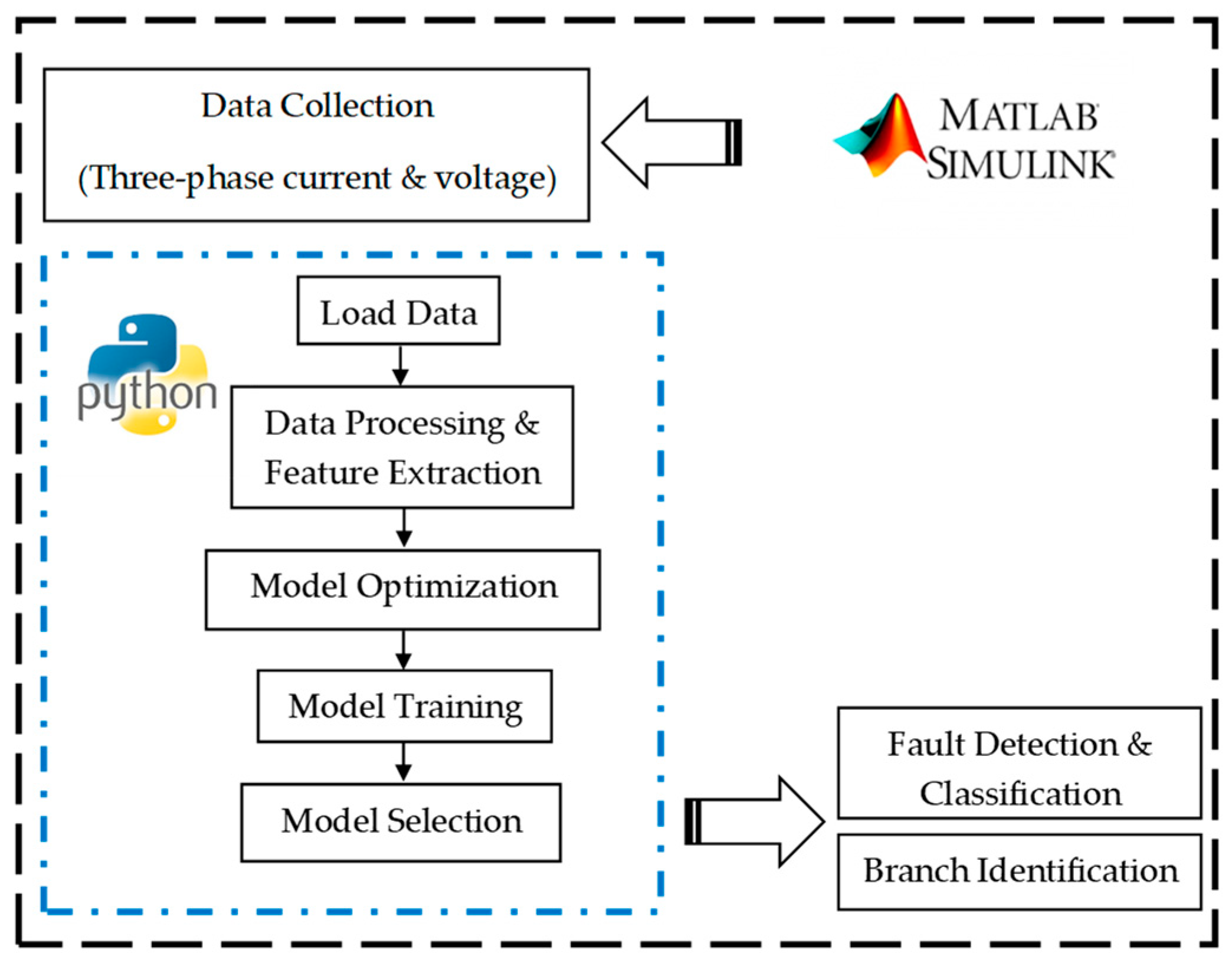
• High-resolution data collection: MATLAB/Simulink is used to generate realistic high-sampling-frequency voltage and current waveform data. These data were collected under different scenarios such as different fault durations (sub-cycle and multi-cycle) and deploying dynamic loads to generate harmonics into waveforms.
• High fault impedances: Very few studies investigated incipient fault identification [10,11] or incipient fault location [12]. However, they did not consider high-impedance faults. The proposed method is capable of detecting, classifying, and identifying faults with impedances ranging from 0.01–100 Ω.
• A method for fault detection and identification: Eight supervised learning methods are used, and their performances are compared to find the best model for incipient fault detection. Moreover, a distinction between the faulty and non-faulty phases is achieved, thus identifying the fault type: single-phase (LG), two-phase (LL-LLG), or three-phase faults (LLLL-LLLG).
• A method for faulty branch identification: ML classifiers are used to define the faulty branch.
• Topology-independent: The proposed approach for fault detection, identification, and location are generalizable and applicable to different grid topologies. Particularly, the method can be trained in a specific grid topology and employed in a different one.

This paper is organized as follows: In the following section, an explication of intermittent fault characteristics and a developed method for fault detection, classification, and branch identification are provided. ML tools are described briefly in Section 3. In the fourth section, the results are presented and discussed. Finally, the conclusions are drawn in the last section.

2. Incipient Fault Definition and Simulation Approach

In this section, the characterization of the intermittent faults, simulation, and methods for fault detection, classification, and branch identification will be discussed.

2.1. Characterization of Intermittent Faults

Typical protection devices in distribution networks are configured to break a short circuit within hundreds of milliseconds up to a few seconds. Very-short-duration faults (in the sub-cycle up to several cycles range), therefore, remain undetected until the cable damage at the fault location is severe enough for a sustained short circuit current that triggers the protection device. These short-duration faults are referred to as intermittent faults. Regulatory reporting requires the classification of faults into non-supply-interruption incidents, where the compromised asset self-heals to a sufficient extent to allow the circuit to be re-energized, and supply interruption incidents, where the compromised asset needs service intervention. According to [1], faults in power systems can be categorized into three groups: pre-faults, temporary faults, and permanent faults. Among these faults, only permanent faults are damage-causing faults require maintenance. This paper will focus on pre-fault events which are an early indicator of permanent damage faults, referred to hereafter as intermittent faults. Based on our study, intermittent faults have the following specific characteristics:

• These faults typically start near the positive or negative peak of the voltage waveform and end at the zero-crossing of the current waveform;
• They are typically self-clearing;
• No overcurrent protective device operates because of the short duration and self-clearance;
• The frequency of intermittent fault occurrence increases over time until permanent failure occurs;
• They are precursors to permanent failures;
• Intermittent faults can have a high impedance, meaning that an arc voltage may be present [12].

The generated arc voltage waveform is similar to a square wave with a small transient one that occurs at each half-cycle. The arc voltage and the fault current are typically in phase [12]. As the faulty asset further deteriorates, many single-phase faults may develop into multi-phase intermittent faults before they turn into permanent faults. Most intermittent faults self-clear in less than one cycle or within four cycles [13]. Intermittent current peaks of faults with a duration of less than one cycle (often, in fact, less than ½ cycle) immediately self-clear, resulting in a current peak in the faulty phase. The current peak typically stops at the zero-crossing of the current waveform, as illustrated in Figure 1 and Figure 2. In Figure 1, intermittent faults are observed that occur over less than one cycle for the 0.01 Ω and 10 Ω fault impedances. It leads to a short-term current spike and a partial collapse of the phase-to-phase voltage. Figure 2 shows intermittent faults that affect current and voltage waveforms over multiple cycles. In both cases (sub-cycle and multi-cycle), the faults clear without activating the protection relays. It is worth mentioning that, with the increase of fault resistance, the amplitude of the current and voltage of the faulty situation approaches the amplitude of the current and voltage of the normal situation. Therefore, fault detection with higher impedances will be challenging because of the lower difference between the faulty and healthy current and voltage waveform amplitudes. Other intermittent faults, for example, those caused by tracking, may be present for several cycles before they self-clear. These multi-cycle intermittent faults are characterized by short-duration impulses or high-frequency oscillations that may occur once each half-cycle at the same instant as the faulted phase crosses zero.

2.2. Simulation

The IEEE 33 bus system in the radial and mesh configuration was modeled in the MATLAB–Simulink environment as shown in Figure 3. The IEEE 33 bus system represents a feeder in the MV distribution network consisting of 33 buses, 32 lines, and 4 branches. The nominal voltage at the substation is 12.66 kV, and the total load is 3.715 MW and 2.3 MVar. The line frequency for the network is considered to be 50 Hz. The simulation was performed for different single- and three-phase electrical faults at different places of four branches at different times as shown in Figure 3. To simulate the most realistic conditions, five different effects were identified and considered in this study:

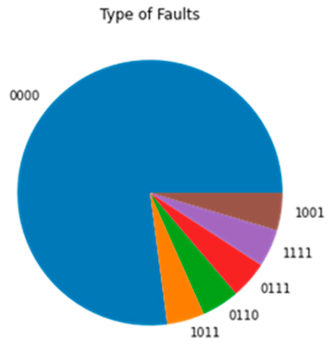
• Fault types: All possible electrical faults are considered in this research; LG, LL, LLG, LLL, and LLLG.
• Fault resistance: As explained in the motivation, very few studies were reported in the literature that covers HIFs in distribution systems. In this case, nine different fault impedances were investigated: 0.01, 1, 3, 5, 10, 25, 50, 75, and 100 Ω, covering the full spectrum of faults, both low- and high-impedance ones.
• Fault duration: Two different fault durations were considered, 5 ms and 50 ms, to represent sub-cycle and multi-cycle intermittent faults.
• Harmonics: To generate the harmonics in current and voltage waveforms, non-linear loads were used in this simulation.
• Imbalanced network: An imbalanced three-phase system is considered in this study to distinguish between LLL and LLLG.

The individual line current and voltage for each phase in the three-phase system were measured, employing the three-phase V-I measurement block at several buses in the feeder. These voltage and current waveforms were collected from radial and mesh networks to use for different objectives of the study as will be discussed later. Figure 1 and Figure 2 are showing the current and voltage waveforms of intermittent failure over sub-cycles and multi-cycles for the 0.01 Ω and 10 Ω fault impedances. These results show that:

• Faults have a more significant impact on current than voltage waveforms.
• When fault impedance increases, the amplitude of the fault current will reduce and be closer to the regular current waveforms. As a result, it is more difficult to detect these faults.
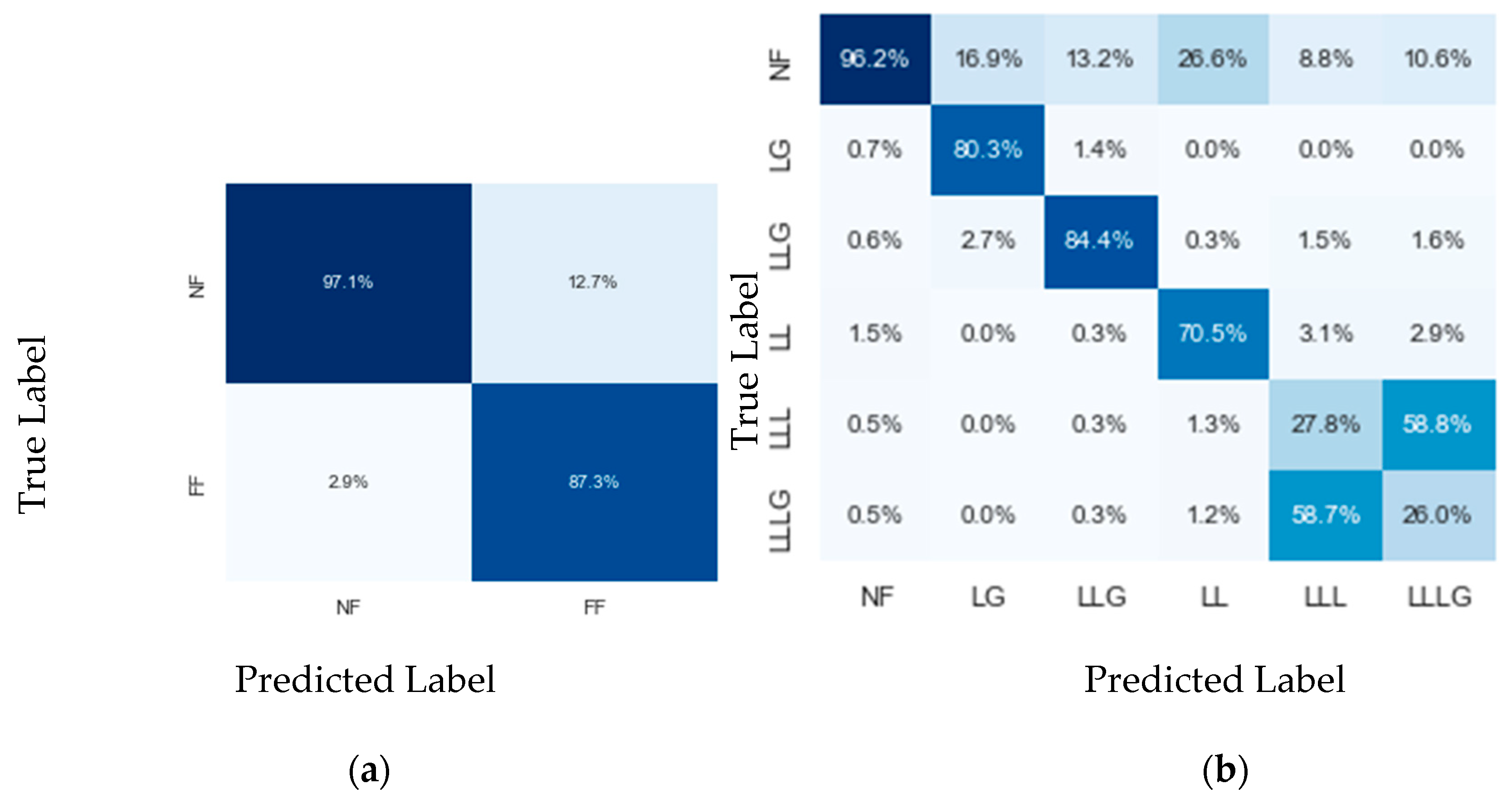
• Current and voltage waveforms for LLL and LLLG are close to each other. Therefore, it is not easy to distinguish them from each other, especially for multi-cycle faults.

Figure 3. IEEE 33-bus distribution system: (a) radial configuration; and (b) mesh configuration.

Figure 3. IEEE 33-bus distribution system: (a) radial configuration; and (b) mesh configuration.

2.3. Fault Detection and Identification

In this research, eight supervised learning methods were used to detect and identify intermittent electrical faults. For this reason, the collected current and voltage waveforms from the simulation are fed to each learning method for classifying the inputs into a set of desired categories. For fault detection, the outputs are either 1, which signifies the presence of a distinct type of fault, or 0, for the absence of a particular fault type. Each of these intermittent faults has an identical pattern. To identify the type of fault, the output of the algorithm considers the labeling for each fault as it is defined in

Table 1. Labeled faults for fault-type identification.

Fault Type	Output
	G	C	B	A
No fault	0	0	0	0
LG	1	0	0	1
LL	0	0	1	1
LLG	1	0	1	1
LLL	0	1	1	1
LLLG	1	1	1	1

. The data distribution for fault classification is shown in Figure 4 for both datasets (radial and mesh). This figure shows a balanced distribution, which helps to improve the classification result [14].

2.4. Branch Identification

To identify the faulty branch, the algorithm is trained to distinguish between five labels (0–4) which are presenting branch numbers. The collected current and voltage waveforms are used as inputs for the classifier.

2.5. Training

For eight selected classifiers, the algorithm is trained to minimize the cross-entropy loss of the training dataset. In addition, to optimize the structure of the algorithm, all the hyperparameters are optimally selected using HalvingGridsearchCV. The search strategy of HalvingGridsearchCV starts evaluating all the candidates with a small number of resources and iteratively selects the best candidates, using more and more resources [15].

2.6. Evaluation and Model Selection

The proposed method is designed to solve three different tasks: fault detection, classification, and identification of the faulty branch. For these tasks, as they are standard classification problems, two standard metrics are considered: accuracy and error. Moreover, the training time was measured and compared for all ML models. The error or mean squared error (MSE) is defined as the mean or average of the square of the difference between the actual and estimated values:

$$\mathrm{E}\mathrm{r}\mathrm{r}\mathrm{o}\mathrm{r}=\mathrm{M}\mathrm{S}\mathrm{E}=\frac{1}{\mathrm{N}}{\sum }_{\mathrm{i}}^{\mathrm{N}}{(Y_{true}-Y_{pre})}^2.$$

(1)

where N is the number of collected data, $Y_{true}$ is the actual value, and $Y_{pre}$ is the predicted value by the model. And the accuracy of the method is defined below:

$$\mathrm{A}\mathrm{c}\mathrm{c}\mathrm{u}\mathrm{r}\mathrm{a}\mathrm{c}\mathrm{y}=\frac{t_p+t_n}{t_p+t_n+f_p+f_n}$$

(2)

where $t_p$ is the number of true positives—i.e., for branch identification, it is the number of times that a faulty branch is correctly identified; $t_n$ is the number of true negatives—i.e., the number of times a healthy branch is correctly identified; and $f_p/f_n$ is the number of false positives/negatives, i.e.—the number of times a faulty/healthy branch is identified but the feeder is healthy/faulty.

3. ML Tools

As noted previously, supervised ML methods are used for fault detection, classification, and branch identification in this paper. The section that follows briefly describes the types of ML tools that are used for these purposes.

3.1. Linear Regression (LiRe)

LiRe assumes a linear relationship between the input and output. It is a very simple model and easy to implement for regression problems. Because LiRe oversimplifies real-world problems by assuming a linear relationship between variables, it is not recommended for most practical applications [16].

3.2. Logistic Regression (LoRe)

LoRe is a classification procedure that assigns observations to a discrete set of classes. The logistic sigmoid function is used to convert the output of LoRe to return a probability value [17].

3.3. Multi-Layer Perceptron (MLPC)

MLP is the most common type of feed-forward artificial neural network (ANN). MLP is made up of three layers: the input layer, the hidden layer, and the output layer. The hidden layer receives a dataset from the input layer. The data are processed by the hidden layer using the activation function, and the desired output is then delivered to the output layer [2].

3.4. Naive Bayes (NB)

The Bayes theorem underpins the NB classifier. It has a background in probabilistic classifiers. Because these classifiers are simple to implement, they are commonly employed in ML classification. The Bayes theorem is given by (3) [16]:

$$\mathrm{P}\left(\mathrm{A}|\mathrm{B}\right)=\frac{\mathrm{P}\left(\mathrm{B}|\mathrm{A}\right)\mathrm{P}\left(\mathrm{A}\right)}{\mathrm{P}\left(\mathrm{B}\right)}.$$

(3)

where P(A|B) is the probability of event A occurring, given that event B has occurred. P(B|A) is the probability of event B occurring, given that event A has occurred, and P(A) is the probability of event A.

3.5. Decision Tree (DT)

DT is a strong tool in supervised learning algorithms that may be utilized for both classification and regression applications. It creates a flowchart-like tree structure, with each internal node representing a test on an attribute, each branch representing a test outcome, and each leaf node (terminal node) holding a class label. It is built by iteratively splitting the training data into subsets depending on attribute values until a stopping requirement, such as the maximum depth of the tree or the minimum number of samples needed to divide a node, is met. During training, the DT algorithm chooses the appropriate attribute to split the data depending on a metric such as entropy or gini impurity, which quantifies the degree of complexity of the data [16].

3.6. KNN

KNN is known as a non-parametric, supervised learning classifier, which uses proximity to make classifications or predictions about the grouping of an individual data point. While it can be used for either regression or classification problems, it is typically used as a classification algorithm, working off the assumption that similar points can be found near one another. To classify the new data point, KNN normalizes the numeric data and defines the distance between the new data point and all training data points. Then, it sorts the distance and finds the closest K data points. Finally, it classifies the new data point based on the nearest K points. K is the number of neighbors that should be defined by the user. The value of K is very crucial. A small value of k may result in overfitting, whereas a large value of k may result in underfitting [18]. Overfitting occurs when a model predicts the training data too well but performs poorly when new data are included.

3.7. GB

GB was proposed by Jerome Friedman in 2001 because he believed that with small steps it is possible to predict better with a dataset that is being tested [16]. GB is used for regression and classification problems that produce a prediction model in the form of an ensemble of weak prediction models. Such models are popular due to their ability to properly classify datasets. In most cases, decision trees are used to generate models for the GB classifiers.

3.8. Random Forest (RF)

RF is a popular ML technique developed by Leo Breiman and Adele Cutler that combines the output of numerous decision trees to produce a single conclusion. Its ease of use and adaptability, as it covers both classification and regression problems, has propelled its adoption [19].

4. Results and Discussion

The IEEE 33 bus system is a four-branch feeder as shown in Figure 3. All single-phase and three-phase faults are applied to take into account all the previously described constraints between two specified buses as indicated in Figure 3. Fault impedances are in a range of 0.01 Ω to 100 Ω (0.01, 1, 3, 5, 10, 25, 50, 75, and 100) with 5 ms and 50 ms durations. A simulation has been performed for the radial and mesh network configurations. Then, voltage and current waveforms were collected from buses 10, 20, 23, and 30 with a sampling frequency of 10 kHz for both simulations (radial and meshed). These data are used as inputs (see Figure 5) for different objectives (fault detection, classification, and branch identification). Each dataset consists of 1,859,832 labeled data points. The outputs are defined based on each objective as described in Section 2. The randomized training set comprised two-thirds of the collected data, whilst one-third was retained as an unseen test set. LiRe, LoRe, MLPC, NB, DT, KNN, RF, and GB have been trained on both datasets for all three cases.

Tuning the hyperparameters for the selected algorithm for each case was a big challenge in terms of computation time. Therefore, for LiRe and LoRe, the default hyperparameters from scikit-learn were considered in all three objectives. For the other models, all the hyperparameters were optimally selected for each model before training using HalvingGridsearchCV. The hyperparameters are represented in

Table 2. Hyperparameters for ML classifiers.

Model	Model Hyperparameters
	Fault Detection	Fault Classification	Branch Identification
MLP	solver = ‘adam’, alpha = 1e-5, hidden_layer_sizes = (5, 2), random_state = 1,max_iter = 700	solver = ‘adam’, alpha = 1e-5, hidden_layer_sizes = (10, 6), random_state = 1,max_iter = 1500	solver = ‘adam’, alpha = 1e-5, hidden_layer_sizes = (10, 6), random_state = 1,max_iter = 1500
NB	var_smoothing = 1.2328467394420635e-09	var_smoothing = 8.111308307896856e-09	var_smoothing = 2.310129700083158e-07
DT	criterion = ‘entropy’, max_depth = 20, min_samples_leaf = 5, random_state = 42	criterion = ‘entropy’, max_depth = 20, min_samples_leaf = 5, random_state = 42	criterion = ‘entropy’, max_depth = 20, min_samples_leaf = 5, random_state = 42
KNN	metric = ‘manhattan’, n_neighbors = 2, weights = ‘distance’	metric = ‘manhattan’, n_neighbors = 5, weights = ‘distance’	metric = ‘manhattan’, n_neighbors = 5, weights = ‘distance’
RF	max_depth = 6, min_samples_leaf = 2, min_samples_split = 5, n_estimators = 56, bootstrap = ‘False’,max_features = ‘sqrt’	max_depth = 6, min_samples_leaf = 1, min_samples_split = 5, n_estimators = 72, bootstrap = ‘False’,max_features = ‘sqrt’	max_depth = 6, min_samples_leaf = 1, min_samples_split = 2, n_estimators = 41, bootstrap= True, max_features= ‘sqrt’
GB	n_estimators = 100, learning_rate = 1.0, max_depth = 20	n_estimators = 50, learning_rate = 1.0, max_depth = 20	n_estimators = 100, learning_rate = 0.1, max_depth = 20, random_state = 0

.

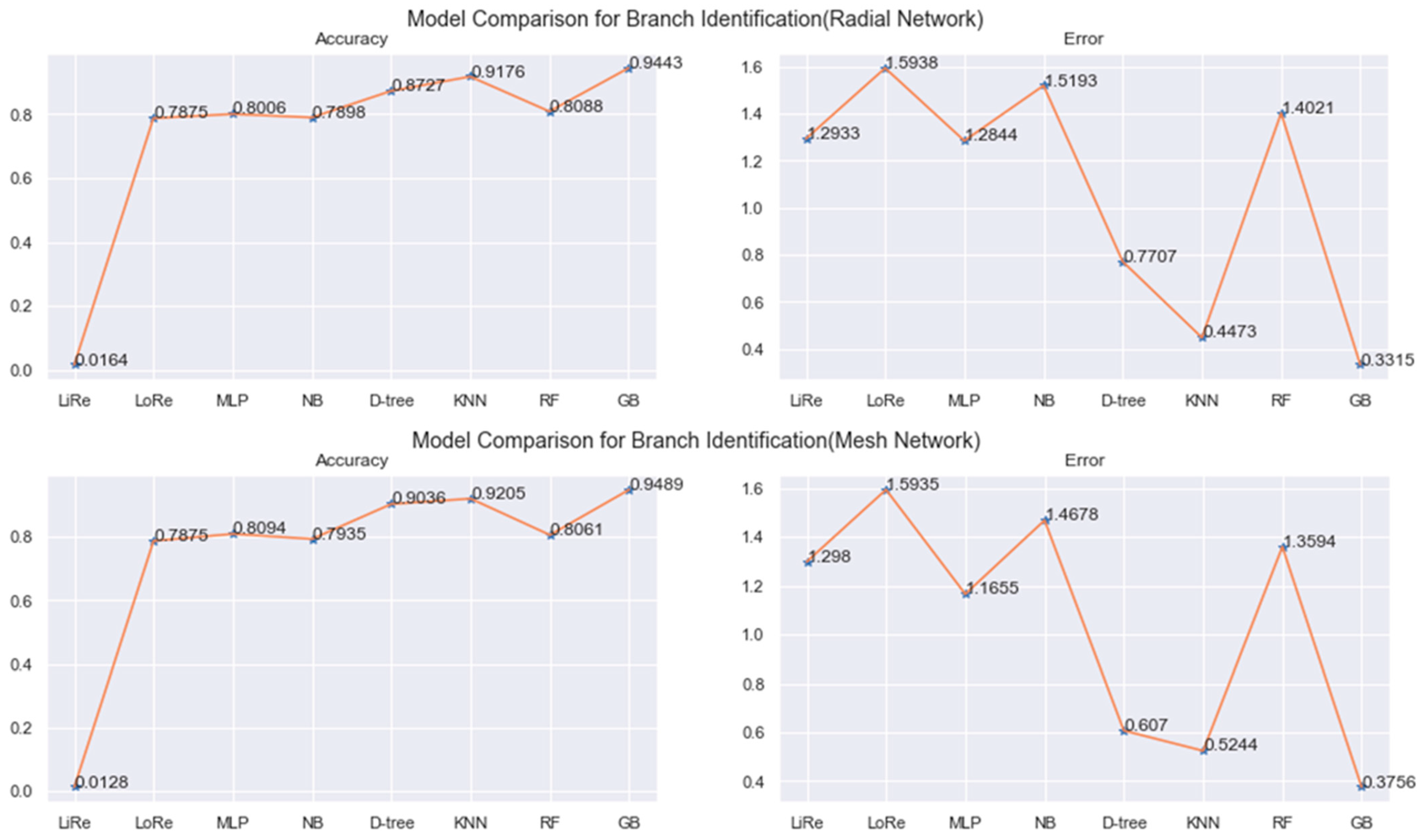
4.1. Branch Identification

A comparison between the accuracy and MSE for branch identification has been performed and is shown in Figure 6. Based on this result, KNN obtained an accuracy of 91.8% and 92% when identifying the faulty branch in the mesh and radial network while GB achieved 94.4% and 94.9% in these cases. Confusion matrices for branch identification using GB are represented in Figure 7. These matrices show that faulty branches can be detected clearly.

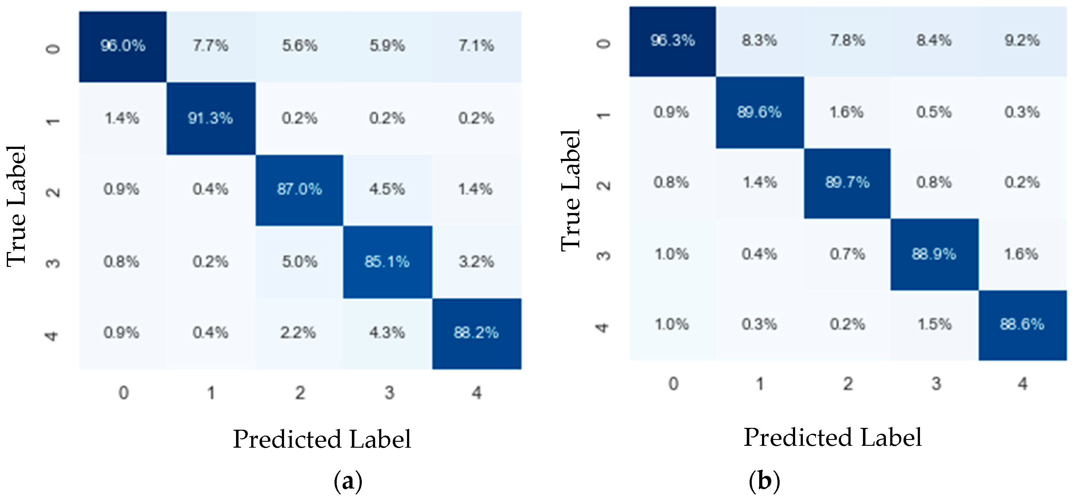
4.2. Fault Detection and Fault-Type Identification

Comparison results based on the accuracy and the error for fault detection and fault-type identification are represented in Figure 8. This figure shows the best accuracy and lowest MSE achieved by GB and KNN for intermittent fault detection. The GB achieved a 0.948 and 0.949 accuracy for the radial and mesh network datasets, meaning that nearly 95% of the faults were correctly detected. After GB, KNN obtained 94.4% and 93.9% accuracy. Moreover, KNN has the best accuracy for fault classification with an accuracy of 87.8% for both the radial and mesh network topologies. It should be mentioned that, because of the long computation time, the default hyperparameters of the GB model were used for fault classification as well. A potential improvement may be possible by GB using the optimal parameters.

The confusion matrices in Figure 9 and Figure 10 show all five faults can be identified using KNN. The confusion matrices show the classification performance for LLL and LLLG is relatively low. That is because the voltage and current waveforms for the symmetrical faults LLL and LLLG are similar to each other, which makes it difficult to distinguish between these two symmetrical fault types. Therefore, it is expected that the classification results will be improved by ignoring LLL faults. The LLL fault is balanced, which means the system remains balanced after the fault occurs. This type of fault happens when two conductors of a three-phase system break and fall on the conductor of the third line. In reality, this kind of symmetrical fault rarely occurs. Therefore, if the model can identify one or the other of these faults, it is a meaningful insight.

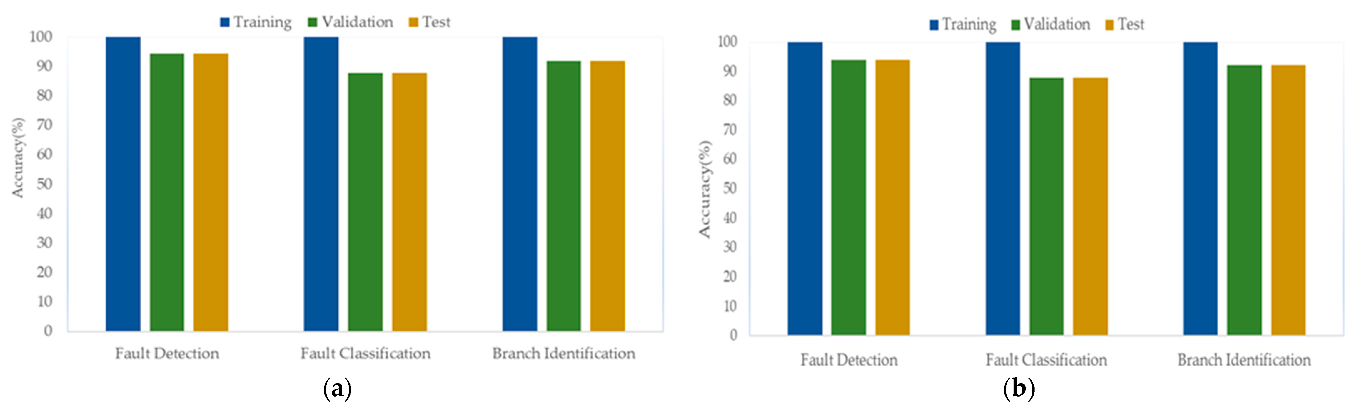
4.3. Performance Comparison

Overall, GB has the highest accuracy for fault detection and faulty branch identification. However, as shown in Figure 11, GB has a very high training time compared to the other models. The training time for fault-type identification takes up to 29,028.52 s. On the other hand, it is only 7.51 s for KNN.

4.4. Overfitting

Overfitting is one of the main problems of ML methods [20]. Overfitting causes models to perform well on training data but perform poorly on fresh data. The main factors for overfitting are the use of a small dataset or the complexity of the model. The datasets that are used in this study are quite big (1,859,832 labeled data points for each dataset). As discussed in the previous section, GB and KNN have the best performance in terms of high accuracy and low error compared to the other methods. However, KNN is much faster than GB and this makes it more suitable for real-time applications. The K value has an important impact on overfitting in the KNN model. For this reason, in this research, KNN hyperparameters including K are defined using optimization to avoid over- or underfitting.

To show that the KNN does not overfit, the performance of this method is compared with the training, validation, and test datasets. Therefore, the dataset is split into 70%, 20%, and 10% for training, testing, and validation, respectively. And the accuracy for all three objectives is calculated with the training, validation, and test data, and is shown in Figure 12. As can be clearly seen, the model does not overfit for fault detection, fault-type identification, and branch identification. This is because of a minor decrease in accuracy between the training and validation dataset, and validation and test dataset; this behavior is expected. The method always performs a little bit better in the datasets used for training, and minor variations between the datasets are expected because the data distribution in each dataset is slightly different [7].

4.5. Comparison with Literature Methods

Table 3. Comparison of case studies for fault detection methods.

Parameters	[6]	[7]	This Case Study
Grid voltage (kV)	0.4	0.4	12.66
Method	DNNs	GBT	GB, KNN
Fault types	LG, LLL	LG, LLL	LG, LLG, LLLG, LLL, LL
Accuracy	100	84.1-95.8	93.9–94.9
Sample frequency (kHz)	NA	NA	10
Fault characteristic	permanent	permanent	intermittent
Fault resistance (Ω)	0.1–1000	0.1, 0.5, 1, 3, 5, 7.5, 10, 30, 50, 75, 100, 300, 500, 750, 1000	0.01, 1, 3, 5, 10, 25, 50, 75, 100

,

Table 4. Comparison of case studies for fault identification methods.

Parameters	[5]	[21]	This Case Study
Grid voltage (kV)	11	22	12.66
Method	ANN	SVM, NN, DT	KNN
Fault types	LG, LLG, LLLG	LG, LLG, LLLG, LLL, LL	LG, LLG, LLLG, LLL, LL
Accuracy	84.5	83-97.6	87.8
Sample frequency (kHz)	NA	12.5	10
Fault characteristic	permanent	permanent	intermittent
Fault resistance (Ω)	LIF	LIF	0.01, 1, 3, 5, 10, 25, 50, 75, 100

and

Table 5. Comparison of case studies for branch identification methods.

Parameters	[6]	[7]	This Case Study
Grid voltage (kV)	0.4	0.4	12.66
Method	deep learning	GBT	GB, KNN
Fault types	LG, LLL	LG, LLL	LG, LLG, LLLG, LLL, LL
Accuracy	83.5	91.7-93.8	91.8-94.9
Sample frequency (kHz)	NA	NA	10
Fault characteristic	permanent	permanent	intermittent
Fault resistance (Ω)	0.1, 0.5, 1, 3, 5, 7.5, 10, 30, 50, 75, 100, 300, 500, 750, 1000	0.1, 0.5, 1, 3, 5, 7.5, 10, 30, 50, 75, 100, 300, 500, 750, 1000	0.01, 1, 3, 5, 10, 25, 50, 75, 100

present four studies that have been carried out on electrical fault detection, classification, and branch identification. [6,7] investigated LG and LLL fault detection and branch identifications using deep neural networks (DNNs) and gradient boosting trees (GBT). However, these faults are permanent and not intermittent. Moreover, in this paper, a range of LIFs and HIFs was investigated separately. In contrast, this paper considered a combination of all faults with low and high resistances with short and long durations. Fault-type identification studies have been carried out in [5,21] on an MV distribution network using ANN, support vector machines (SVMs), and DT. Although only low-impedance faults were investigated in these studies. It is important to note that, since the case studies are different, the accuracy differences between the methods cannot be strictly measured and this comparison is purely qualitative. In addition, most of the methods from the literature are proposed for permanent electrical faults, which differ significantly from intermittent faults.

5. Conclusions

This paper focuses on intermittent fault detection, classification, and faulty branch identification in distribution networks using ML methods. To define a fast and accurate model, eight popular ML algorithms were used to train two datasets collected from the simulation. To achieve realistic data, all the possible single- and three-phase electrical faults with a 5 ms and 50 ms duration and a range of impedances (0.01–100 Ω) were applied to four different places at different times in the IEEE 33 bus system with radial and meshed configurations. The training results on two datasets from the radial and meshed topology show that the GB and KNN models achieve a better performance in terms of accuracy and error. However, the computation time for the GB is very high. The main advantage of KNN is its very fast estimation and easy implementation, which, in turn, makes it implementable in real-time applications.

A high accuracy for intermittent fault detection and faulty branch identification was achieved using KNN. In addition, intermittent fault classification showed very promising results. In detail, KNN obtained an accuracy of 94.4% to 93.9% for intermittent fault detection for radial and mesh networks, an accuracy of 87.8% when identifying intermittent fault types for both topologies, and an accuracy of 91.8% and 92% when identifying the faulty branch in the mesh and radial network. The effects of LLL and LLLG on the voltage and current waveforms are close to each other, so it is not easy to separate them. That is why the accuracy of the intermittent fault-type identification is lower compared to the other objectives.

It should be noted that these results were obtained under all the restrictions that were used to collect the data. Moreover, because of the limited number of studies conducted on intermittent faults in distribution systems, there are no specific methods for this kind of fault detection or classification to compare with. In future research, the model will be tested with real-time data acquisition devices capable of collecting voltage and current waveforms at high sampling frequencies.

References

1. Roberts, D.; Lees, M. Foresight Project; EA Technology: Chester, UK, 2021. [Google Scholar]
2. Mamuya, Y.D.; Der, L.Y.; Shen, J.W.; Shafiullah, M.; Kuo, C.C. Application of machine learning for fault classification and location in a radial distribution grid. Appl. Sci. 2020, 10, 4965. [Google Scholar] [CrossRef]
3. Teimourzadeh, H.; Moradzadeh, A.; Shoaran, M.; Mohammadi, B.; Razzaghi, R. High impedance single-phase faults diagnosis in transmission lines via deep reinforcement learning of transfer functions. IEEE Access 2021, 9, 15796–15809. [Google Scholar] [CrossRef]
4. Bon, N.N.; Van, D.L. Fault identification, classification, and location on transmission lines using combined machine learning methods. Int. J. Eng. Technol. Innov. 2022, 12, 91–109. [Google Scholar] [CrossRef]
5. Shahriar, R.F.; Yeahia, S.; Omar, K.I.; Subrata, K.S. An Intelligent Approach of Fault Classification and Localization of a Power Transmission Line. In Proceedings of the 2019 IEEE International Conference on Power, Electrical, and Electronics and Industrial Applications (PEEIACON), Dhaka, Bangladesh, 29 November–1 December 2019; pp. 53–56. [Google Scholar]
6. Sapountzoglou, N.; Lago, J.; De Schutter, B.; Raison, B. A generalizable and sensor-independent deep learning method for fault detection and location in low-voltage distribution grids. Appl. Energy 2020, 276, 115299. [Google Scholar] [CrossRef]
7. Sapountzoglou, N.; Lago, J.; Raison, B. Fault diagnosis in low voltage smart distribution grids using gradient boosting trees. Electr. Power Syst. Res. 2020, 182, 106254. [Google Scholar] [CrossRef]
8. Baicong, S.; Hengxu, Z.; Fang, S. Machine Learning Based Fault Type Identification in the Active Distribution Network. In Proceedings of the 2019 IEEE 3rd Information Technology, Networking, Electronic and Automation Control Conference (ITNEC 2019), Chengdu, China, 15–17 March 2019; pp. 1330–1334. [Google Scholar]
9. Asman, S.H.; Ab Aziz, N.F.; Amirulddin, U.A.; Ab Kadir, M.Z.A. Transient fault detection and location in power distribution network: A review of current practices and challenges in Malaysia. Energies 2021, 14, 2988. [Google Scholar] [CrossRef]
10. Xiong, S.; Liu, Y.; Fang, J.; Dai, J.; Luo, L.; Jiang, X. Incipient fault identification in power distribution systems via human-level concept learning. IEEE Trans. Smart Grid 2020, 11, 5239–5248. [Google Scholar] [CrossRef]
11. Zhang, C.; Song, N.; Li, Y. Incipient fault identification of distribution networks based on feature matching of power disturbance data. Electr. Eng. 2021, 103, 2447–2457. [Google Scholar] [CrossRef]
12. Herrera-Orozco, A.R.; Bretas, A.S.; Orozco-Henao, C.; Iurinic, L.U.; Mora-Flórez, J. Incipient fault location formulation: A time-domain system model and parameter estimation approach. Int. J. Electr. Power Energy Syst. 2017, 90, 112–123. [Google Scholar] [CrossRef]
13. Lukowicz, M.; Rebizant, W.; Kereit, M. New approach to intermittent earth fault detection with admittance criteria. Int. J. Electr. Power Energy Syst. 2020, 123, 106271. [Google Scholar] [CrossRef]
14. Hojabri, M.; Kellerhals, S.; Upadhyay, G.; Bowler, B. IoT-based PV array fault detection and classification using embedded supervised learning methods. Energies 2022, 15, 2097. [Google Scholar] [CrossRef]
15. Scikit-Learn. Available online: https://scikit-learn.org/ (accessed on 24 March 2023).
16. GeegkforGeeks. Available online: https://www.geeksforgeeks.org/ (accessed on 28 July 2023).
17. Towards Data Science. Available online: https://towardsdatascience.com/introduction-to-logistic-regression-66248243c148 (accessed on 28 July 2023).
18. Codecademy. Available online: https://www.codecademy.com/learn/machine-learning-k-nearest-neighbors/modules/knn-classification-course/cheatsheet (accessed on 28 July 2023).
19. IBM. What Is Random Forest? Available online: https://www.ibm.com/topics/random-forest (accessed on 28 July 2023).
20. Lago, J.; Ridder, F.D.; Vrancx, P.; Schutter, B.D. Forecasting day-ahead electricity prices in Europe: The importance of considering market integration. Appl. Energy 2018, 211, 890–903. [Google Scholar] [CrossRef]
21. Moloi, K.; Davidson, I. High impedance fault detection protection scheme for power distribution systems. Mathematics 2022, 10, 4298. [Google Scholar] [CrossRef]
Figure 1. Current and voltage waveforms of intermittent sub-cycle faults: (a) 0.01 Ω fault impedance; and (b) 10 Ω fault impedance.
Energies 16 06023 g001
Figure 2. Current and voltage waveforms of intermittent multi-cycle faults: (a) 0.01 Ω fault impedance; and (b) 10 Ω fault impedance.
Energies 16 06023 g002
Figure 4. Distribution of labeled data for fault-type identification.
Energies 16 06023 g004
Figure 5. ML process for fault detection, classification, and branch identification.
Energies 16 06023 g005
Figure 6. ML model comparison for branch identification.
Energies 16 06023 g006
Figure 7. Confusion matrices for branch identification using GB: (a) radial network; and (b) mesh network. The elements on the diagonal indicate the percentage of fault locations that were attributed to the correct branch, whereas the off-diagonal elements indicate the percentage of fault locations that were attributed to the respective incorrect branch.
Energies 16 06023 g007
Figure 8. Model comparison based on accuracy and error: (a) fault detection in the radial network; (b) fault detection in the mesh network; (c) fault-type identification in the radial network; and (d) fault-type identification in the mesh network.
Energies 16 06023 g008
Figure 9. Confusion matrices for radial network dataset: (a) detection using GB model; and (b) classification using KNN model.
Energies 16 06023 g009
Figure 10. Confusion matrices for mesh network dataset: (a) detection using GB model; and (b) classification using KNN model.
Energies 16 06023 g010
Figure 11. Comparison of ML models’ training time.
Energies 16 06023 g011
Figure 12. Accuracy for three objectives for the training, validation, and test datasets: (a) radial network; (b) mesh network.
Energies 16 06023 g012