Seismic Characterization of the Blue Mountain Geothermal Field

Abstract

Subsurface characterization is crucial for geothermal energy exploration and production. Yet hydrothermal reservoirs usually reside in highly fractured and faulted zones where accurate characterization is very challenging because of low signal-to-noise ratios of land seismic data and lack of coherent reflection signals. We perform an active-source seismic characterization for the Blue Mountain geothermal field in Nevada using active seismic data to reveal the elastic medium property complexity and fault distribution at this field. We first employ an unsupervised machine learning method to attenuate groundroll and near-surface guided-wave noise and enhance coherent reflection and scattering signals from noisy seismic data. We then build a smooth initial P-wave velocity model based on an existing magnetotellurics survey result, and use 3D first-arrival traveltime tomography to refine the initial velocity model. We then derive a set of elastic wave velocities and anisotropic parameters using elastic full-waveform inversion, and obtain PP and PS images using elastic reverse-time migration. We identify major faults by analyzing the variations of seismic velocities and anisotropy parameters, and reveal mid- to small-scale faults by applying a supervised machine learning method to the seismic migration images. Our characterization reveals complex velocity heterogeneities and anisotropies, as well as faults, with a high spatial resolution. These results can provide valuable information for optimal placement of future injection and production wells to increase geothermal energy production at the Blue Mountain geothermal power plant.

1. Introduction

Geothermal energy plays an important role in renewable energy production in the United States and around the world. In the U.S., most of the geothermal reservoirs reside in the western continental states and Hawaii. The Blue Mountain geothermal field is a hydro-geothermal system located on the western flank of Blue Mountain in the Humboldt County of Nevada at an elevation of approximately 1350 m above the sea level. The Blue Mountain geothermal field was discovered as a blind geothermal reservoir enabled by a connected fracture network [1,2,3]. Lack of recent volcano activities in this region suggests that it is not heated by upper-crustal magmatism. Geothermal drilling has unveiled relatively high geothermal flow rates and temperatures (>190 °C) at depths of approximately 600 to 1070 m below the ground surface [4]. A geothermal power plant, the Faulkner I Energy Generation Facility, was developed in this geothermal field, and was commissioned in 2009 with an installed capacity of 49.5 MW and a net production of 38 MW.

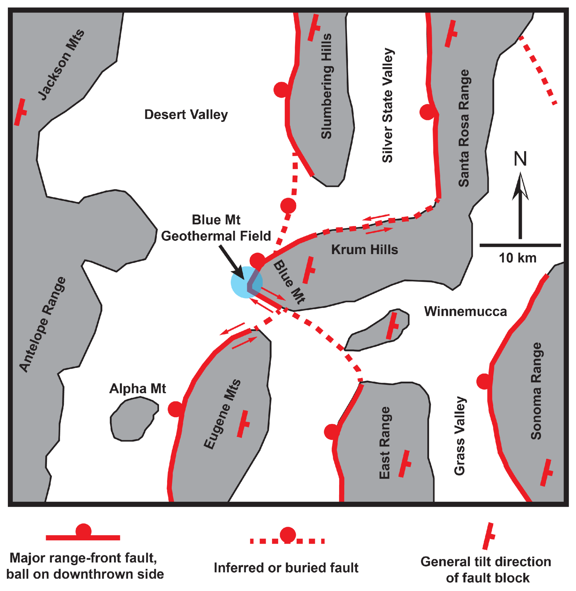
The regional geology and conceptual geological model around the Blue Mountain geothermal field has been well studied by [1,3,5]. Figure 1 displays the regional geology and particularly major faults in the Blue Mountain geothermal field area. Geologically, Blue Mountain is a faulted Triassic meta-sedimentary unit, spanning approximately 8 km long and tilting eastward. It sits between the Eugene Mountains and Slumbering Hills and is bounded by Desert Valley at the west. The Blue Mountain geothermal field, based on the current regional geology study, lies above the intersection between a regional NNE- to ENE-striking, west-dipping normal-sinistral fault system. In the vicinity of the geothermal field, there exists a localized WNW-striking, SW-dipping, normal-dextral fault on the southwest flank of Blue Mountain [1]. The majority of the Blue Mountain fault system is considered as a result of the Miocene diorite dike intrusion into the Triassic meta-sediments that occurred at approximately 12 ma. The intrusion was later covered by the late Tertiary to Quaternary sediments [3]. Such a geological setting results in a very complicated strain or deformation distribution and connected fault system in our study region that spans 6.5 km in both WE and NS directions [2].

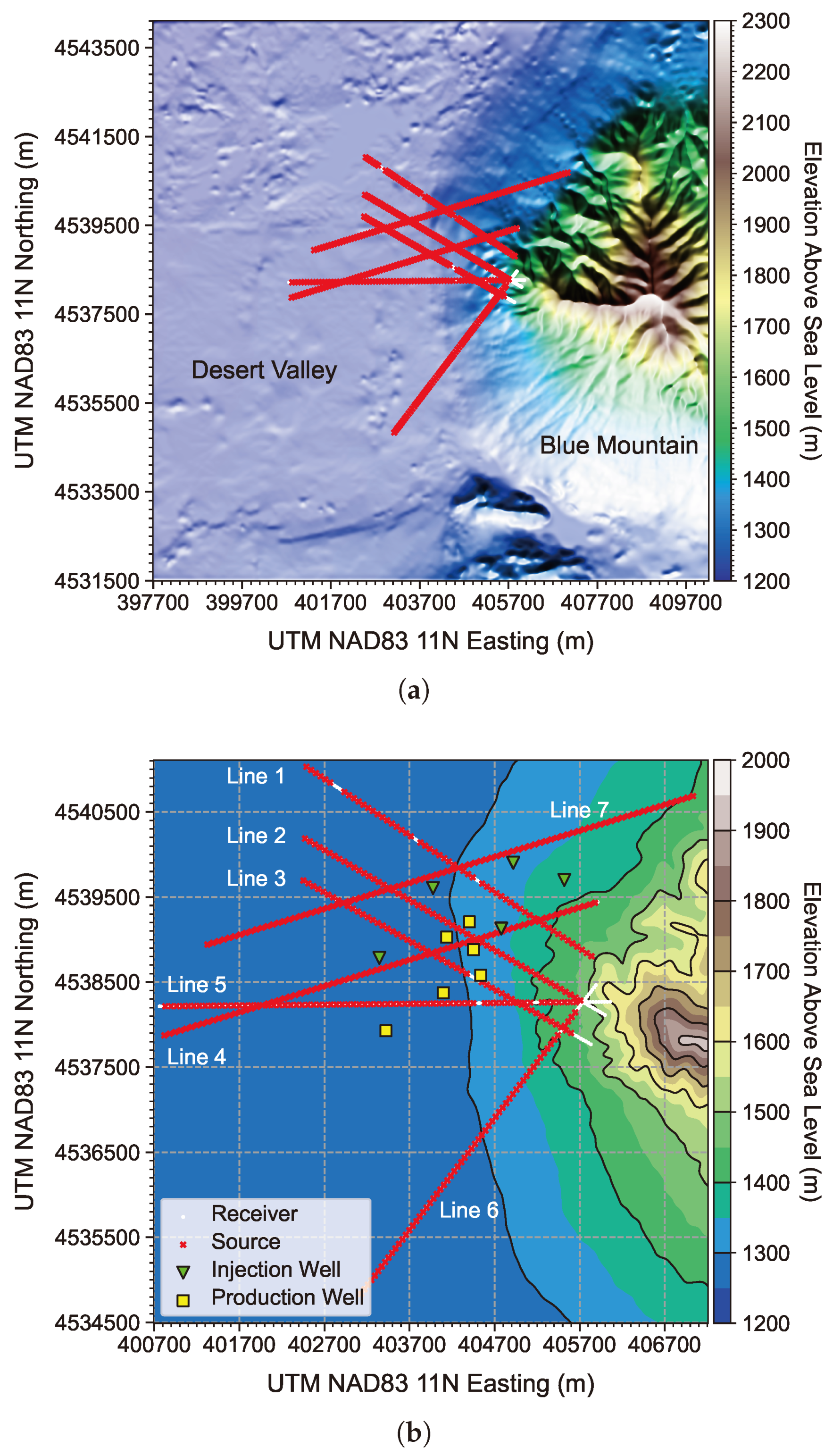
Multiple geophysical surveys have been conducted at the Blue Mountain geothermal field, including active and passive seismic, magnetotellurics (MT), and gravity surveys. In 2007, Cyrq/AltaRock acquired reflection seismic data along seven 2D seismic lines in this field, with source and receiver locations as displayed in Figure 2. The survey used 1-kg explosive sources buried approximately 5.2 m below the ground surface to prevent blowouts [6]. The lengths of these seismic survey lines vary from approximately 4 km to 6 km, and each contains 53 to 89 common-shot gathers, resulting in a total of 469 common-shot gathers. Each common-shot gather contains 117 to 179 receivers recording the z-component (or vertical component) of particle velocity field, resulting in a total of 68,613 traces. Along all the seven lines, the source interval is approximately 73.3 m (exactly 220 ft) while the receiver interval is approximately 36.7 m (exactly 110 ft). The Blue Mountain geothermal power plant is located on the east side of these lines, with several injection and production wells located in the intersection region among Lines 2, 3, 4 and 5 as displayed in Figure 2b. The seismic survey spans over an area with nontrivial elevation changes. For some of these seven lines, the maximum elevation difference is as high as 300 m, as indicated by the contours in Figure 2b.

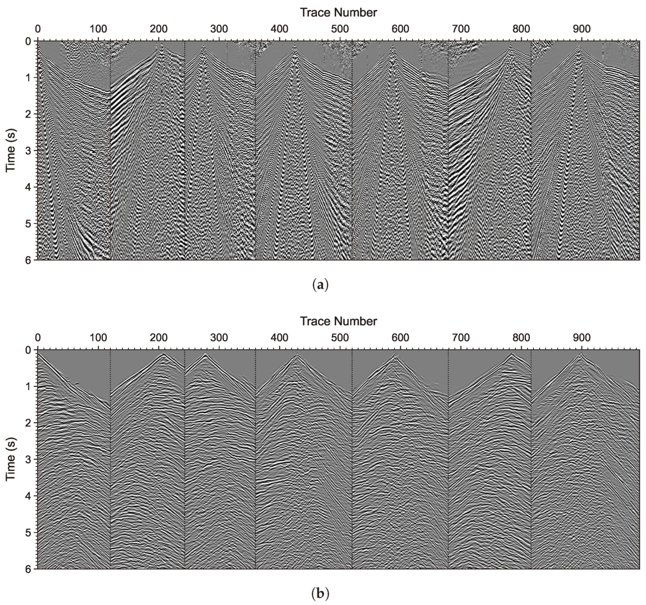
Figure 3 displays seven common-shot gathers randomly selected from the data, each from a different line. The data quality of these common-shot gathers is very poor—strongly-aliased groundrolls and near-surface guided waves dominate every common-shot gather, and no coherent reflection signals can be observed. The seismic data were processed by a seismic processing company with conventional seismic data processing tools, including random noise attenuation, ground-roll noise attenuation, deconvolution, and so on. The vendor then performed 2D refraction tomography to obtain a low-resolution P-wave velocity model for the shallow layers along each line, and performed Kirchhoff migration of the data [6]. 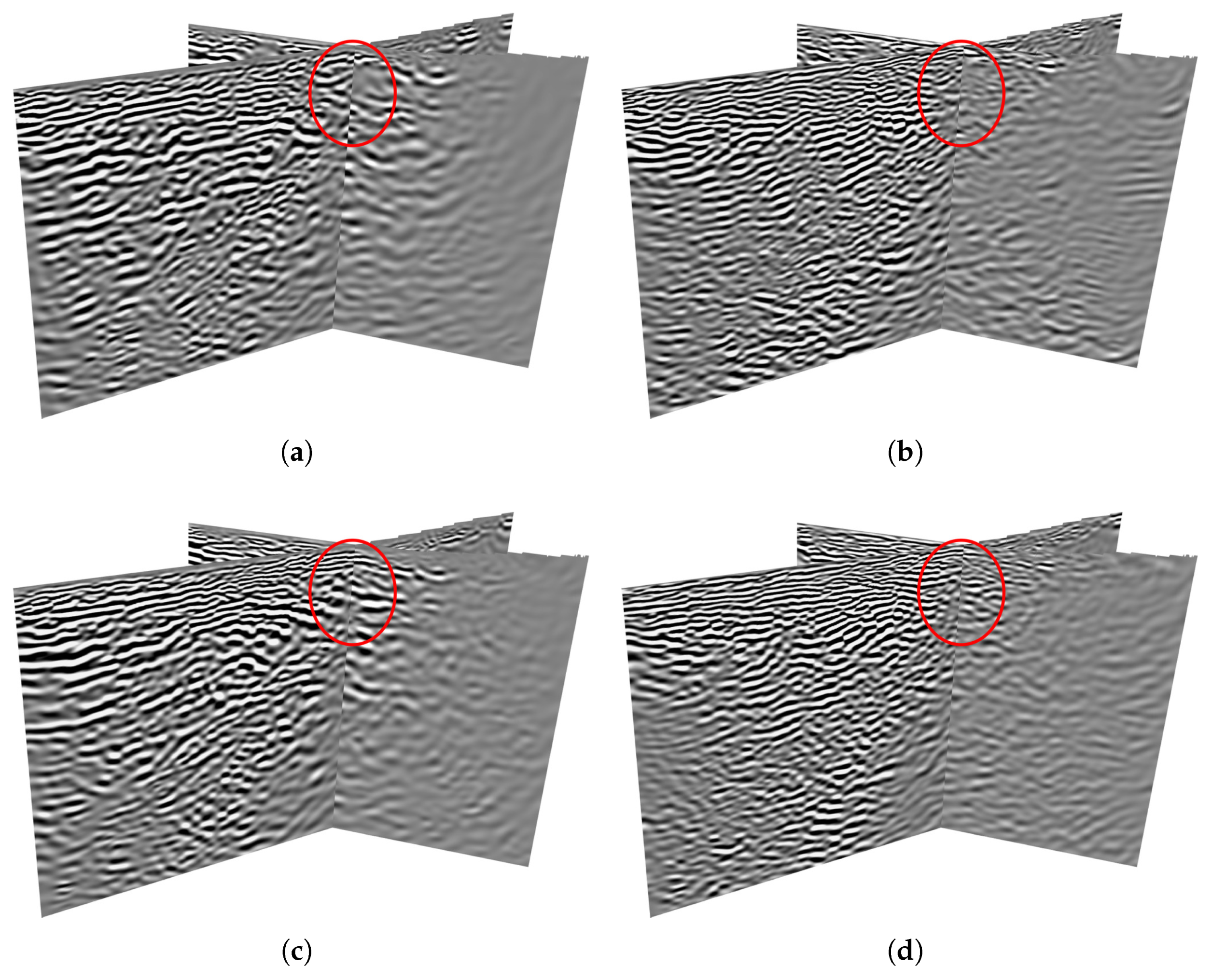However, a study based on these processed data and imaging results by [4] determined that because the vendor’s processed data (as displayed in Figure 4a) do not contain any visible reflection signals, the resulting migration images (Figure 5 in their paper) based on these data are possibly full of artifacts caused by the guided waves, instead of reflectors that resemble realistic subsurface structures. In addition, by mapping the traveltime tomography results to 3D, we also find inconsistencies at the intersections of seismic lines as displayed in Figure 4b. Therefore, in this study, we do not use these previously processed seismic data and picked traveltimes. Instead, we process the data using our own method and re-pick the first-arrival traveltimes from the data to perform traveltime tomography as detailed below.

For reliable seismic characterization of the Blue Mountain geothermal field, we aim to derive high-fidelity, high-resolution elastic medium properties and seismic migration images, and characterize the fault system using these models and images. To achieve this challenging goal based on the seven lines of active seismic data with low signal-to-noise ratios, we jointly use machine learning-based seismic data processing, full-waveform inversion, reverse-time migration, and machine learning-based fault detection.

Properly denoised seismic data are the basis for seismic imaging and inversion. The main issue plaguing the seven lines of Blue Mountain active seismic data, as shown in Figure 3 and Figure 4a, is that the aliased groundroll and near-surface guided wave are so strong that no reflection signals are visible. Groundroll noise attenuation is a challenging step in seismic data processing that is usually tackled by filter-based methods (e.g., [7,8]), adaptive attenuation (e.g., [9]), singular-value decomposition (e.g., [10]), and so on. We use an unsupervised machine learning (ML) method, namely the CycleGAN [11], to attenuate groundroll and near-surface guided wave noise in the Blue Mountain seismic data. CycleGAN is a type of generative adversarial network (GAN) [12] developed for unpaired image-to-image translation; it learns the “style” of images (i.e., their representative probability distribution) and performs translation of an image to the target style, e.g., real-world photo to Monet’s painting style. It relies on a generator to translate the input image to the target domain, and a discriminator to distinguish how well the target style has been learned by the NN compared to ground truth target styles. The idea of groundroll attenuation via GAN and CycleGAN have been explored and validated by [13,14], where the NN translates groundroll-contaminated data to data without groundroll. In this study, we use CycleGAN to learn and translate the Blue Mountain seismic data that are severely contaminated by groundroll and near-surface guided wave noise to data that contain only reflection signals. The target style is provided by simulating seismic data in a series of geological models with a random number of randomly oriented faults with an absorbing top surface (i.e., the synthetic data are free of surface wave signals). There are many approaches, including conventional and ML-based, that can perform groundroll noise attenuation, and the method we use here is just one of them. Validating and comparing these methods is beyond the scope this work.

We use first-arrival traveltime tomography (FATT) to derive a low-resolution velocity model for the Blue Mountain geothermal field. FATT seeks an optimal velocity model by matching the observed and synthetic fist-arrival traveltime. We implement the adjoint-state FATT [15,16] to perform refraction traveltime tomography because of its flexibility in handling complex heterogeneities. We carry out traveltime picking on the 68,613 traces using our in-house traveltime picking software.

With the denoised seismic data and the FATT-updated velocity model, we employ full-waveform inversion (FWI) [17,18,19] to obtain high-resolution subsurface medium parameter models based on the FATT result. FWI is known to be highly nonlinear and prone to the cycle-skipping issue (e.g., [20,21,22,23]). Many strategies and misfit functions have been developed to improve the robustness of FWI to cycle skipping and noise (e.g., [20,22,23,24,25,26,27]). In this study, we adopt a recently developed FWI misfit function based on optimal transport theory, the so-called graph-space optimal transport (GSOT) [23,28], to improve convergence and derive high-resolution models. Mathematical details and validations of GSOT for both synthetic and field seismic data have been well described by [23,28,29]. Note that in these studies, GSOT-FWI has been applied to synthetic and pressure data and proven to be robust to cycle skipping, but yet to be fully validated with elastic-wave data, particularly those collected by land seismic surveys that target deep structures. To investigate potential velocity anisotropy caused by fracturing and faulting at the Blue Mountain geothermal field, we perform two types of elastic FWI (EFWI): one based on an isotropic medium assumption where we invert for P- and S-wave velocities ($V_p$ and $V_s$), and the other based on anisotropic medium assumption where we invert for $V_p$, $V_s$, and two Thomsen parameters $\epsilon$ and $\delta$ [30]. For multi-parameter EFWI, there essentially exist parameter trade-offs (e.g., [26,31,32]), even for an EFWI that only inverts for $V_p$ and $V_s$ [33]. For the Blue Mountain seismic data, we apply a straightforward gradient-based method [34] parameterized in classical anisotropic parameters (i.e., Thomsen parameters) that does not involve Hessian or approximate Hessian (e.g., [32,35]) to update the elastic parameters, which, therefore, may be contaminated by parameter trade-offs. Properly eliminating parameter trade-offs for field seismic data may need more effort, including parameter decoupling by the Hessian and alternative forms of anisotropy parameterization [32,36]. However, that is beyond the scope of this paper.

Subsurface structural images can provide valuable information for placing geothermal injection and production wells. With the elastic medium property models derived using EFWI, we further use elastic reverse-time migration (ERTM) to obtain subsurface reflector images at the Blue Mountain geothermal field. ERTM was developed almost simultaneously with the acoustic counterpart [37,38], and is an effective tool for exploiting elastic wavefield information to form elastic (PP, PS, SP and SS) reflection images. Many strategies have been developed to overcome or alleviate challenges associated with ERTM (e.g., [39,40,41]). In this work, we perform ERTM to obtain the PP and PS images for the seven lines using a hybrid-domain dual-separation (i.e., a low-rank-based vector P-S wavefield separation and a Hilbert transform-based directional wavefield separation) [42,43,44] imaging condition. Details of this method can be found in [45].

Detecting faults is a key component of seismic characterization for the Blue Mountain geothermal field. Previous studies described the complex fault network near Blue Mountain [1,4,5] based on regional-scale geological models and low-resolution geophysical surveys, which therefore may miss small-scale faults developed in this field, particularly in the deep region. In recent years, ML-based automatic fault detection on seismic migration images (e.g., [46,47,48]) is becoming the state-of-the-art approach to automated fault detection because of its robustness and accuracy. We apply a recently developed ML-based fault detection algorithm based on nested residual U-Net [47] to elastic migration images, including PP and PS images, to automatically delineate faults beneath the seven seismic lines. Technical details of the fault detection method, including the network architecture and training/validation process, have been described by [47]. In addition to using an ML-based method to reveal mid- to small-scale faults, we also interpret the major fault in this area by visual inspection and hand picking. The interpretation along with the automatic fault detection results serve as the final results of our seismic characterization for the Blue Mountain geothermal field.

Figure 5 summarizes the aforementioned procedure of seismic characterization for the Blue Mountain geothermal field. We start from the MT survey resistivity model, raw seismic data, and the data acquisition geometry extracted from seismic data headers, to obtain the final products including inverted elastic parameter models, migration images, and fault maps. Our seismic characterization mainly uses an ML-based data processing method and prestack seismic imaging/inversion methods (EFWI, ERTM) to produce subsurface elastic parameter models and migration images. Therefore, conventional components of seismic data processing, such as velocity analysis, static correction, deconvolution, and so on, are not used in this workflow. In fact, we want to mitigate the impact of assumptions and approximations associated with these conventional processing steps in our study, and this study offers an experimental workflow to validate ML-based seismic data processing, seismic interpretation, and full-wavefield-based imaging and inversion for reliable seismic characterization at complex geothermal fields.

The rest of the paper is organized into four major sections. We first describe how we denoise the Blue Mountain seismic data to obtain coherent reflections using CycleGAN, and how to build a low-resolution initial $V_p$ model based on a previous MT survey model. We then describe how to perform 3D line-masked FATT using the traveltime picks. Following FATT, we describe how to perform 2D EFWI and analyze the high-resolution isotropic and anisotropic elastic medium property models. We then describe 2D ERTM results and obtain ML-detected fault maps along the seven lines. In the Discussion section, we share our point of view on the line intersection consistency issue and potential shortcomings of our seismic characterization for the Blue Mountain geothermal field. We summarize our work in the Conclusions section.

2. Seismic Data Denoising and Initial Model Building

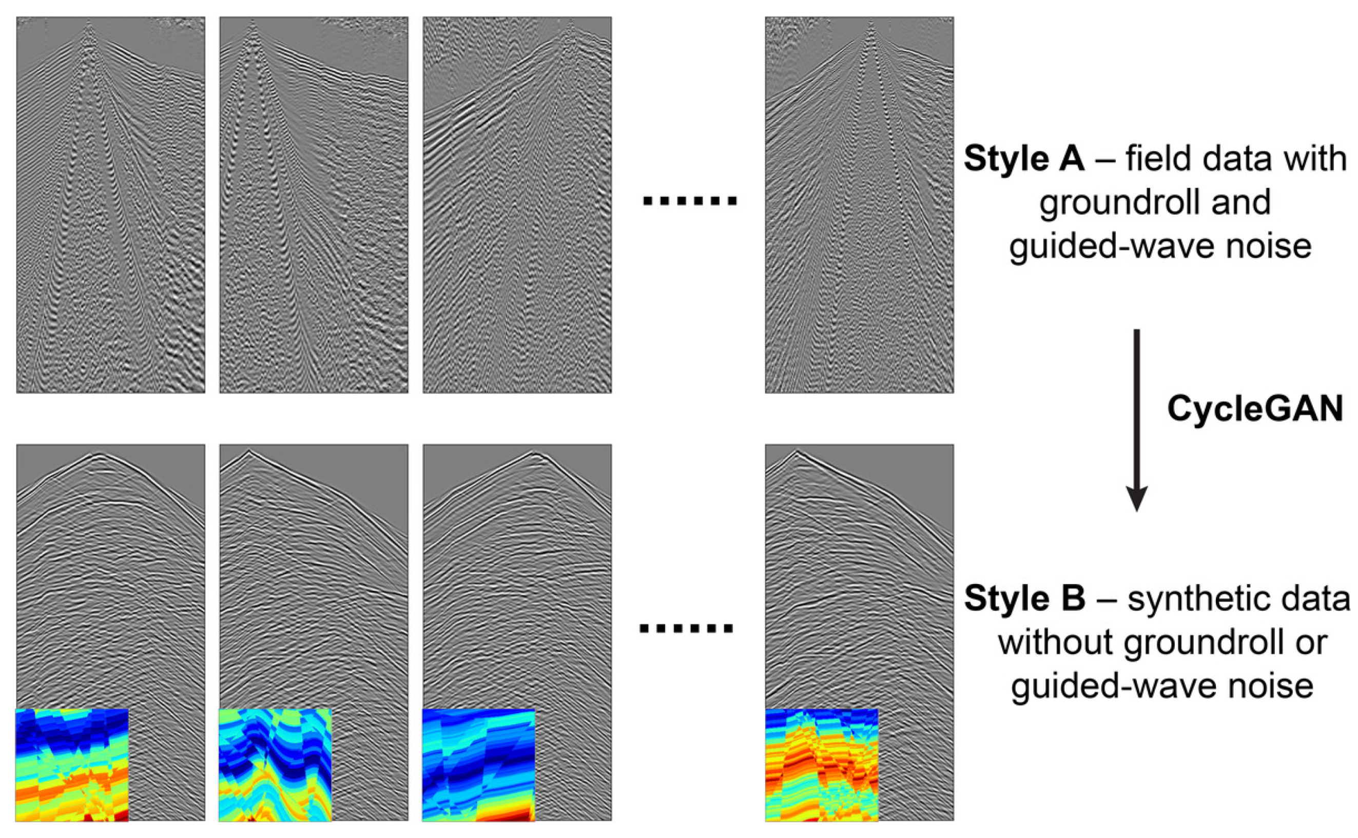
The basic mechanism of CycleGAN denoising is illustrated by Figure 6. “Style A” and “Style B” represent the source and the target image domain probability distributions, respectively. To form the target image domain, we first generate a total of 100 random faulted models using a similar strategy for generating random faults [47,48]. Each model contains a random number of randomly tilted faults, a random number of randomly curved reflectors, and random values of $V_p$, $V_s$, and density in the layers. We then generate a total of 460 synthetic common-shot gathers in these 100 randomly faulted models at 460 random source locations at the top surface (i.e., an average of 4.6 shots per model). The receivers for recording seismic waveforms are evenly distributed at the top surface. Because we have used perfectly matched layers at the top surface and the other three model boundaries, the resulting synthetic data do not contain surface waves or guided waves; meanwhile, they are sufficiently random in reflection patterns to form the target style (probability distribution) for CycleGAN to learn and to translate the Blue Mountain seismic data. We divide the 460 synthetic common-shot gathers into a training set with 400 gathers and a validation set with 60 gathers. We divide the Blue Mountain seismic data in a similar manner.

Our code is based on an open-source implementation of CycleGAN [49], with some modifications to the dataloader, input/output, and logging modules. The generators are based on ResNet [50] while the discriminator is composed of conventional convolutional layers, batch normalization layers, and rectified linear unit layers [51]. We train the CycleGAN implemented in PyTorch [52] with an Adam optimizer [53] for a total of 100 epochs, using a linear learning rate scheduler, a ${10}^{-4}$ initial learning rate for the generator and a ${10}^{-5}$ initial learning rate for the discriminator. We set a high weight of 500 for the cycle consistency loss and a relatively lower weight of 0.1 for the identity loss. 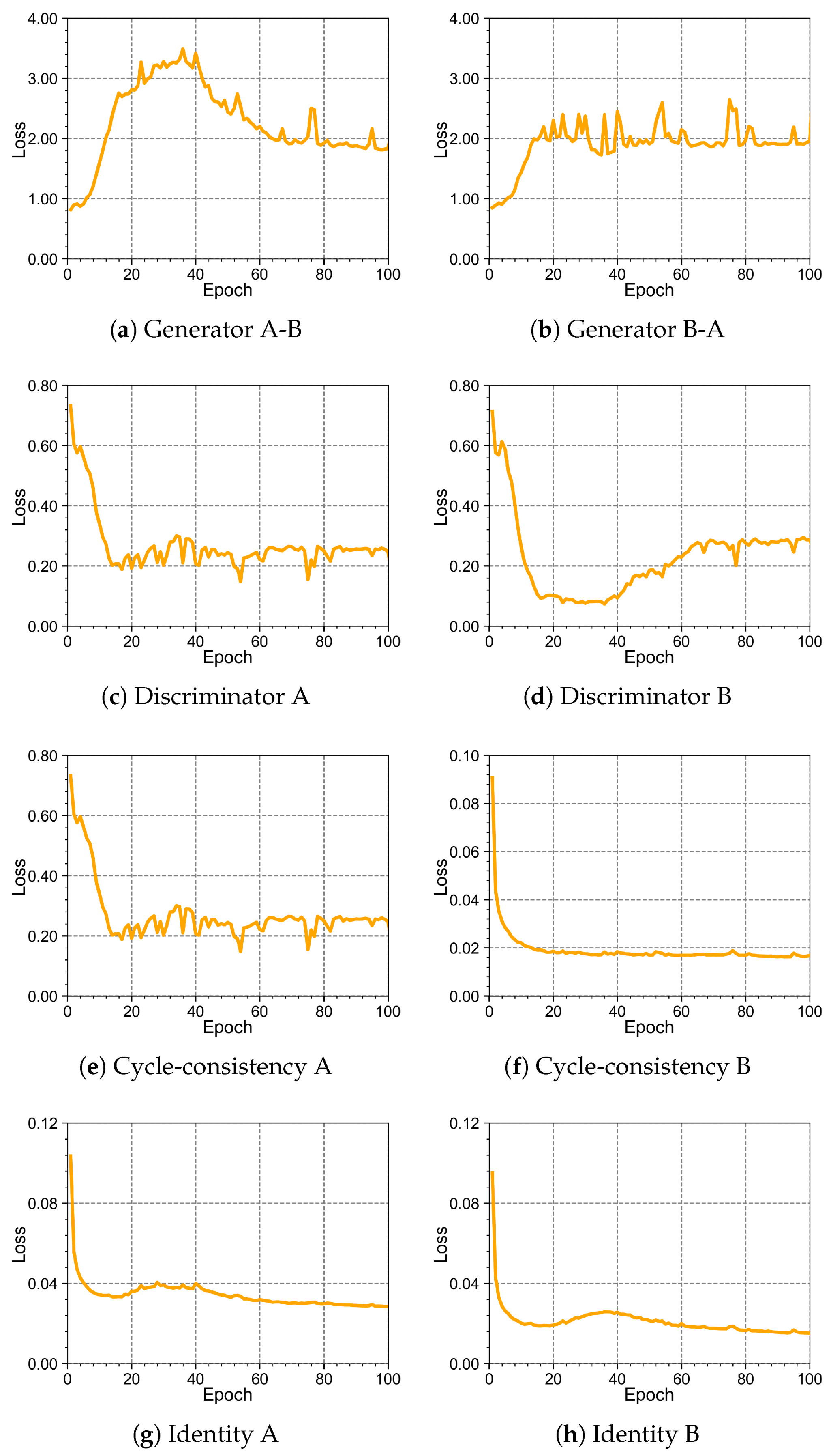Figure 7 displays the loss curves associated with the generators, the discriminators, the cycle consistency, and the identify losses. The definitions of these losses can be found in [11]; for brevity, we do not display the associated equations here. Note that we perform the style transfer from A (field data style) to B (synthetic data style). The generator A-B loss displayed in Figure 7a and the discriminator B loss displayed in Figure 7d show reasonable behaviors where, during the training, the generator generates more realistic fake images (denoised field data) that are more difficult for the discriminator to distinguish from real images (noise-free synthetic data). Meanwhile, both the cycle consistency and the identity losses decrease during training. After training, we apply the model to every common-shot gather of the Blue Mountain field seismic data. Figure 8a shows seven randomly selected common-shot gathers from the Blue Mountain seismic data after simple root-means-square (RMS) trace-by-trace balancing, while Figure 8b displays the denoised data corresponding to these seven common-shot gathers. We find that the CycleGAN attenuates most of the groundroll and near-surface guided wave noise in the raw seismic data and preserves coherent and clear reflections, indicating the effectiveness of the ML denoising method. Note that no ML model is perfect in generalization; bridging the gap between synthetic and real data usually requires careful conditioning of synthetic data [54]. The synthetic data we prepare for training the ML model may introduce biases to the denoising results which, unfortunately, are difficult to quantify, because the synthetic random models for generating the synthetic data are not necessarily very close to the realistic geology in this region. Effectiveness of the processing is mostly validated by the correlation between our inversion/imaging results with known field observations or well locations detailed in the next sections.

Next, we build an initial $V_p$ model for FATT. There was no full 3D seismic survey in the study area. Existing industry-generated $V_p$ using refraction tomography appear inaccurate because of the obvious inconsistency at the survey line intersections. To build consistent $V_p$ models along the seven seismic lines for FATT to update, we first extract two major interfaces that correspond to the boundaries of low and high resistivity region in the MT survey resistivity model generated by another geophysical service company, WesternGeco, in 2009. The MT model is then divided into four different regions based on the isosurfaces extracted from the model: the free air, the near-surface high-resistivity region, the mid-resistivity region beneath Blue Mountain, and the low-resistivity region in between. We then convert the existing MT survey resistivity model to a smooth $V_p$ model with low velocity values (1200 to 3000 m/s) in the near-surface region of the Desert Valley, high velocity values (5000 m/s) beneath Blue Mountain, and intermediate velocity values (3000 to 3500 m/s) in the region between the two extracted resistivity interfaces. These velocity values used for building the initial model are based on traveltime-based trial-and-errors. 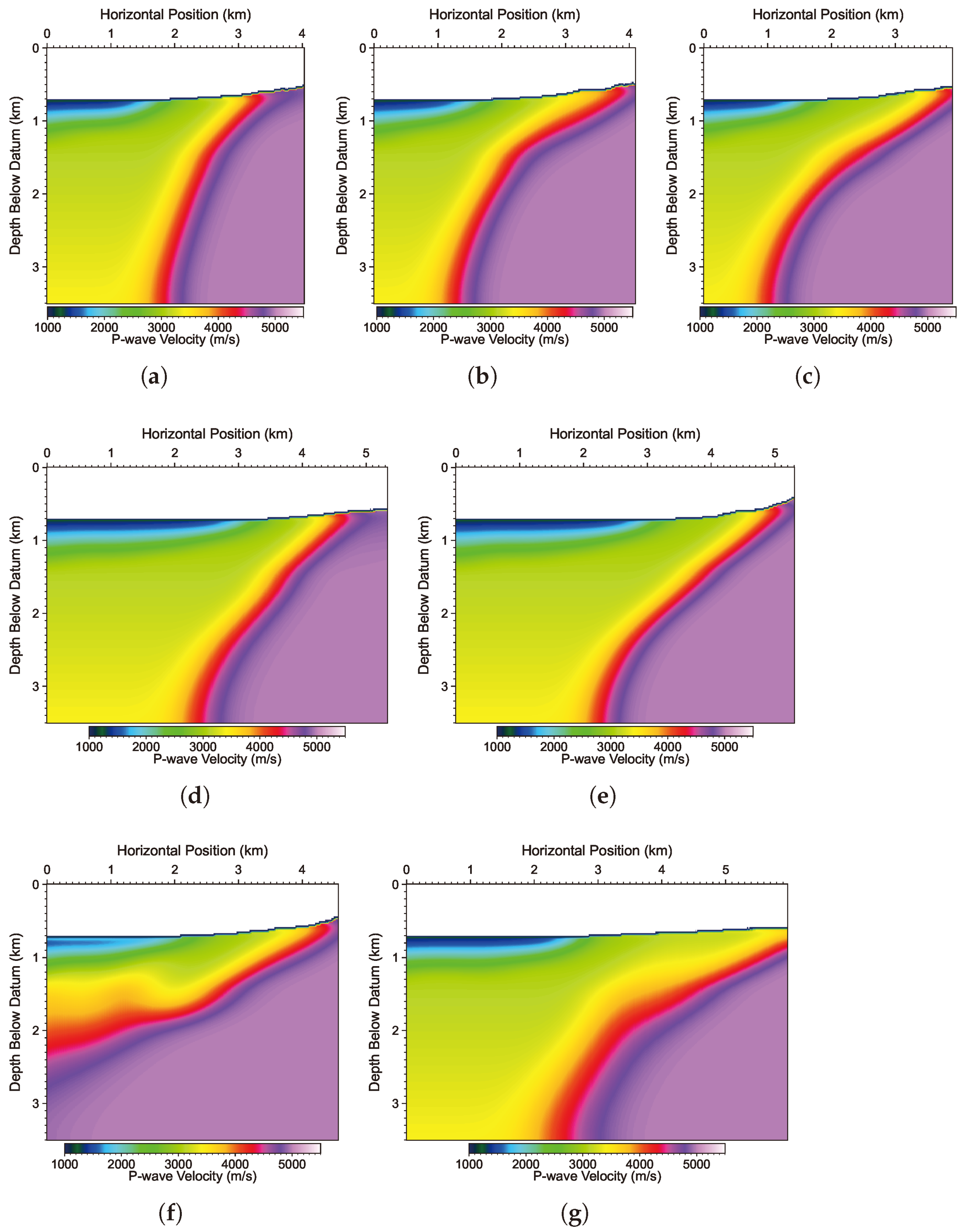The resulting initial $V_p$ model displayed in Figure 5 (the second top panel in the center column) is a smooth velocity model with similar overall geological structures consistent with the MT resistivity model. Figure 9 displays the $V_p$ models associated with the seven seismic lines. Note that the topography of this model is interpolated from the digital elevation model (DEM) with a resolution of 10 m by 10 m for this region. The DEM model is available in the United States Geological Survey (USGS) database.

3. First-Arrival Traveltime Tomography

In FATT, we obtain a refined $V_p$ model based on

$${\mathbf{m}}^{*}=\underset{\mathbf{m}}{arg\; min}\left\{\frac{1}{2}\left|\right|T_{\mathrm{syn}}-T_{\mathrm{obs}}{\left|\right|}_2^2\right\},$$

(1)

where $\mathbf{m}$ is the model parameter, $T_{\mathrm{obs}}$ is the observed traveltime, and $T_{\mathrm{syn}}$ is the synthetic traveltime. We adopt the adjoint-state FATT method [15,16] to update the initial $V_p$ model in Figure 9. We solve the forward problem in adjoint-state FATT with a second-order fast marching scheme based on the factorized eikonal equation [55,56], and the adjoint-state equation using a first-order fast sweeping algorithm [16]. We use nonlinear conjugate gradient inversion (e.g., [57]) to update the velocity model, with an optimal step size computed based on a small-perturbation strategy [58]. We use a quasi-ray-density preconditioner [59] to mitigate the energy imbalance issue associated with adjoint-state FATT. Note that we assume isotropic medium rather than anisotropic medium in the FATT, and the inversion result is a refined $V_p$ model. Anisotropic parameter models are built using full-waveform inversion detailed in the next section.

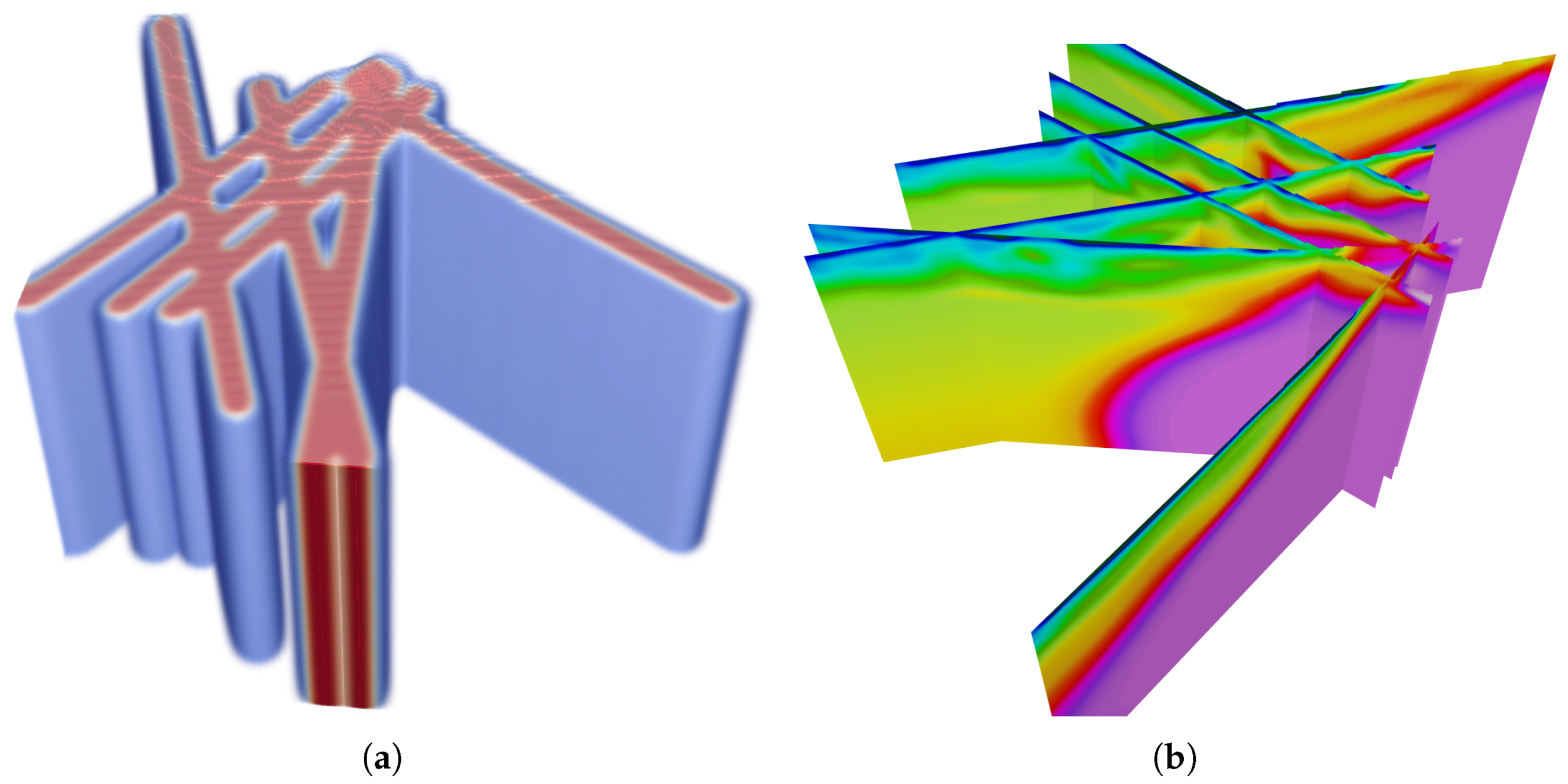
We perform one 3D FATT instead of seven 2D FATTs for the seven lines of Blue Mountain seismic data. We first create a “fat-line” mask by extending each line in their respective perpendicular directions on the horizontal plane. We then extend the mask in the depth direction to create a 3D line mask as displayed in Figure 10a. The mask value near the original position of the lines is 1, and gradually reduces to 0 away from the line. At each FATT, we multiply the computed gradient with this line mask, so that only the masked region is updated. Eventually, we obtain an updated $V_p$ model inside the mask as shown in Figure 10b. The advantage of such an FATT strategy over 2D FATT for seven separate lines is that the updated model is naturally consistent at all line intersections although the source and receivers are distributed along seven 2D lines. In addition, applying such a mask will prevent the update of the velocity model in regions that are far from the lines #x2014;such an undesirable update can happen because we use a preconditioning strategy that normalizes gradients based on approximate ray density in the inversion as describe above.

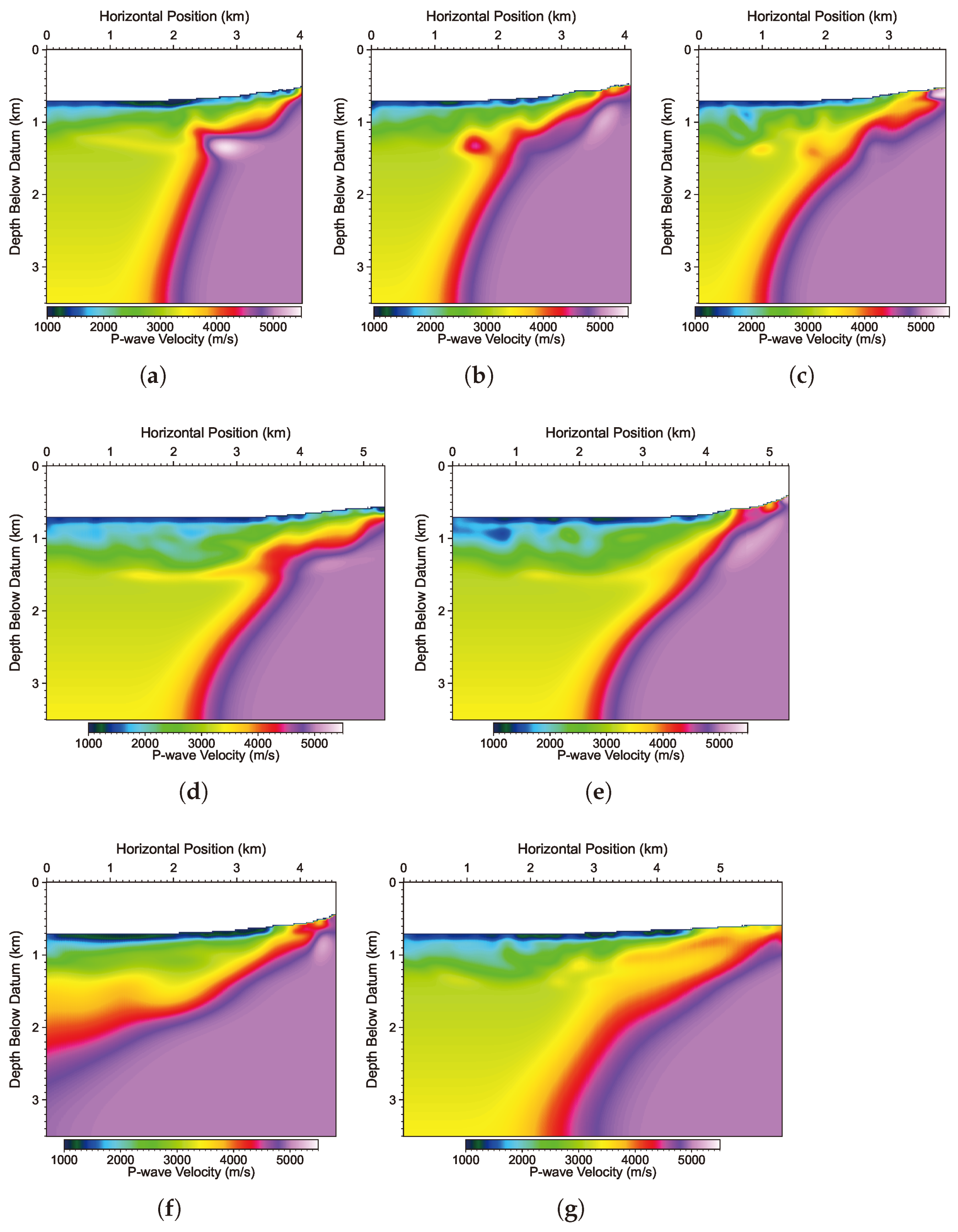
Figure 11 shows the updated $V_p$ models of the seven lines extracted from the 3D $V_p$ model in Figure 10. The maximum depth of velocity updates is approximately 1 km. Below the topographic surface, there exists a thin low-velocity layer with a velocity value around 1000 m/s and with an average thickness of approximately 100 m. The velocity and thickness of this layer is visually consistent in all seven lines. This low-velocity layer possibly consists of weathered and unconsolidated soils and degraded rocks. Below this layer, FATT produces different $V_p$ updates along different lines. The results indicate that the geology may be more complex than simple horizontal layering below the Desert Valley to the west of Blue Mountain.

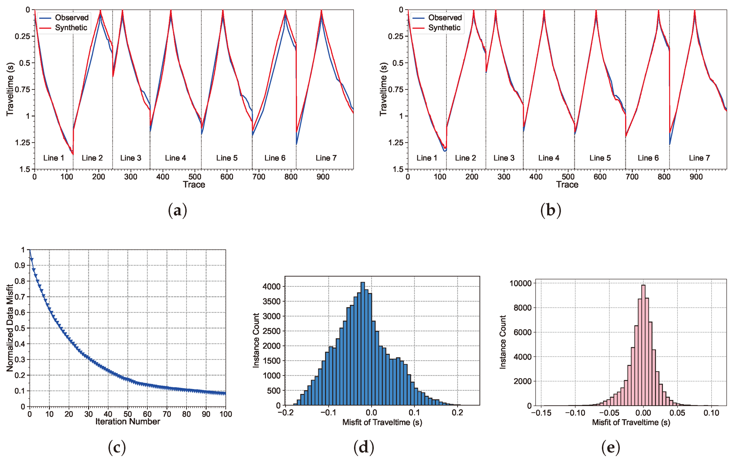
Our FATT provides a more accurate shallow $V_p$ model compared with the initial $V_p$ shown in Figure 9 in terms of traveltime fit. Figure 12a and Figure 12b compare synthetic and picked traveltime in the initial $V_p$ and in the FATT-updated $V_p$, respectively. While the initial $V_p$ model seems reasonably correct, the FATT-updated model provides an evidently better first-arrival time match. In fact, Figure 12c shows the normalized data misfit convergence associated with the FATT for these data, which indicate a 90% error reduction after 100 iterations of FATT. Further, we show the statistics of traveltime misfit in the initial and the updated models in Figure 12d,e. The misfit in the initial model can be as large as 0.2 s, along with many traces with an error between ±0.1–0.2 s and a notable shift of mean (−0.03 s). By contrast, the FATT model provides a more concentrated error distribution around zero mean, most of which are below ±0.05 s.

Our FATT result is more accurate than the initial $V_p$ model in terms of traveltime misfit error. However, because of the limited resolution and penetration depth of FATT and the sparse coverage of this seismic survey in the 3D space, it is difficult to determine the accuracy of the inverted model in terms of realistic geology of this area, particularly in a 3D sense. This is a motivation for us to perform EFWI to improve the accuracy of the FATT-updated model and perform ERTM to determine the position of reflectors.

4. Elastic Full-Waveform Inversion

In general, the maximum depth that FATT can reconstruct depends on both the available source-receiver distribution and the near-surface velocity structures. For the Blue Mountain geothermal field, we find that the maximum depth that FATT can update is approximately 1 km below the ground surface using the initial $V_p$ model in Figure 9. To obtain high-resolution elastic parameter models, we employ EFWI to update P- and S-wave velocities and anisotropic parameters up to 3.5 km below the chosen elevation datum.

We adopt the graph-space optimal-transport (GSOT) misfit function to perform EFWI [23,28]:

$${\mathbf{m}}^{*}=\underset{\mathbf{m}}{arg\; min}\left\{\sum _{i=1}^K{\left|t_i-t_{{\sigma }^{*}\left(i\right)}\right|}^p+{\left|\eta \left(d_{\mathrm{syn},i}-d_{\mathrm{obs},{\sigma }^{*}\left(i\right)}\right)\right|}^p\right\},$$

(2)

where $\mathbf{m}$ is the model parameter, t represents the time of a sample of the waveform in a seismic trace, $d_{\mathrm{obs}}$ is the observed waveform, $d_{\mathrm{syn}}$ is the synthetic waveform; ${\sigma }^{*}\left(i\right)$ is an optimal permutation solution to the linear assignment problem of GSOT by discretizing the waveforms into 2D point clouds, with the point index $i=1,\cdots ,K$ and K is the maximum number of the cloud points. We implement an auction algorithm [28] to solve the linear assignment problem. We choose $p=2$ in our GSOT implementation for simplicity. Because the computational complexity of solving ${\sigma }^{*}\left(i\right)$ is $\mathcal{O}\left(K^3\right)$ for large K, and the memory requirement is $\mathcal{O}\left(K^2\right)$, we choose a relatively small $K=500$ in our implementation. For Blue Mountain seismic data with a frequency band of 5 to 25 Hz, $K=500$ for 4-s data is sufficient; after computing the adjoint source using Equation (91) of [28], we resample K points to the original trace length using a cubic interpolator for solving the adjoint-state equation and gradient computation. In the above definition, $\eta =\tau /A$ is a scaling parameter related to the maximum time shift $\tau$ and the maximum amplitude difference A between the observed and the synthetic waveforms [28]. We choose $\tau =0.5$ s for EFWI along all seven lines. This value should be sufficient to cover the maximum traveltime difference during the inversion. By this choice, our EFWI avoids focusing on updating high-wavenumber perturbations to match amplitude, and can exploit the power of GSOT to update low-wavenumber perturbations that are essential to reveal large-scale fault structures. The Blue Mountain seismic data contain only the z-component of particle velocity field ($v_z$). Therefore, $d=d({\mathbf{x}}_r,t)=v_z\left(t\right)\delta (\mathbf{x}-{\mathbf{x}}_r)$ with ${\mathbf{x}}_r$ being the receiver locations.

We implement the EFWI using the first-order stress-velocity elastic wave Equation [60] discretized with a 16th-order standard staggered-grid finite-difference scheme and a multi-axial complex-frequency-shifted perfectly-matched layers boundary condition in the auxiliary differential equation form [61]. For source and receivers that are not aligned with regular grid points, we adopt the Kaiser-windowed sinc-function interpolation method to assign the exact source/receiver locations [62].

Fracture zones and fault zones can behave as anisotropic media for seismic-wave propagation. Accounting for subsurface anisotropic properties at the Blue Mountain geothermal field is important for reliable seismic characterization. We invert for the anisotropy up to vertically transverse isotropy (VTI) and horizontally transverse isotropy (HTI), parameterized by P- and S-wave velocities ($V_p$ and $V_s$) and two Thomsen parameters $\epsilon$ and $\delta$. In the anisotropic EFWI, we allow negative $\epsilon$, meaning that the horizontal $V_p$ is slower than the vertical $V_p$, mimicking an anisotropic medium formed by vertically or quasi-vertically aligned fractures with quasi-horizontal fracture normals and with less pressure in the horizontal direction [63]. Meanwhile, $\epsilon >0$ indicates a faster horizontal $V_p$, caused either by sedimentary layering or quasi-horizontal aligned fractures with quasi-vertical fracture normals. We do not invert for the tilt angles of tilted transversely isotropic (TTI) media in this study, because the available seismic data were collected only along sparse 2D lines that are not parallel with or perpendicular to one another. Such a configuration of data acquisition makes inversion of azimuthal rotation angles impossible. In addition, it can be difficult to directly invert for a consistent polar rotation angle for TTI without sophisticated strategies [64], given the poor quality of the Blue Mountain seismic data. Therefore, for practical considerations and for the purpose of reducing parameter trade-offs, we assume that the fractures are either VTI or HTI, where $\epsilon >0$ indicates VTI anisotropy and $\epsilon <0$ indicates HTI. Such a parameterization may not be perfect, but should be sufficient to inform the anisotropy caused by intensive fracturing in our study region as demonstrated by our results below.

We first compute the gradients associated with the elasticity parameters $C_{ij}$ and $\rho$ as described by [34] based on the adjoint sources computed using the GSOT misfit function in Equation (2). We adopt the nonlinear conjugate gradient (CG) [57] framework and the perturbation-based optimal step length computation strategy [58]. We build $V_s$ models along all seven lines by simply scaling $V_s=V_p/\sqrt{3}$, and use Gardner’s rule $\rho =310V_p^{0.25}$ kg/m ${}^3$ to build the density models. Note that the scaling factor, $\sqrt{3}$, is only for building the initial $V_s$ model; in the EFWI updates, we do not constrain $V_s=V_p/\sqrt{3}$. We simultaneously update $(V_p,V_s,\rho )$ in isotropic EFWI, and simultaneously update $(V_p,V_s,\epsilon ,\delta ,\rho )$ in anisotropic EFWI until the maximum number of iterations reaches. The gradients associated with these parameters are converted from $C_{ij}$ gradients based on the chain rule using the relationships between $(V_p,V_s,\epsilon ,\delta ,\rho )$ and $(C_{ij},\rho )$.

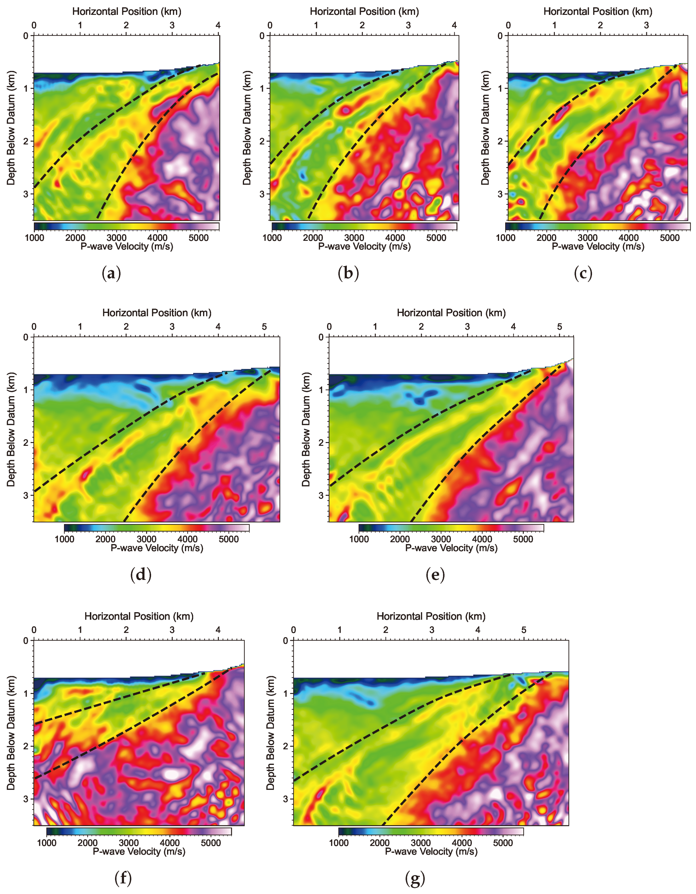
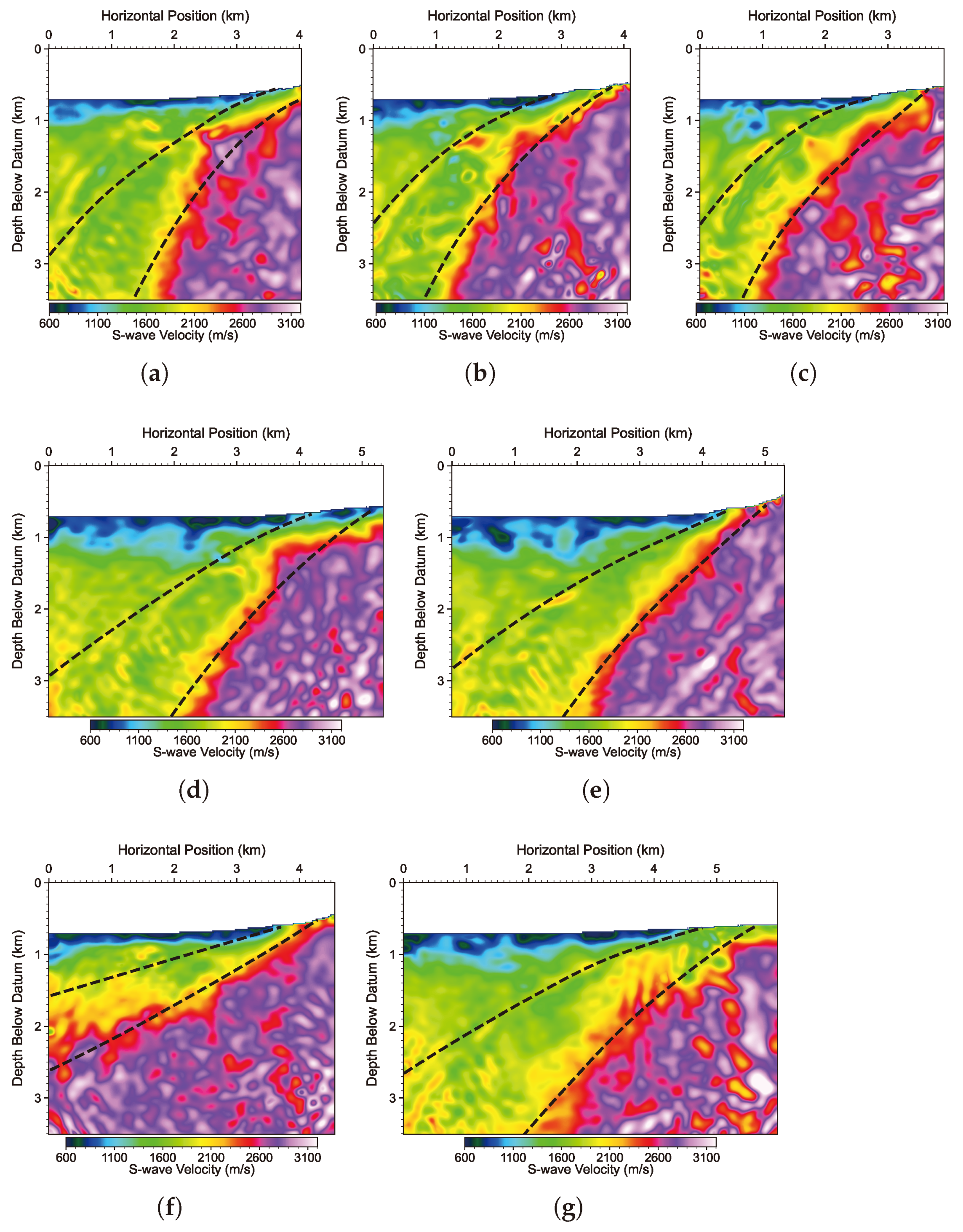
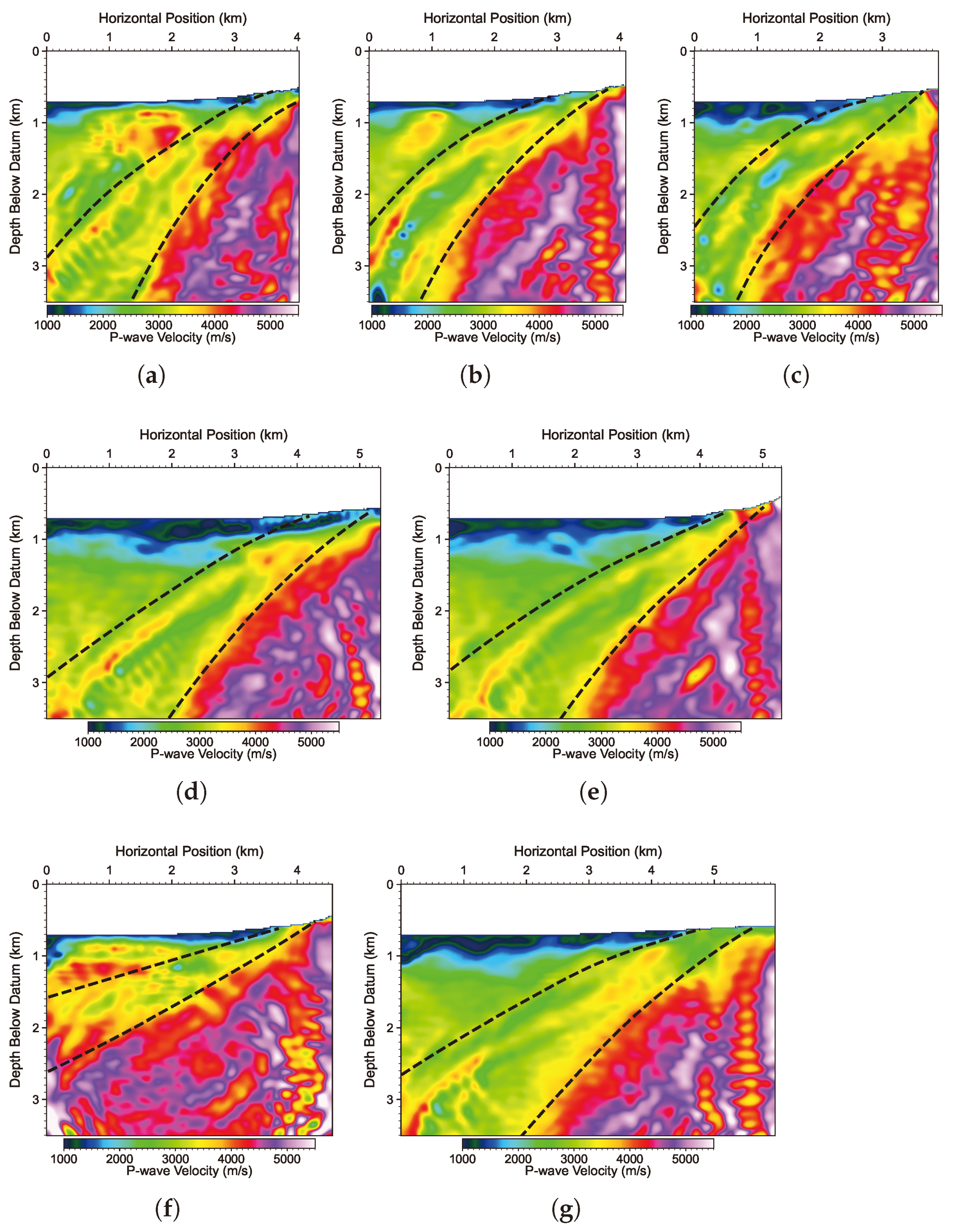
Figure 13 displays our isotropic EFWI results of P-wave velocity models for Lines 1–7, manifesting higher-resolution details than the FATT models displayed in Figure 11 in both shallow and deep regions of the models. One feature that is common to all the seven models is a low-velocity, fault-like anomaly tilting left (or west in the 3D space). We draw two curves for each model to roughly annotate the top and bottom interfaces of this feature using black dashed lines in Figure 13. 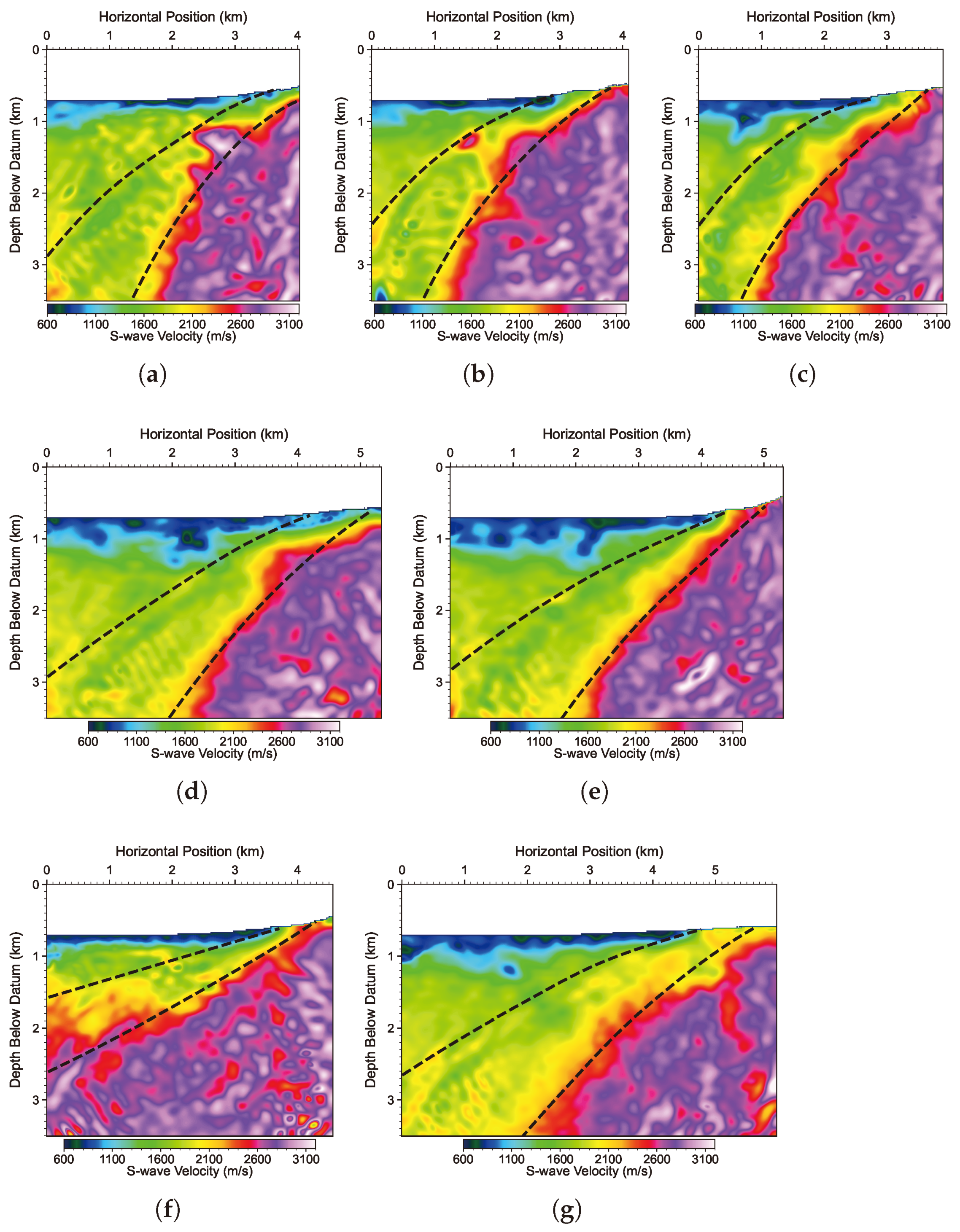This feature is not revealed in the FATT models displayed in Figure 11. Mapping this fault-zone interpretation to the updated $V_s$ models displayed in Figure 14, we find similar low-velocity anomalies. This consistency means that this low-velocity zone could be a geologically plausible feature associated with the major fault (and the resulting fault zone) in this region. In fact, the position and tilt angle of this fault zone is consistent with the large-scale geology study [1,4,5] for the Blue Mountain geothermal field, and can possibly be the NE to NNE major strike fault concealed beneath the ground surface at the west flank of Blue Mountain.

Along all the seven lines, the velocities near the ground surface are generally low (around 1000 m/s for $V_p$ and around 600 m/s for $V_s$), which should correspond to the low-velocity Quaternary sediments. Meanwhile, the velocities on the east (right) side of the lines are generally high, which may correspond to the Triassic metasedimentary rocks in this area. However, the velocity updates produced by the EFWI in the mountain region are not well constrained and exhibit some level of random fluctuations. Because of the dip angle of the major fault, the region below the mountain region, particularly at the east ends of the seven lines, may not be well covered and thus cannot be sufficiently updated compared with those in the central region of the lines. For instance, the updated $V_p$ models of Lines 2 and 6 displayed in Figure 13b,f contain some high-wavenumber heterogeneities at their lower-right corners. Since there are no well logging data at this depth and at this location, it is very difficult to quantitatively estimate how reliable these high-wavenumber heterogeneities can be.

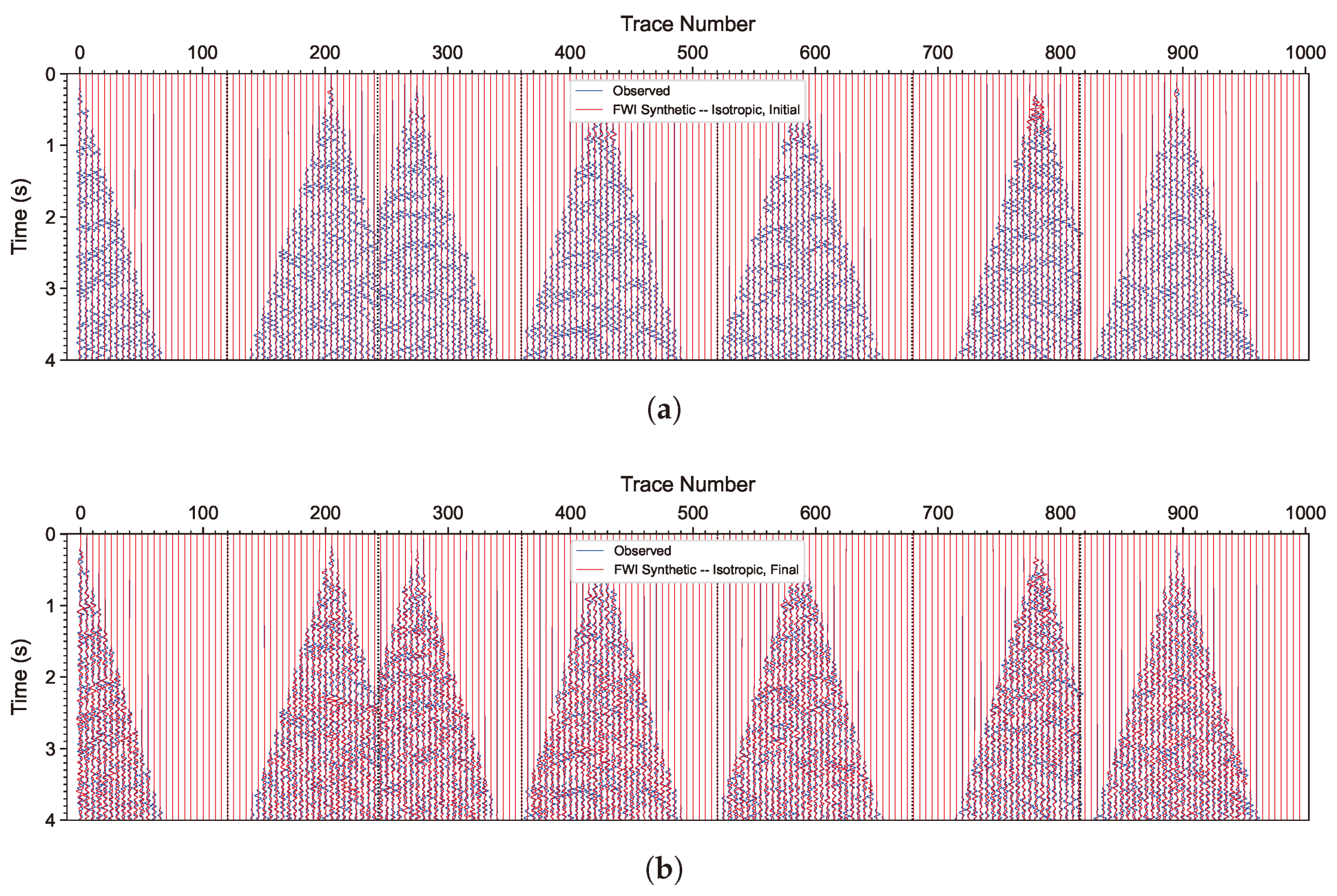
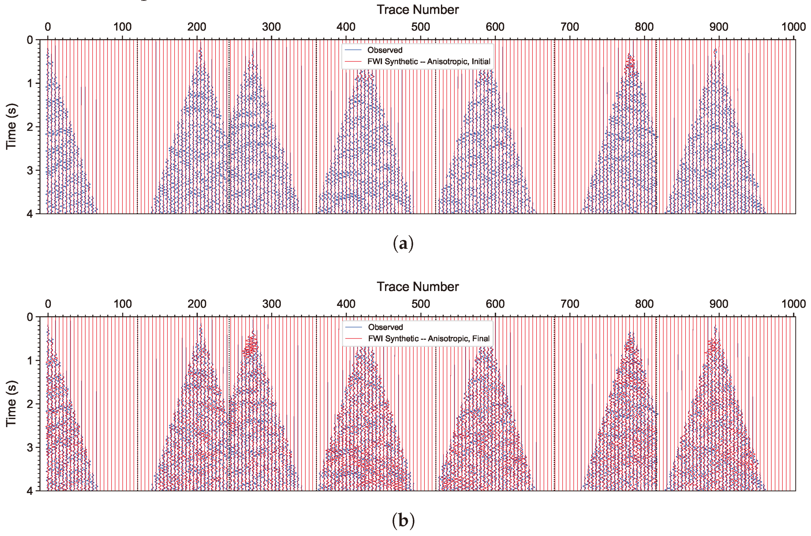
We display the waveform match of seven common-shot gathers randomly selected from the seven lines in Figure 15. Figure 15a displays the match between the observed waveforms and the synthetic waveforms generated using the initial model (i.e., the FATT-updated $V_p$ and converted $V_s$ and $\rho$ based on this $V_p$). Both data are displayed in their original amplitude without any scaling. The initial model is too smooth to generate any visible reflections, so the red wiggles are almost flat with zero amplitude. By contrast, Figure 15b displays the match between the observed waveforms and the synthetic waveforms generated using the EFWI-updated models displayed in Figure 13 and Figure 14. Even though the waveform match is still not very good, we find that major reflection events are well matched both in amplitude and arrival time, manifesting a major improvement over that in Figure 15a. In fact, the normalized data misfits associated with the isotropic EFWI for the seven lines reduce to approximately 30% to 40% as shown by Blue curves in Figure 16.

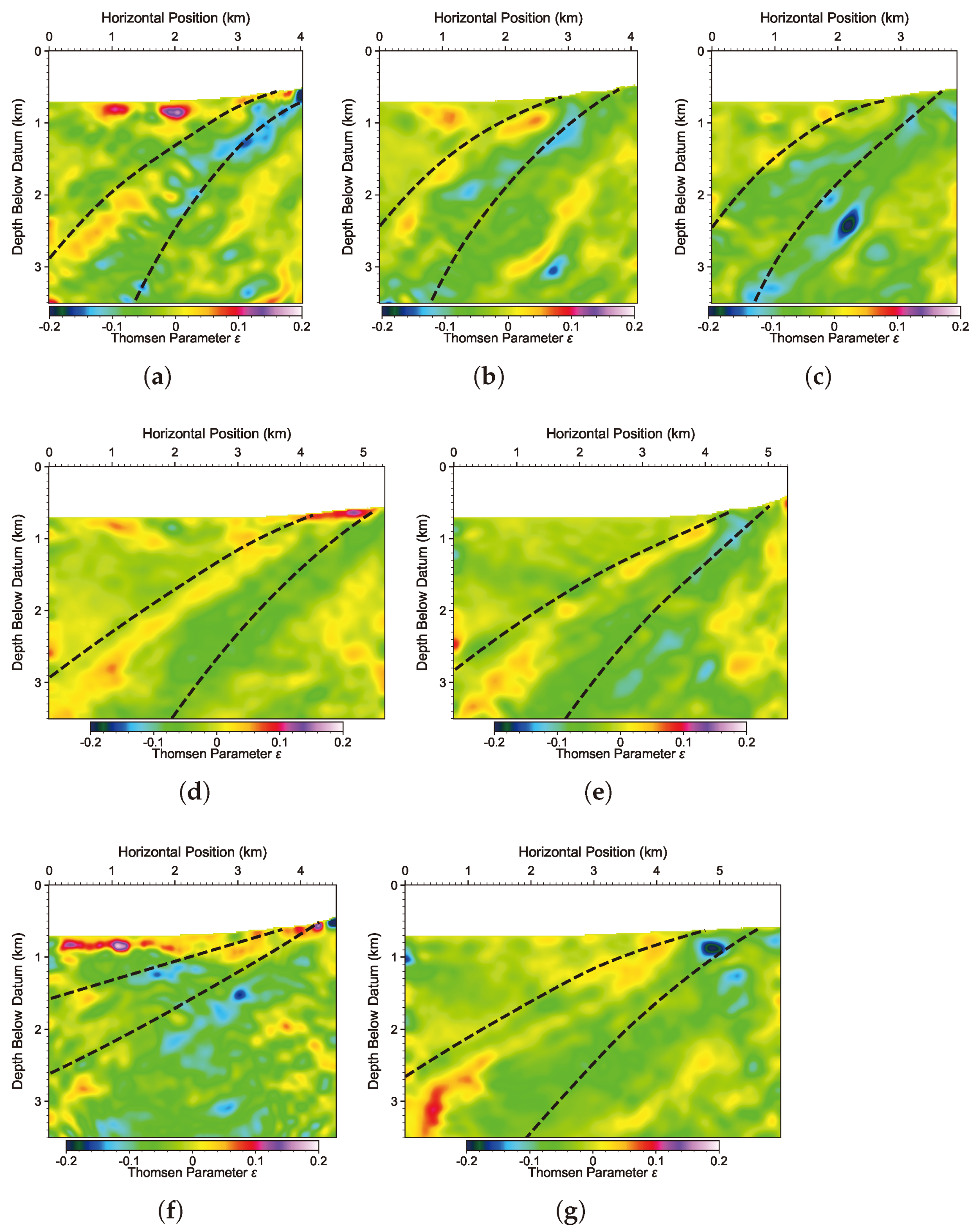
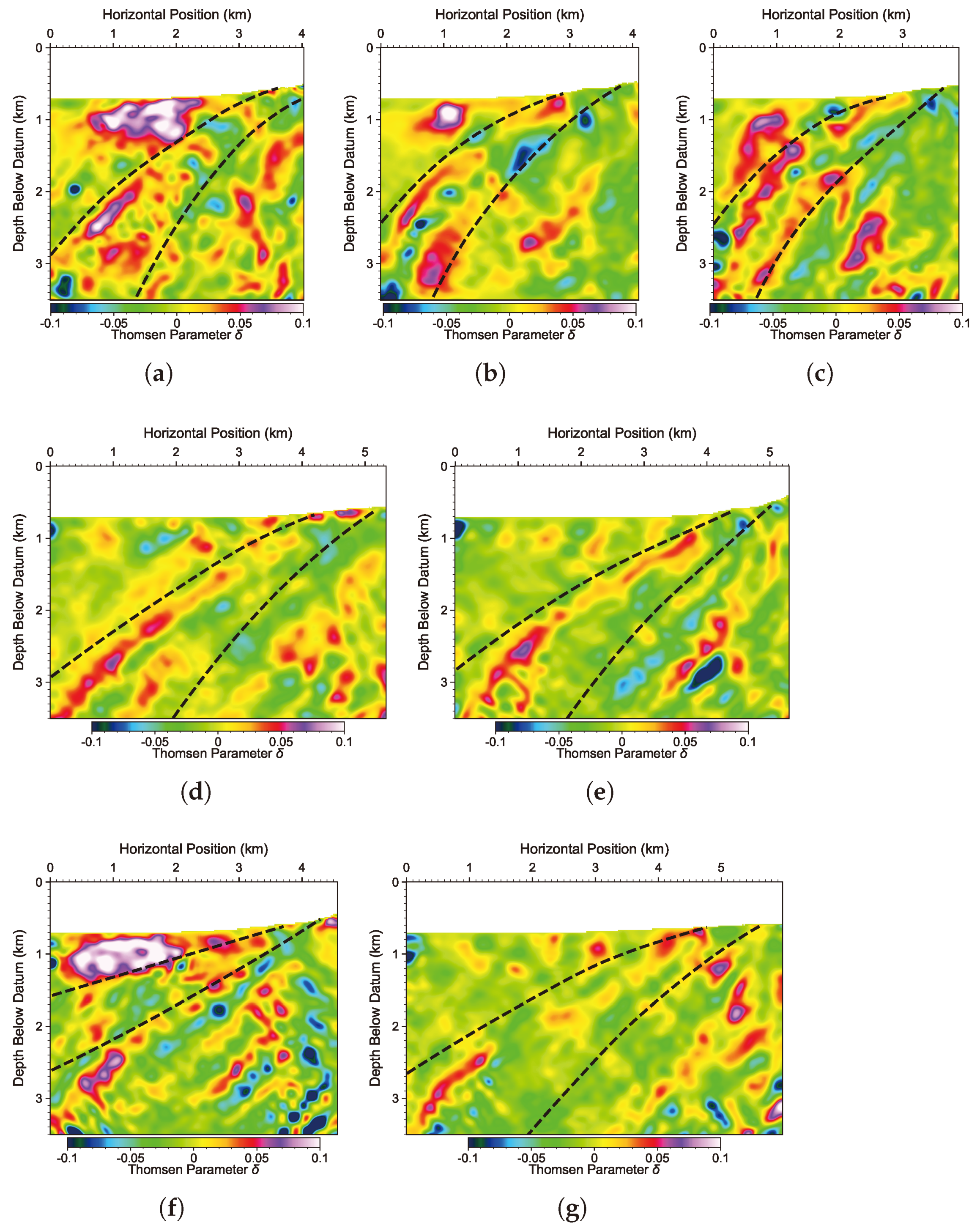
We further perform anisotropic EFWI using the same data and the same initial models ($V_p$, $V_s$ and $\rho$). The starting models of $\epsilon$ and $\delta$ are zero, and we allow both parameters positive or negative as aforestated. Figure 17, Figure 18, Figure 19 and Figure 20 show the inverted $V_p$, $V_s$, $\epsilon$, and $\delta$, respectively. Visually, the $V_p$ and $V_s$ models display no significant differences from their isotropic EFWI counterparts in Figure 13 and Figure 14. The only difference shown in the anisotropic EFWI $V_p$ and $V_s$ models is that the low-velocity anomalies within the annotated fault zone seem to be more consistent in depth and more interpretable than those obtained using isotropic EFWI. For instance, we observe a tilt layer of high-velocity anomaly in isotropic $V_p$ models of Lines 2 and 3 displayed in Figure 13b,c. This high-velocity structure can be difficult to interpret for a major fault zone where intensive fracturing and thus low-velocity structures should dominate. In the $V_p$ models inverted using anisotropic EFWI, as displayed in Figure 17b,c, we observe much weaker or no high-velocity structures, leading to a more reasonable interpretation of the inversion results and an improved structure consistency with the inverted $V_s$ models in Figure 18.

We find that the hand-picked fault lines (black dashed lines) correlate reasonably well with the large structures of the updated $V_s$ models in Figure 18. We map these fault annotations to the updated $\epsilon$ models in Figure 19, and find that they are generally in good spatial correlation with the negative anomalies of $\epsilon$, particularly beneath Lines 1 to 5. As mentioned earlier this section, negative $\epsilon$ in our EFWI indicates the vertical velocity is faster than the horizontal velocity and thus HTI anisotropy. Such velocity anisotropy is possibly caused by the intensive fracturing and faulting in this major fault zone, and indicates higher fracture density in these regions. The $\delta$ parameter is more difficult to interpret as it involves both normal and shear elasticity. In fact, the delta inverted here is usually referred to as a “garbage collector” to correct for reflectivity mismatch, and therefore, as we expect, it has evident high-wavenumber variations like a migration result. This is explained in detail in [65,66]. Nevertheless, when mapping the fault-zone boundary lines to the inverted $\delta$ models as displayed in Figure 20, we find that there are some spatial correlations, although weak, between the pattern of $\delta$ heterogeneity and the annotated fault-zone boundary lines, particularly at Lines 1 to 5.

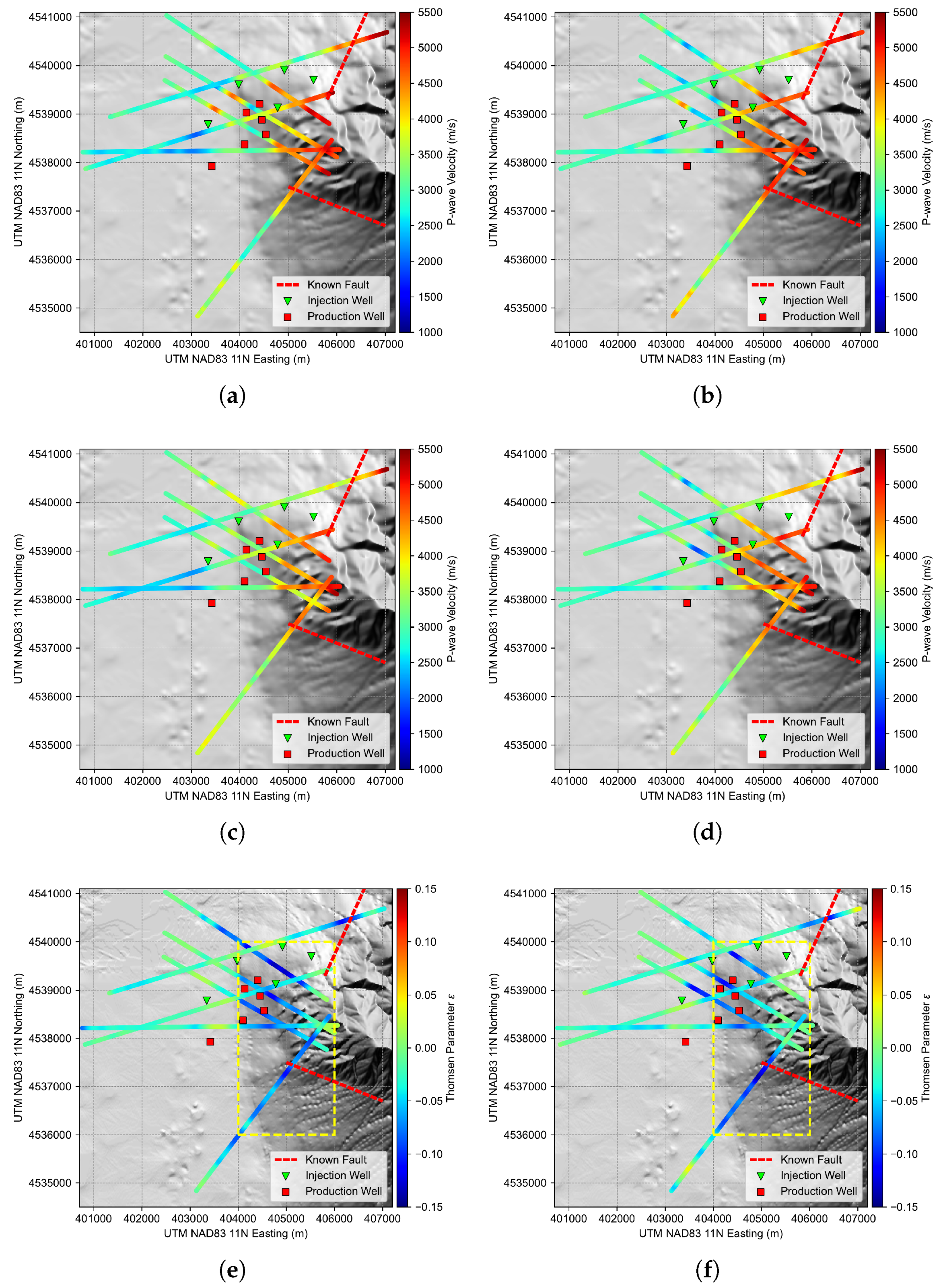
The additional structural constraints provided by the anisotropic EFWI become more evident when we map our isotropic EFWI and anisotropic EFWI results on the map view. Figure 21a,b display the depth slices of 1400 m and 1600 m of the updated $V_p$ models in Figure 13, along with the spatial locations of injection and production wells. The depth at 1600 m corresponds to the bottom of current production wells. At both depths, we find that the inverted $V_p$ exhibits both high and low anomalies along the extension of lines. We are unable to interpret a meaningful spatial trend of the velocity anomalies. By comparison, Figure 21c,d display the depth slices of $V_p$ produced by anisotropic EFWI. There are less inline velocity fluctuations and the values at line intersections are more consistent. High and low velocities exhibit a relatively more evident boundary on the west flank of Blue Mountain, and all the production wells sit on the mid- to low-velocity region at these two depths. Figure 21e,f display the inverted $\epsilon$ at the two depths. In these two plots, blue colors represent negative $\epsilon$ (faster vertical velocity), and thus possibly high fracture density. Six of the seven lines exhibit strong spatial correlation in negative $\epsilon$ on the west flank of Blue Mountain, enclosing almost all the injection and production wells in this geothermal field. The consistent pattern indicates a highly possible fracture zone covering 4 km in the NS direction (4,536,000 to 4,540,000 m) and 2 km in the WE direction (404,000 to 406,000 m) annotated as the yellow dashed rectangles in Figure 21e,f. The position of this region is consistent with that determined by the large-scale geology and regional fault model, e.g., Figure 6 of [1], Figure 2 of [5], Figure 3 of [2], and Figure 1 of [3]. Note that there is only surface location of the faults available in these previously published results. Based on the physical meaning of $\epsilon$ [63], we can conclude that in the line-intersection zone where the production and injection wells are placed, the fractures are approximately perpendicular to Lines 1–3. The concentration of negative $\epsilon$ to the southwest of Blue Mountain (i.e., on Line 6) is consistent with the known fault that trends SE-NW on the south flank of Blue Mountain; the value of $\epsilon$ also indicates that the fracturing might be perpendicular to Line 6 on the southwest flank of Blue Mountain. In addition, we notice a negative $\epsilon$ zone at the east end of Line 7. According to the fault mapping by [2,5], this feature is possibly correlated with the NE-trending major fault that controls the deformation of this region.

For the anisotropic EFWIs, we obtain data misfit convergence (displayed in Figure 16 red curves) and waveform match (displayed in Figure 22) that are similar to those of the isotropic EFWIs. Only at some lines (Lines 3 and 6), the inversions converge to slightly lower misfit. Therefore, in terms of data misfit and waveform match, we do not find significant improvement provided by anisotropic EFWI. Considering the signal-to-noise ratio of these data, the convergence comparison indicates that even with more degrees of freedom to fit the data, high-fidelity EFWI could be challenging for land seismic data. In such a situation, more sophisticated strategies or methods may be required to further improve the waveform match, e.g., using multi-component elastic-wave data, or introducing even more anisotropy or attenuation parameters.

5. Elastic Reverse-Time Migration and Fault Detection

We adopt a hybrid-domain ERTM method to obtain the PP and PS images in both isotropic and anisotropic models [61]:

$$I_{AB}\left(\mathbf{x}\right)=\Re \left\{{\int }_{{\omega }_{min}}^{{\omega }_{max}}\left\{{\mathbf{A}}_s·{\mathbf{B}}_r^{*}-{\mathcal{H}}_z\left[{\mathbf{A}}_s\right]·{\mathcal{H}}_z\left[{\mathbf{B}}_r^{*}\right]-{\mathbf{A}}_s·{\mathcal{H}}_z\left[{\mathbf{C}}_r^{*}\right]-{\mathcal{H}}_z\left[{\mathbf{A}}_s\right]·{\mathbf{C}}_r^{*}\right\}d\omega \right\},$$

(3)

where the subscripts A and B indicate P or S-wave component, ${\mathbf{A}}_s$ and ${\mathbf{B}}_r$ are the frequency-domain representation of the source and receiver wavefields of the A and B components, and ‘${}^{*}$’ represents complex conjugate. The wavefield ${\mathbf{C}}_r$ is computed from an auxiliary back-propagated wavefield with the temporal Hilbert transform of recorded seismic data as the source term at the receiver locations. ${\mathcal{H}}_z$ represents the Hilbert transform in z-direction. We perform low-rank decomposition to obtain the vector P- and S-wavefield components to ensure consistent S-wave polarity [42,61].

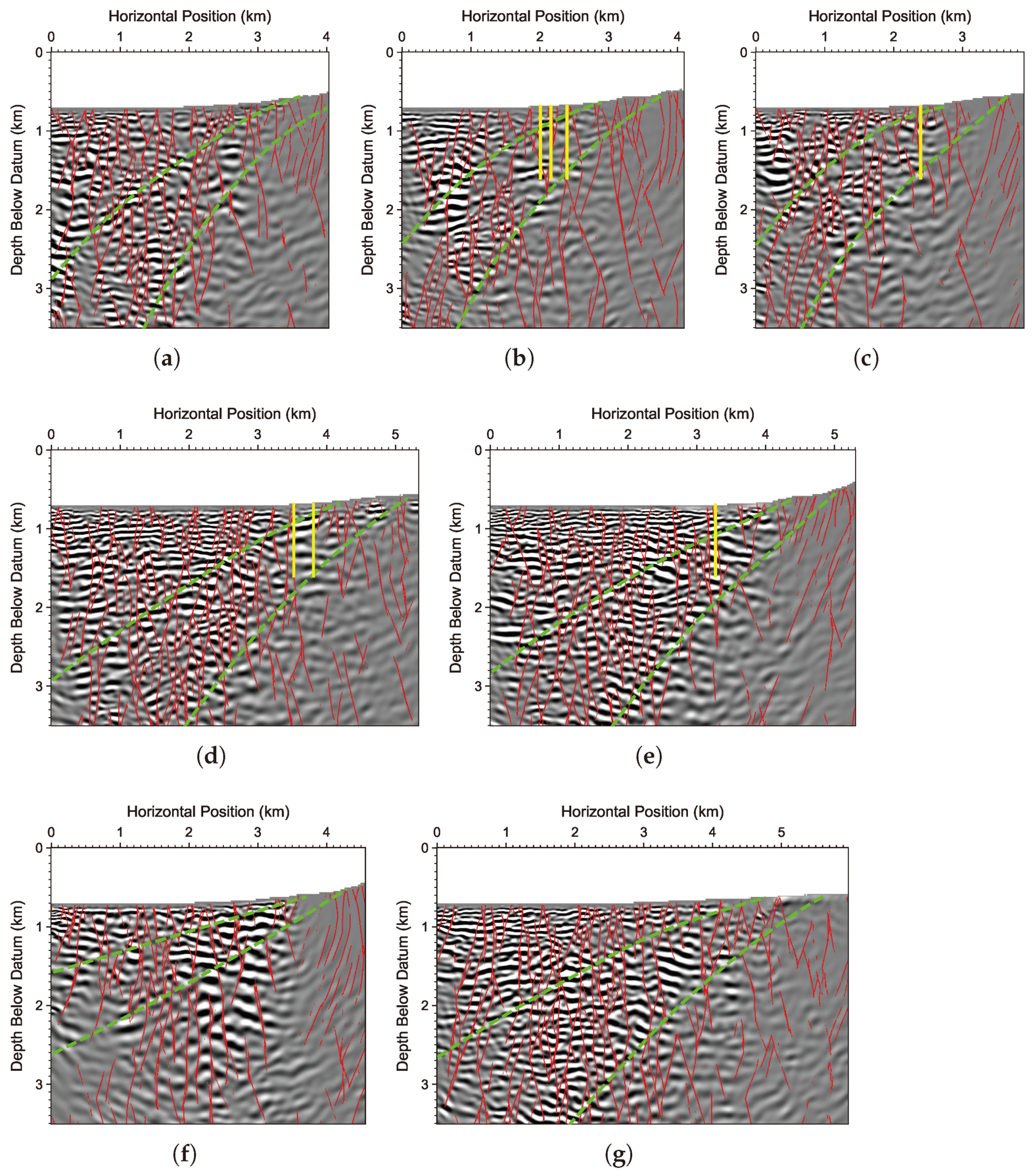
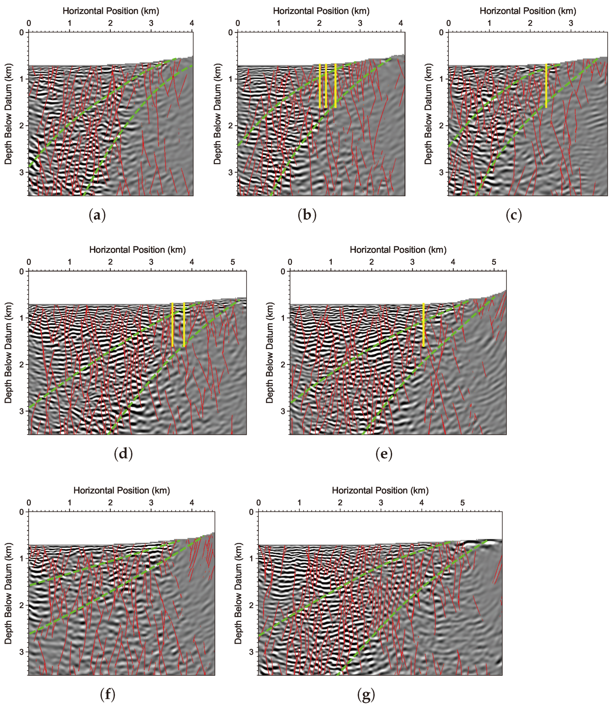
With the imaging condition (3), we produce PP and PS images using the updated elastic parameters obtained using isotropic and anisotropic EFWI. Figure 23 and Figure 24 display the PP and PS images produced using our isotropic EFWI models in Figure 13 and Figure 14. We also overlay the faults detected on the images using our machine learning algorithm [47].

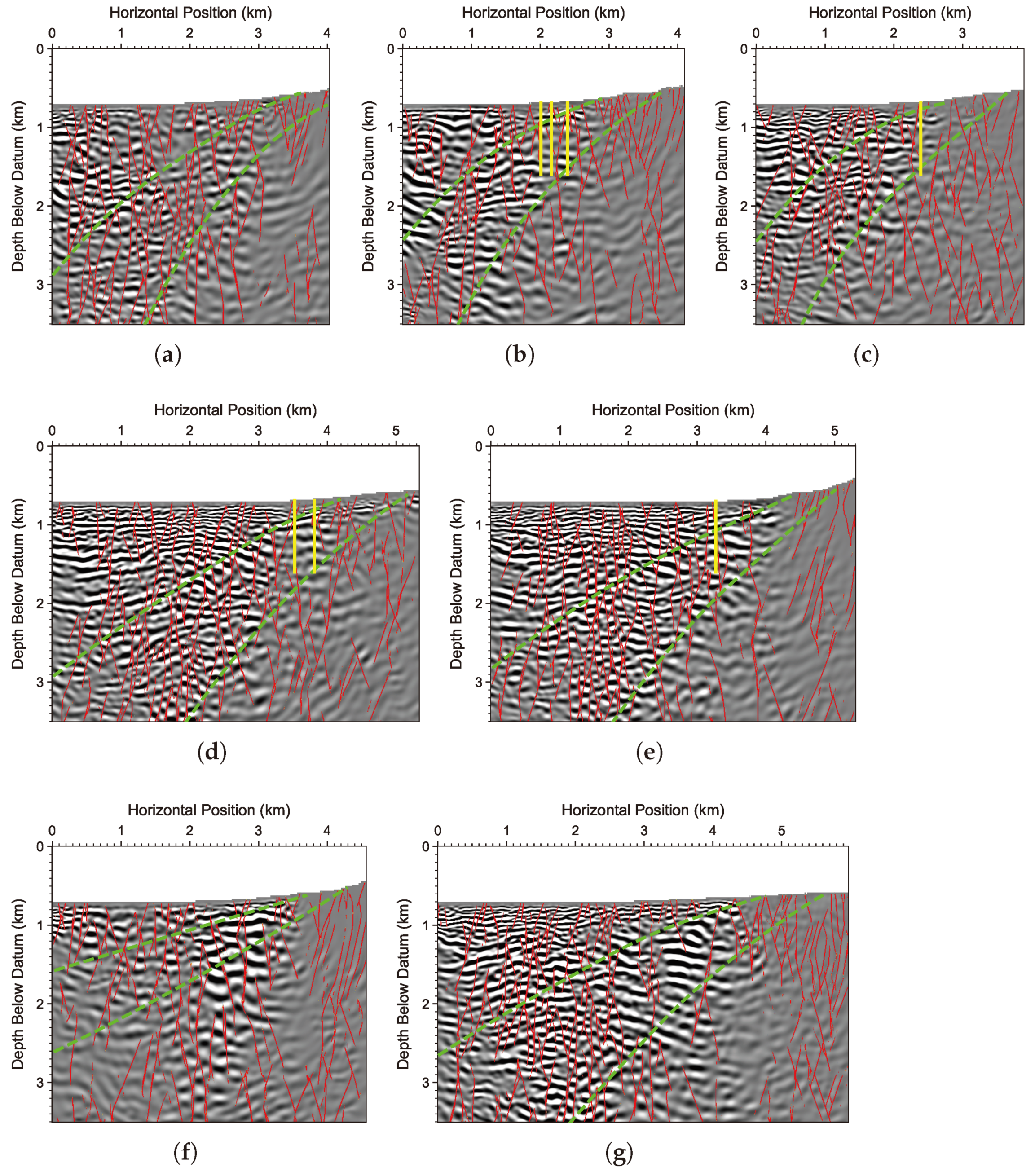
For all seven lines, the PS images show higher vertical resolution compared with the PP images, a natural characteristic of ERTM because S-waves have shorter wavelength in space. We find that both the PP and PS images for all the seven lines show numerous discontinuities along their respective seismic line direction, and it is difficult to observe continuous reflectors that span the entire seismic lines in the horizontal direction. Our ML-based fault detection interprets lateral discontinuities of reflectors as faults. This may not be completely accurate under certain circumstances (e.g., when an image has imaging artifacts caused by noise or poor illumination, and so on). Nevertheless, given this assumption, inside the possible fault zone annotated by the green dashed lines, we observe higher fracture density than that outside of the fault zone, indicating intensive faulting and fracturing may have occurred.

Existing fault maps and conceptual geological models for this region built based on geological modeling and drilling [2,3,5] show numerous moderately (50–60 degrees) west-dipping normal faults that host the up-flow and production of geothermal fluids. The high-angle ML-detected discontinuities may be Miocene diorite dikes and sills intruded into the Triassic meta-sediments. However, according to [3], in wells drilled on the south edge of the geothermal field, the intrusives are not found in the shallowest 900 m of the metasediments, but increase to 40–43% of the formation between 1527–2442 m in depth. Thus, there should not be a large number of faults penetrating to the shallow ground surface. Instead we prefer to interpret the ML-detected discontinuities as secondary, small-scale faults or fractures. Even in that interpretation, some of the ML-detected faulting features shown in Tertiary and Quaternary basin fill sediments above the metasediments in Figure 23 and Figure 24 are possibly a result of over-detection based on a migration image that has imaging artifacts using our ML method. The data-labels (i.e., image-fault pairs) for training our fault detection neural network mainly consist of high-angle faults that penetrate from the top to bottom of images, and as a result it may over-detect when a realistic fault stops in the middle of the image. In addition, faults with different displacements have equal probability of one in our training dataset, which leads to detected faults, either with a large or small fault displacement, having the same fault probability. In other words, if a fault on an input image to our fault detection NN only has a small displacement (like many faults in Figure 23 and Figure 24), it can still be recognized as having a probability of one using our method. Accurately estimating the fault displacement of different faults may need new ML models, which is beyond the scope of this work. At this stage, it is difficult for us to validate the accuracy of these detected faults using field experiments (e.g., well drilling). Nevertheless, the production wells at the Blue Mountain geothermal field extract geothermal energy from faults, and we project nearby geothermal production wells onto Lines 2–5 and plot them using yellow straight lines in Figure 23b–e. We find that all these production wells penetrate into the low-velocity zone (green dashed lines) with high density of ML-detected faults (red lines). This consistency may indicate the efficacy of our ERTM results and fault detection.

We also produce the PP and PS images in Figure 25 and Figure 26 using anisotropic ERTM in the anisotropic EFWI models shown in Figure 17, Figure 18, Figure 19 and Figure 20. We again render our ML-detected faults on these images. The images exhibit similar discontinuity characteristics to their isotropic counterparts in Figure 23 and Figure 24. For Lines 1–3 and 6, high fracture density and mostly high dips of these fractures seem to be in good correlation with the negative $\epsilon$ values in this fault zone displayed in Figure 21e,f. A minor difference between the isotropic and anisotropic ERTM PP images of Line 7 (shown in Figure 23g and Figure 25g, respectively) is that the east end of anisotropic EREM PP image contains more detected faults than the isotropic ERTM PP image. This is consistent with the low $\epsilon$ value at the end of Line 7 as shown in Figure 21e,f. This feature is possibly caused by the NE-trending major strike fault in this region. More recent fault imaging and fracture characterization methods, such as angle-controlled ERTM [67] and double-beam neural network [68], may further help delineate faults and detect/characterize fracture zones at the Blue Mountain geothermal field.

6. Discussion

In the EFWI section, we demonstrate the effectiveness of our EFWI strategy to reveal high-resolution subsurface structures at the Blue Mountain geothermal field. In particular, we use the inverted $V_p$ model generated by 3D line-masked FATT as the initial model for EFWI. The 3D line-masked FATT model is naturally consistent at every line intersection point. However, because we perform 2D EFWI instead of 3D line-masked EFWI as in FATT, it is intriguing to check whether the isotropic and anisotropic EFWI results can correlate well at the line intersection points.

Figure 27a,b show the $V_p$ and $V_s$ models of Lines 3 and 4 produced by isotropic EFWI, while Figure 27c,d show the $V_p$ and $V_s$ models of Lines 3 and 4 produced by anisotropic EFWI. We use black ellipses to highlight locations where anisotropic EFWI produces an evident improvement of consistency over isotropic EFWI. This comparison indicates that by using an anisotropic medium assumption, EFWI can lead to improved line intersection consistency. However, such consistency does not hold at every line intersection point considering the complex land seismic data and complex subsurface structures associated with this survey, because there are no direct spatial constraints among different lines during separate, 2D EFWI model update. If the EFWI is performed in a line-masked approach as the 3D FATT, then the resulting updated models will be naturally consistent for both isotropic and anisotropic EFWI, but at a much higher computational cost. Such trade-off should be carefully weighed before seismic characterization for similar geothermal fields.

We observe similar improvement on the migration images generated by isotropic and anisotropic ERTM as displayed and highlighted by red ellipses in Figure 28.

Even though the seismic characterization results presented in this paper demonstrate the effectiveness of our workflow, there may exist several potential shortcomings. First, our EFWI does not consider the effect of intrinsic attenuation. That is, we do not invert for quality factors during EFWI. In addition to the amplitude distortion caused by heavily weathered near-surface soils and rocks, a hydrothermal system like Blue Mountain geothermal reservoir may possess strong intrinsic attenuation caused by intensive fracturing and faulting [69]. It is well known that ignoring the attenuation effect in FWI/EFWI and RTM/ERTM may lead to notable inaccuracies. Recent studies also find that thermo-poroelasticity of heated rocks may further complicate behaviors of seismic waves that propagate through [70]. Properly including all these complex mechanisms may result in more accurate seismic characterization, but is beyond the focus of this paper. Second, in this study, we adopt the classical anisotropy parameterization based on the Thomsen parameters for EFWI. The parameterization may not be the optimal choice for the data we have. Alternative parameterization strategies [36,64,65,66] may improve the inversion results to be more geologically correlative to reality in the Blue Mountain geothermal field. Third, we do not consider TTI, because, as we state in the EFWI section, in practice it is challenging to reliably estimate the tilt angle of TTI with the available seismic data and the data acquisition geometry at the Blue Mountain geothermal field. Properly estimating TTI anisotropy for this field may require wide-azimuth, long-offset, and high-quality multi-component seismic data acquisition. Alternative forms of TTI parameterization (e.g., TI anisotropy constrained by the reflector normal as described by [71]) may also facilitate deriving more reliable anisotropic parameter models.

7. Conclusions

We performed an active-source seismic characterization of the Blue Mountain geothermal field in Nevada using active seismic data acquired along seven 2D lines. We have denoised the seismic data to obtain coherent reflections using an unsupervised machine learning method, and built a low-resolution initial $V_p$ model based on the existing MT survey result. We performed 3D line-masked first-arrival traveltime tomography using the hand-picked traveltimes, and performed 2D isotropic and anisotropic elastic full-waveform inversion and elastic reverse-time migration using the denoised data and tomography results. We have obtained a set of high-resolution elastic medium parameter models and migration images, and have used a supervised machine learning method to obtain fault maps on the migration images. The analysis of the spatial correlation between the inversion results and local geology revealed that the inversion results correlate well with known faults and production well locations in this geothermal field. Our inversion and imaging mapped complex subsurface structures at the Blue Mountain geothermal field. The results provide valuable information for siting additional wells to increase energy production at the Blue Mountain geothermal power plant.