Article

Machine Learning-Based Estimation of COP and Multi-Objective Optimization of Operation Strategy for Heat Source Considering Electricity Cost and On-Site Consumption of Renewable Energy

School of Engineering, The University of Tokyo, Tokyo 113-8656, Japan
*
Author to whom correspondence should be addressed.
Energies 2023, 16(13), 4893; https://doi.org/10.3390/en16134893
Submission received: 1 December 2022 / Revised: 30 May 2023 / Accepted: 3 June 2023 / Published: 23 June 2023
(This article belongs to the Special Issue Forecasting and Risk Management Techniques for Electricity Markets II)

Abstract

:
Air conditioning is a significant consumer of electricity in buildings, accounting for around 40% of the total consumption. While previous studies have focused on planning methods to minimize electricity costs, recent years have seen an increasing need for energy management methods that consider environmental performance, such as CO2 emissions, alongside economic efficiency. This study proposes a mechanism to support stakeholders’ decision-making by calculating Pareto solutions based on the multi-objective optimization of economic and environmental characteristics for entities that own renewable energy generation facilities. Unlike many existing studies that assume a specific equation for COP (Coefficient of Performance) estimation, this study adopts a nonparametric COP estimation method using machine learning, resulting in a more realistic and flexible modeling of the system. The study also presents a model for selecting an operation strategy that balances environmental and economic goals, incorporating a thermal storage facility to improve the renewable energy rate. Specifically, we proposed and compared methods for calculating solutions using only the GA (Genetic Algorithm) and a two-step optimization method combining a GA and gradient-based optimization method, confirming the superiority of the two-step optimization method. The case study unveiled unique operational profiles corresponding to cost-saving, renewable-energy, and balanced orientation points, suggesting the existence of specific strategies tailored to each orientation. The findings of this study can help stakeholders make more informed decisions regarding energy management in air conditioning systems, with benefits for both the environment and the bottom line.

1. Introduction

1.1. Background

Air conditioning is a critical component in buildings and consumes a significant amount of electricity, accounting for around 40% of the total energy usage. In central heat source air conditioning, heat generated by the equipment is transferred to air conditioners through pipes, where the air and heat medium exchange heat to cool or heat the air. In large-scale central heat source systems, there are multiple heat source devices, and their operation and shutdown must be scheduled according to the demand for heat. To optimize the efficiency of daily energy equipment operation, energy consumers need to consider various factors, such as fluctuations in renewable energy generation due to weather conditions, fluctuations in equipment efficiency, fluctuations in electricity prices, and the use of energy storage and thermal storage facilities. Furthermore, during the equipment installation phase, it is essential to determine the appropriate scale of the equipment to be installed. With the increasing focus on the introduction of renewable energy and the establishment of decarbonization targets, energy management methods based on multi-objective optimization have gained attention. These methods aim to address not only economic efficiency, but also environmental efficiency, such as reducing CO2 emissions and achieving other environmental goals. In this study, we propose a multi-objective optimization approach to develop a strategy for the daily operation of existing HVAC (Heating, Ventilation, and Air Conditioning) equipment. The proposed method aims to minimize power costs while maximizing on-site consumption of renewable energy. It takes into account various variable factors such as equipment efficiency and solar power generation to reflect the reality of daily operations. To verify the effectiveness of our proposed approach, we conduct a case study using actual operating data of multiple heat source equipment and thermal storage units at an airport.
Overall, our study presents a method to support stakeholders in decision-making related to energy management in the air conditioning domain. It offers a more realistic and flexible modeling of the system by using a nonparametric COP (Coefficient of Performance) estimation method based on machine learning, which is then incorporated into the optimization equation. By doing so, we can achieve a better balance between the environmental and economic performance in HVAC operations, which is crucial for promoting sustainable energy consumption.

1.2. Related Work

This section focuses on the optimization of heat source equipment, with a particular emphasis on thermal energy storage devices. These devices act as a form of energy storage and can shift the electricity demand, similar to how storage batteries function. As such, this section not only reviews studies on the optimization of heat source equipment, but also considers research on the optimization of electricity management, including storage batteries.
In the operation strategy of heat source equipment, demand shift can be achieved by using thermal energy storage (TES: Thermal Energy Storage) equipment such as ice thermal storage tanks. Existing TES systems are often operated on a fixed schedule and do not take advantage of their load shifting capability; appropriate demand shifting with TES and storage batteries can reduce costs by utilizing the price difference in time-of-use (TOU: Time Of Use) electricity rates and the surplus of renewable energy [1,2,3,4] and suppressing annual peaks in electricity demand [5,6,7].
Studies using multi-objective optimization in the field of energy storage and thermal storage include minimizing the cost of electricity and the probability of power loss through the operation of storage batteries [8,9,10], respectively; Abdelkader et al. [8], Ould Bilal et al. [9], and Yang et al. [10] have investigated the impact of stand-alone environments on energy prosumers consisting of wind-solar PV systems, storage batteries, and electricity demand. They formulated the cost of electricity and the probability of power loss, and by employing a genetic algorithm, they solved a multi-objective optimization problem aiming to minimize both. This approach facilitated the identification of facility installations that are both economically viable and robust. This optimizes parameters, such as the size of the wind power, solar power, and storage battery installations and the angle at which they are installed, and not for day-to-day operational strategies. Additionally, due to the stand-alone environment, the system’s behavior regarding a power purchase from the grid was not considered. Another multi-objective optimization study from the environmental and economic point of view of storage batteries is the multi-objective optimization [11,12], which considers CO2 emissions and power usage costs. The object being optimized here is not the charging and discharging schedule, but rather the capacity and other parameters of the facility while the heat storage and heat dissipation and the charging and discharging are rule-based and fixed. Therefore, this is not a discussion of day-to-day operational strategies. Thus, in the multi-objective optimization of energy systems, including storage batteries, which are similar to the heat source and thermal storage equipment that are the subject of this study, the scale of the system installation that achieves both environmental and economic performance through multi-objective optimization has been calculated, but the effects were obtained through a multi-objective optimization of operational strategies at a certain installation scale. However, there is still room for research on the effects that can be obtained with a multi-objective optimization of operational strategies at a certain scale of installation.
As for the optimization of the system, including heat source and thermal storage equipment, which is the subject of this study, [13,14,15], Ascione et al. [13] used a genetic algorithm to minimize the primary energy demand and investment cost in a house with renewable energy, a Pareto solution that minimizes the primary energy demand and investment cost in a house with renewable energy. The system was calculated to support optimal decision making on the balance between the environmental and economic characteristics of the stakeholders. However, this is an optimization for determining the installed capacity of each facility, and there is room for research on the effects that can be obtained through the multi-objective optimization of operational strategies; Navidbakhsh et al. [14] modeled an ice thermal energy storage (ITES) system that incorporated phase change material (PCM) as a partial cold storage material and used ice. A multi-objective optimization of the air conditioning system, including the ice thermal energy storage system, was performed. The objective functions of the multi-objective optimization are exergy efficiency (energy use efficiency) and total cost. In addition, CO2 emissions are also quantified, but they are not considered as objective functions of the multi-objective optimization. Lee et al. [15] performed an optimization of the installed equipment using the particle swarm algorithm to minimize the life cycle cost of air conditioning equipment, including ice thermal storage systems, and found the ice thermal storage air conditioning system. They studied and analyzed the increase in electricity consumption and CO2 emissions due to the use of ice thermal storage air-conditioning systems. Here, the parameters related to the operational strategy and equipment installation were optimized simultaneously. However, CO2 emissions were not the objective function of the optimization, and CO2 emissions were only quantified for the optimization results in pursuit of economic efficiency. In addition, the efficiency COP of air conditioning equipment is fixed and does not consider changes in the COP due to the external environment; Zhou et al. [16] constructed a multi-objective optimization model based on the improved firefly algorithm (IFA) for the rational allocation of cooling load between chillers and ice thermal storage tanks. Energy consumption loss rate and operating cost are set as objective functions and minimized. The use of renewable energy within the energy system is not considered, and it is assumed that the consideration of the COP of the chiller depends only on the magnitude of the output and can be expressed as a quadratic function of the magnitude of the output.
In reality, the COP of a chiller varies with external factors, such as the season and temperature, and there is room for improvement in terms of realistic modeling. Therefore, a planning method for heat source equipment is required that takes into account the COP characteristics that vary depending on the load ratio and the weather conditions of the day and time. The load ratio indicates the ratio of the actual load to the maximum capacity of the system. Although there is a manufacturer’s nominal COP curve for heat source equipment, it shows the relationship between the output and COP under limited conditions, and in order to use it, it is necessary to interpolate the values under the conditions, and since the COP changes as the heat source equipment deteriorates over time, it is necessary to take into account the actual operating data of power consumption and output heat quantity, as well as the weather conditions and settings at that time. Therefore, the data-driven approach, which calculates the COP based on actual operating data of the power consumption and output heat quantity, as well as weather conditions and settings at the time, can calculate the COP in line with actual conditions. As an example of the data-driven approach, a method of operation optimization based on a COP estimation by a multivariate linear regression [17] has been proposed, but the linear model has limitations in expressive power and does not take into account variations in the COP with the load ratio. There is also a study [18] that modeled power consumption using MLP (Multi-Layer Perceptron) and performed operation planning based on particle swarm optimization, but no study of methods for various modeling has been conducted.
Ren et al. [19] proposed a particle swarm optimization of the hourly partial load ratio of the chiller and the cooling ratio of the ice thermal storage tank for the purpose of energy consumption, operating cost, and energy loss. Zheng et al. [20] solved MINLP (mixed integer non-linear programming) by setting up an objective function that linearly combines economic efficiency, environmental impact, and annual EB indices with an entropy weighting method. Lo et al. [21] solved MINLP (mixed integer non-linear programming), which in effect has only one objective function and does not allow stakeholders to select an operational strategy from the Pareto solution, and proposed an optimal dispatch model for thermal storage air conditioning systems to minimize costs under dynamic rates. Again, no consideration was given to the use of renewable energy.
As we have seen, various studies have been conducted to help stakeholders make decisions on the scale of equipment installation based on their own criteria from the Pareto optimal solution at the stage of equipment installation, but there is room for further study on how to support similar decision making in operational strategies. Therefore, this study establishes a mechanism to support stakeholders’ decision-making by calculating Pareto solutions based on a multi-objective optimization of economic and environmental characteristics for entities that own renewable energy generation facilities. In addition, while many studies assume that a COP estimation is a quadratic equation, this study aims to achieve a more realistic and flexible modeling of the system by adopting a nonparametric COP estimation method using machine learning and incorporating the estimation function into the optimization equation.

1.3. Contribution of This Paper

The novelty of this study is to develop a mechanism to support stakeholders’ decision-making through the calculation of Pareto solutions by multi-objective optimization of economic and environmental characteristics for entities that own renewable energy generation facilities. In particular, we adopt the ratio of renewable energy to energy consumption (RE ratio) as an indicator of environmental performance, taking into account the recent trend toward decarbonization, and the cost of electricity as an indicator of economic performance. This enables the selection of an operational strategy that considers the balance between how much the on-site consumption of renewable energy can be increased and how much the cost of electricity can be reduced. In other words, by selecting daily operational strategies from the Pareto front, the economic and environmental use efficiency of existing facilities can be improved in line with stakeholder intentions. This approach proves beneficial as the Pareto front represents a set of points where RE ratio and cost are in equilibrium. Hence, by choosing a point from this set that aligns with their preferred balance, users can devise equipment operation plans that cater as closely as possible to their intent.

1.4. Structure of This Paper

Section 2 describes COP estimation; Section 3 describes the method for optimizing the operating strategy in the case of only heat source equipment considering only economic efficiency as a preparation for multi-objective optimization; Section 4 describes the multi-objective optimization method for economic and environmental efficiency; Section 5 describes the case study.

2. Methodology

2.1. Machine Learning Based COP Estimation

COP is an indicator of the energy efficiency of a device and is generally expressed as “the amount of energy output from the device”/“the amount of energy input to the device”. In this context, COP can be defined as COP = “heat output of the heat source equipment”/“power consumption of the heat source equipment”. Since the value of COP varies depending on weather factors, such as temperature and the magnitude of the output of the heat source equipment, it was necessary to determine the COP function while taking into account the weather conditions of the day and time. Therefore, a machine learning model was constructed to estimate the COP using the load ratio “r” to the maximum output and the temperature “T” as inputs. The load ratio “r” was a key parameter in our model, representing the proportion of the current output of the heat source equipment relative to its maximum possible output. This ratio allowed us to normalize the output across different heat source equipment, accounting for variations in capacity. By considering this ratio in conjunction with the current temperature “T”, our model could estimate the COP under various weather conditions and output levels. In the optimization process, we adjusted the value of “r” to find the optimal balance between output and energy efficiency while the temperature “T” was set using forecast data, as shown in Equation (1).
C O P T , r = f T r  
We used RBF kernel of SVR (Support Vector Regressor), polynomial kernel of SVR, MLP (Multi-Layer Perceptron), K-Neighbors Regressor (K-nearest neighbor method), and Random Forest as representative machine learning methods. The reproduction accuracy of these methods was compared in a case study. In addition to the accuracy, the shape of the function f T that composed them was considered to be an important factor in the subsequent optimization calculations. This was because if this COP function was a multimodal function, it might affect the convergence of the optimization. In more detailed modeling, it was desirable to input coolant temperature and other parameters, but it was easy to increase the number of input parameters in machine learning, and a similar approach should be sufficient.

2.2. Optimization of Operating Strategies for Economic Efficiency in the Case of Heat Source Equipment Only

This section describes a method for optimizing the operation of a heat source equipment for the purpose of economic efficiency only in the absence of a heat storage device as a prerequisite knowledge for the next section: multi-objective optimization method for operational strategy considering economic and environmental efficiency.
Using the COP model estimated in the previous step, the optimization equation could be written as follows. Equation (2) was the objective function, which aimed to minimize the amount of electric energy consumed by the operation of the heat source equipment (refrigerator) for cooling. Equations (3) and (4) were the constraints. Equation (3) required that the heat demand could be met while Equation (4) defined a lower limit for the load ratio because there was a minimum load ratio for the chiller.
minimize i = 1 N u i , t P i r i , t C O P i T t ,   r i , t
S u b j e c t   t o i = 1 N u i , t P i r i , t D t
r l o w e r r i , t 1
Each symbol was defined as follows:
P i : Maximum output of chiller i [GJ]
T t : Temperature at time t [°C]
u i , t 0 ,   1 : Whether or not refrigerator i was operating at time t
r i , t : Output ratio of chiller i at time t
C O P i T t ,   r i , t : COP at temperature T t , output ratio r i , t for refrigeration unit i
D t : Heat demand to be supplied [GJ]
r l o w e r : Lower limit of settable output ratio
N : Number of heat source devices
The solution was calculated using the flow shown in Figure 1. The thermal storage system was not taken into account here, so the plan could be formulated independently for each time. The 0 and 1 variables for availability were prepared in advance, and r i , t was calculated for each combination, turning the mixed integer problem into a nonlinear programming problem. The total number of combinations with and without operation was 2N, which was O (2N). However, since the number of N refrigeration units in an individual air-conditioning system was assumed to be up to about 10 at most, the calculation was assumed to be realistic as far as the air-conditioning system was concerned. In the calculation of r i , t , Sequential Least Squares Programming (SLSQP) was used. In general, P i r i , t C O P i T t ,   r i , t . in the objective function may have been a non-convex function because it depended on the COP function to be estimated, but if we assumed that increasing the output r i , t will increase the power consumption and P i r i , t C O P i T t ,   r i , t . was a monotonically increasing function with respect to r i , t , it could be optimized with a gradient-based method.

2.3. Multi-Objective Optimization Method Reflecting Economic and Environmental

This paper describes a method for developing an operation strategy that reflects economic and environmental concerns when, in addition to heat source equipment, the operation of a thermal storage device that enables a shift in the timing of electricity consumption is included. Thermal storage devices use electricity to produce hot water or ice, which is then stored and used to shift the timing of electricity consumption by extracting heat at an arbitrary point in time. In the case where the surplus of solar power generation could be sold to an electric power retailer, we formulated Equations (5) to (14) as a multi-objective optimization that took into account both the economic efficiency and the self-consumption of solar power generation to the maximum extent possible. Equations (5) and (6) were the objective functions of the multi-objective optimization. Equation (6) maximized the amount of solar power generation consumed on site. Equation (7) showed the constraints of meeting the heat demand, and Equation (8) showed the relationship between the amount of heat storage and the hourly heat storage and heat release. Equation (10) represented the upper and lower limits of the heat storage capacity.
minimize t M p t r e t a i l e t s t u s e d + s t u s e d p t p v _ c o s t s t s u r p l u s p t p v _ s e l l
Maximize t M s t u s e d
S u b j e c t   t o i = 1 N P i r i , t + b t D t
I t + 1 = b t + I t
0 I t I u p p e r
P m e l t b t P f r e e z e
Here , e t = K i = 1 N P i r i , t C O P i T t ,   r i , t + b t + C O P f r e e z e + b t C O P m e l t
s t = s t u s e d + s t s u r p l u s
b t + = b t   i f   b t > 0 0   e l s e
b t = b t   i f   b t < 0 0   e l s e
Each symbol was defined as follows:
s t : Self-owned solar power generation at time t [kWh]
s t u s e d : Amount of s t consumed at home [kWh]
s t s u r p l u s : Amount of electricity sold as surplus out of s t [kWh]
C O P f r e e z e : COP at thermal storage (constant)
C O P m e l t : COP at heat dissipation (constant)
b t : Amount of heat stored and dissipated (+ indicates heat stored—indicates heat dissipated) [GJ].
I t : Heat storage at the start of time t [GJ]
I u p p e r : Upper limit of heat storage [GJ].
K : Unit conversion factor for converting [GJ] to [kWh]
p t r e t a i l : Unit price of electricity purchased from retailers [yen/kWh]
p t p v _ s e l l : Unit price for selling PV power surplus [yen/kWh].
p t p v _ c o s t : Cost of PV power generation [yen/kWh].
P f r e e z e : Upper limit output for heat storage [GJ].
P m e l t : Upper output limit for heat dissipation [GJ].
In the optimization calculations, the solution without the heat storage device for each time was first calculated as the initial solution using the approach in Section 3, and then, the multi-objective optimization genetic algorithm NSGAII (Elitist Non-dominated Sorting Genetic Algorithm) [22] was used to compute the solution. Among the constraints, Equations (7) and (9) were added to the objective function as penalty terms. Equations (8) and (10) were incorporated as relationships between design variables.
In addition to the method of determining the heat storage and heat radiation plans and the output plan of each heat source component using only the GA in Figure 2, a two-step optimization method was proposed and verified by generating only the heat storage and heat radiation plans using the GA and determining the output plan of each heat source component using SLSQP for the generated heat storage and heat radiation plans, as shown in Figure 3. The first method using only a GA was a two-step optimization method that used a GA to generate only the heat storage and heat dissipation plans, as in Figure 3. The former method, using only GA, simultaneously searched both b_t: heat release/storage and r_(i,t): output ratio of chiller i at time t using GA and obtained a Pareto solution for the electricity cost and the amount of renewable energy consumed on-site. In this method, the constraints in Equations (8) and (10) could be expressed in terms of relationships among design variables while the constraints in Equations (7) and (9) were added to the objective function as penalties. Therefore, a search was conducted for solutions that did not satisfy the two constraints, which made the search inefficient. On the other hand, in the latter two-stage optimization method, after the heat storage and heat dissipation plans were formulated by the GA, the output plan of each heat source component was optimized by SLSQP to satisfy the constraint conditions in Equation (7) so that a solution that satisfied the constraint conditions in Equation (7) was always output. The constraint condition in Equation (9) was added to the objective function as a penalty in the same way. The b_t: heat release and heat storage was calculated by GA, the required heat demand was recalculated, and r_(i,t): output of chiller i at time t was calculated by the flow on the right side of Figure 3. The flow on the right side of Figure 3 was almost the same as the output calculation in the base model, and the bifurcation condition took the heat dissipation into account. Equation (3) was used as the constraint for SLSQP. The latter approach had the advantage that the search space of the GA could be narrowed because the GA only searched for the heat storage and heat dissipation plans, and the output plan of each heat source component was calculated using SLSQP. In both approaches, the initial solution without heat storage devices was first calculated for each time using the base model method, and then, the multi-objective optimization GA, NSGAII (Elitist Non-dominated Sorting Genetic Algorithm) [22], was used for the calculation.

3. Case Study

3.1. Data Condition Setting

A case study of the method described above is conducted using actual operating data of air-conditioning equipment in a large-scale facility. An overview of the data used is shown in Table 1 and Table 2.

3.2. Case Studies of Methods for Estimating COP Based on Actual Operational Data

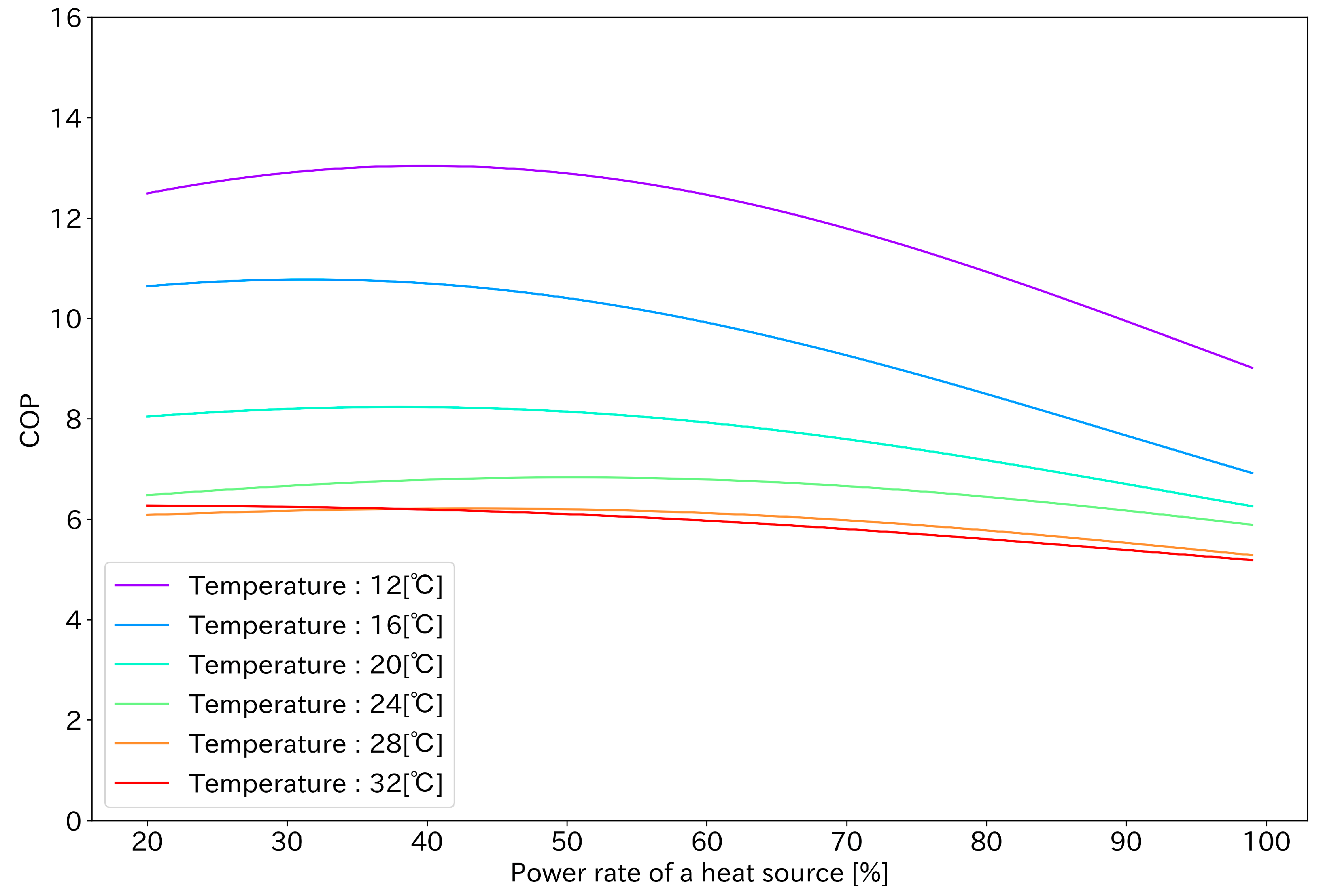
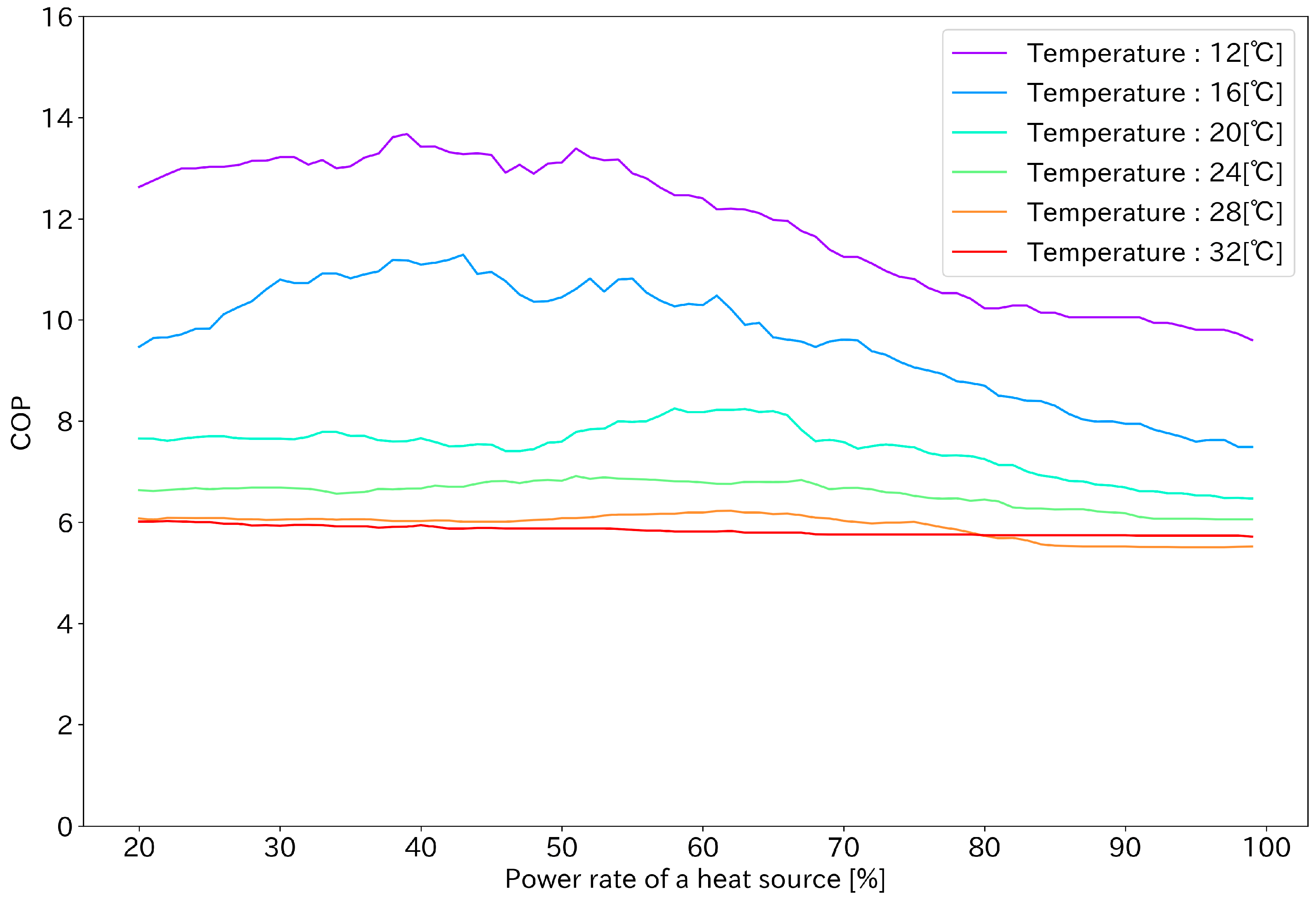
The COP is estimated for four chillers using one year of operating data. Chillers 1 and 2 are turbo chillers, and chillers 3 and 4 are inverter turbo chillers. The latter is characterized by a maximum COP at a load ratio of 30 to 40% when the temperature is low.
These four chillers were modeled and evaluated with k-partition cross-validation (k = 10), and the results are shown in Table 3, Table 4, Table 5 and Table 6, respectively. The error indices are MAE: Mean Absolute Error, RMSE: Root Mean Squared Error, and MAPE: Mean Percentage Error. Overall, the accuracy of SVR’s RBF kernel is relatively good. Next is the K-nearest neighbor method. Figure 4 and Figure 5 show the results of estimating the COP of chiller 4 using these two methods: Figure 4 with the SVR:RBF kernel shows a smooth line while Figure 5 with the K-nearest neighbor shows a line where the COP is not stable with respect to the output ratio. Although this function is used as a part of the objective function, the SVR: RBF kernel is used here because it is preferable to use smoother lines because unstable lines are more likely to lead to local solutions since the gradient information of the objective function is used to solve the optimization problem.
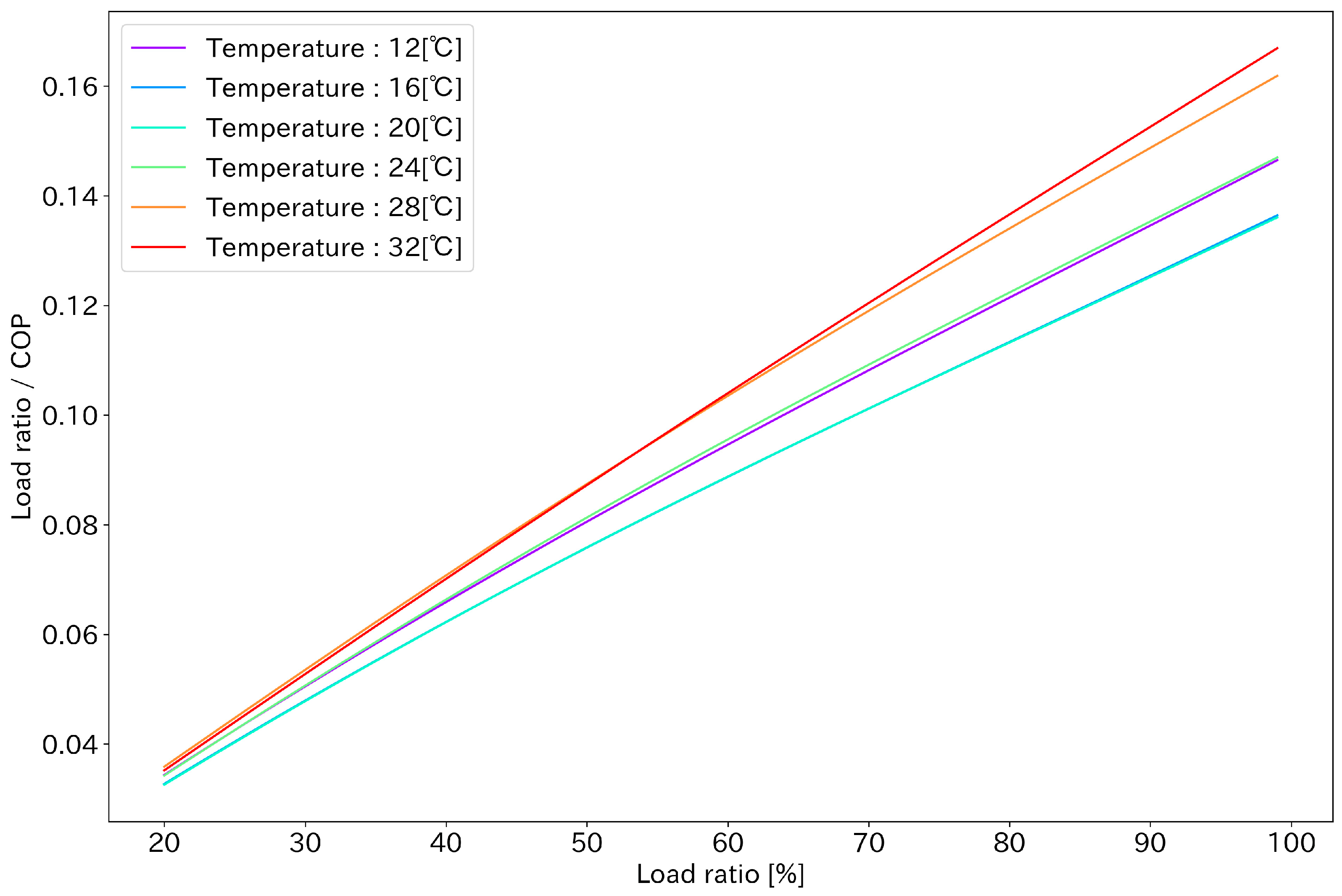
Assuming that increasing the output ratio r i , t increases the energy consumption, we mentioned that r i , t C O P i T t ,   r i , t in the objective function is a monotonically increasing function with respect to r i , t , but in reality, based on the estimated COP, when r i , t C O P i T t ,   r i , t was plotted, a monotonically increasing line was obtained as shown in Figure 6. Optimization can be performed for this COP function using a gradient-based optimization method.

3.3. Case Study of a Heat Source Equipment Operation Planning Method Considering COP Variation

The actual operation history is compared with the cost of operation using the planning method, which takes into account the variation of the COP using the proposed method, to verify how much cost reduction can be achieved by the proposed method. The learned COP model estimated previously is used, and Table 7 shows the results of power consumption reduction by the proposed method in the case of the COP model SVR. The actual power consumption of the actual chiller operation (“Actual” in the table) and the power consumption based on the estimated COP model (“Actual: COP Adjusted” in the table) are set as the comparison targets. “Actual after COP Adjustment” is prepared. “Actual after COP Adjusted” is intended to ensure the equality of the comparison since the energy consumption from the proposed method is calculated based on the estimated COP. For example, if the estimated COP function is inaccurate, and the COP is estimated to be higher than it should be, the power consumption in the “Proposed Method” will be improperly evaluated as small. To solve this problem, the “Actual after adjustment for COP” is calculated by dividing the chiller output by the estimated COP and comparing it with the “Proposed Method”. Although PV power generation forecasts, heat demand forecasts, and energy price forecasts are required to develop an actual operational strategy, here, for the sake of proof of concept, forecast values are assumed to be actual values for simplicity. The results for the actual and COP-adjusted results also show that the proposed method can reduce the electricity consumption by approximately 4% per year. Calculated at 14 yen/kWh, this amounts to about 4.1 million yen per year. Table 8 shows the results of power consumption reduction by the proposed method in the case of the COP model KNN. As shown in Table 9, KNN takes about three times longer to calculate the plan than the COP model SVR. This may be due to the fact that the COP estimation function with KNN is multimodal, which causes the gradient-based SLSQP calculation to fall into a local solution. It is also thought that the computation took longer for the same reason.
The specific operational schedules generated are examined here. 
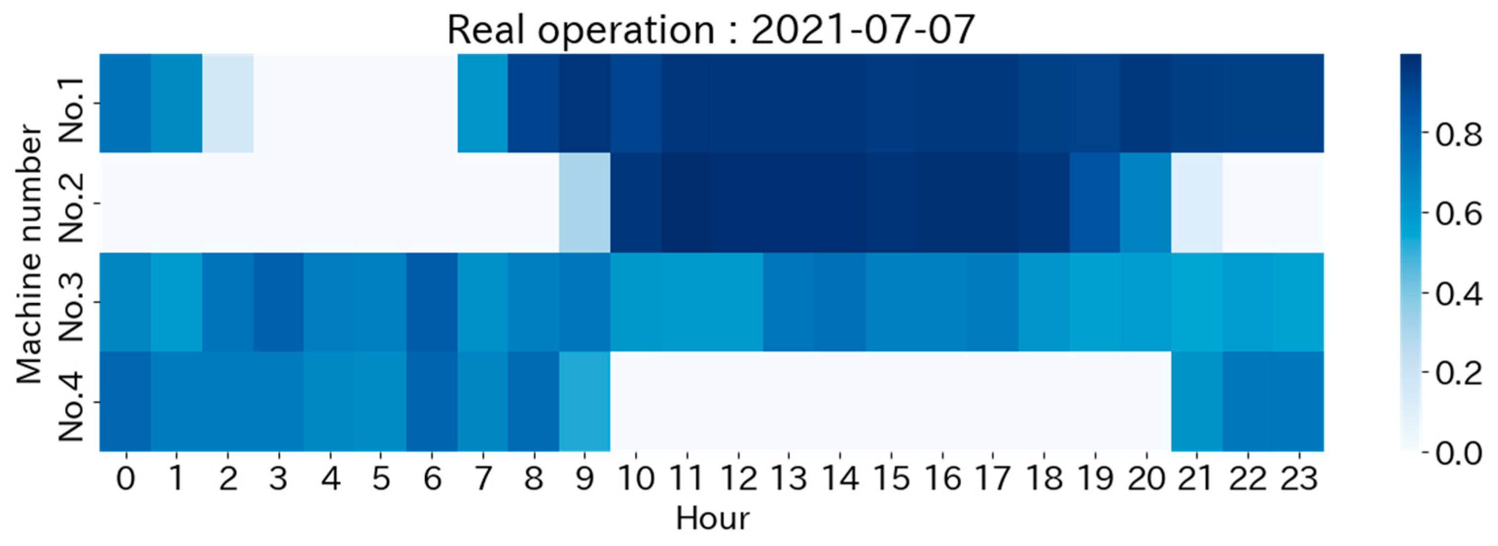
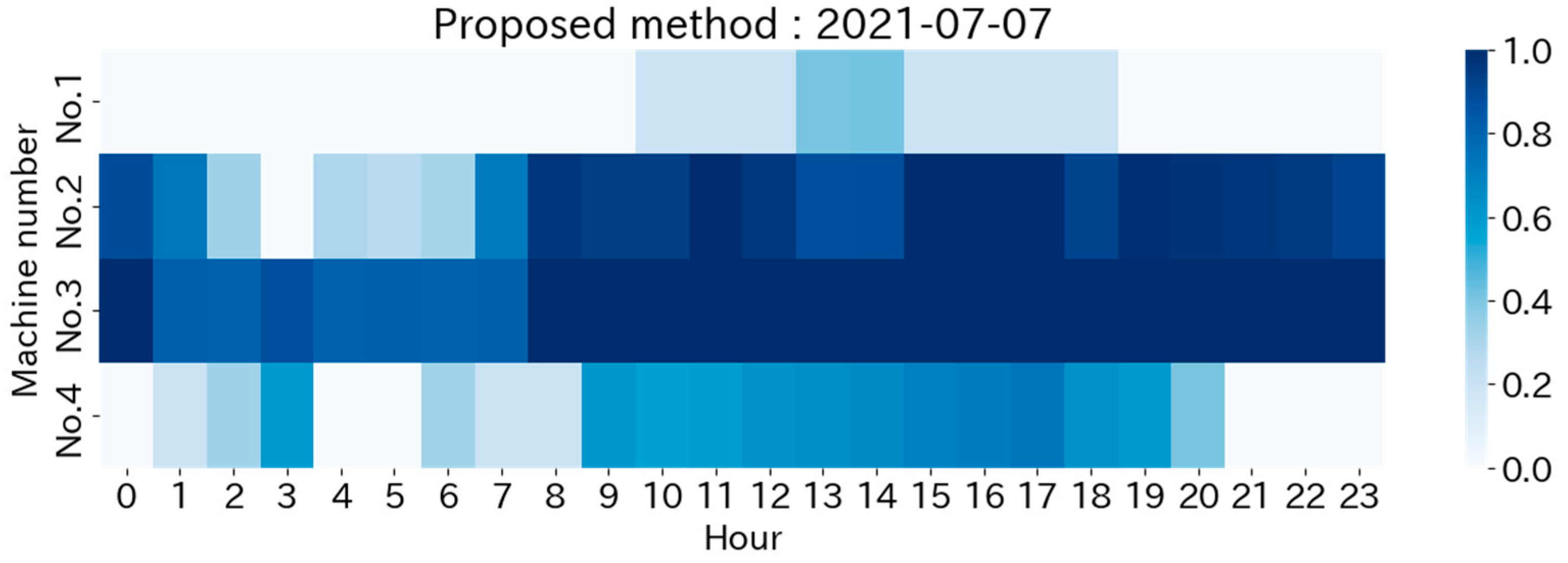
Figure 7 presents the operational schedule for a given day while
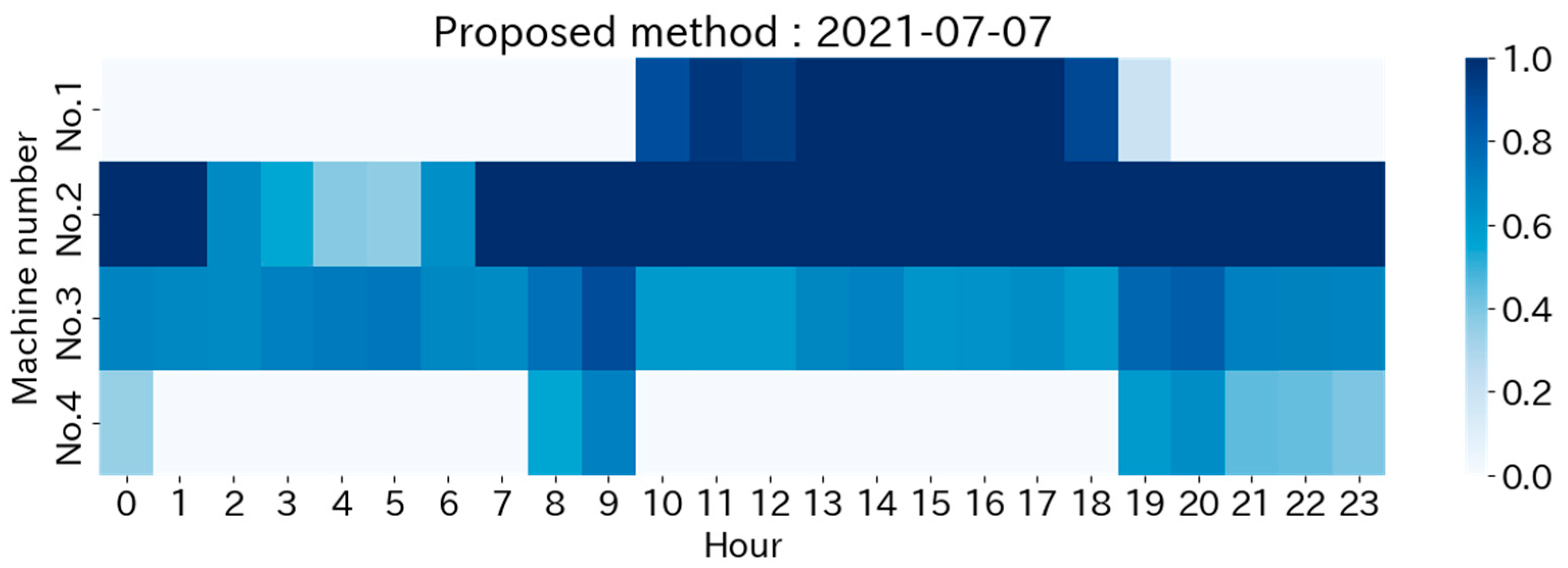
 Figure 8 and Figure 9 depict the schedules proposed by our methodology with the SVR and KNN COP models, respectively, for the same day. The color scheme in these figures indicates the ratio of operation intensity to maximum output.
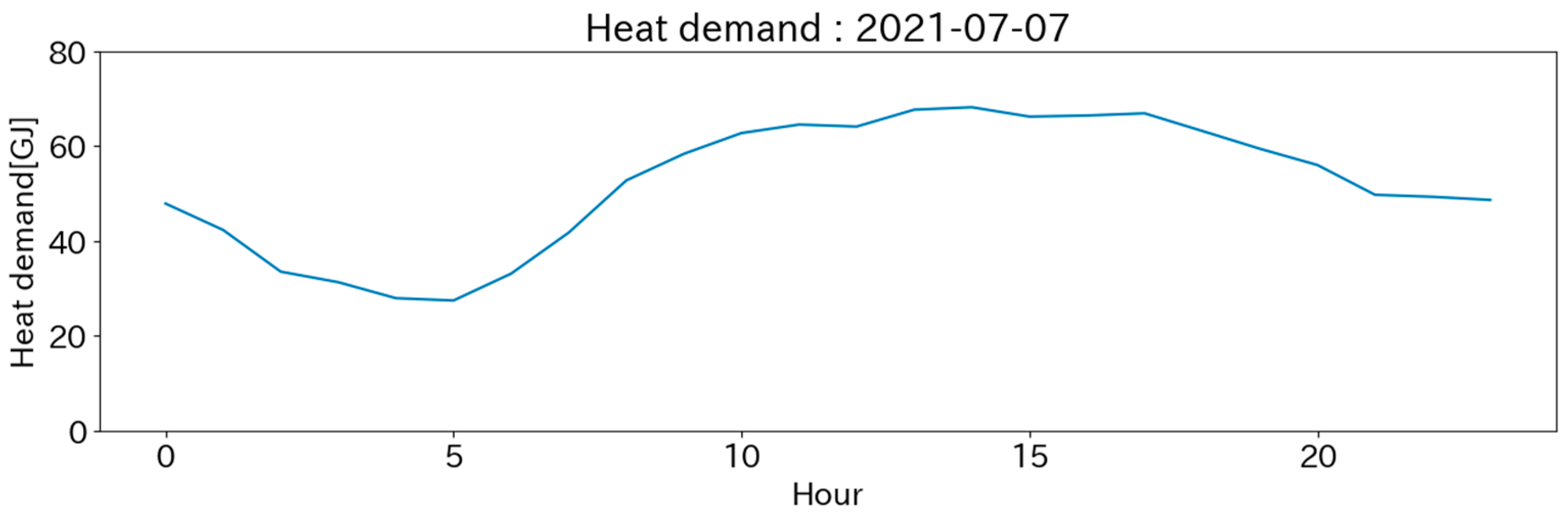
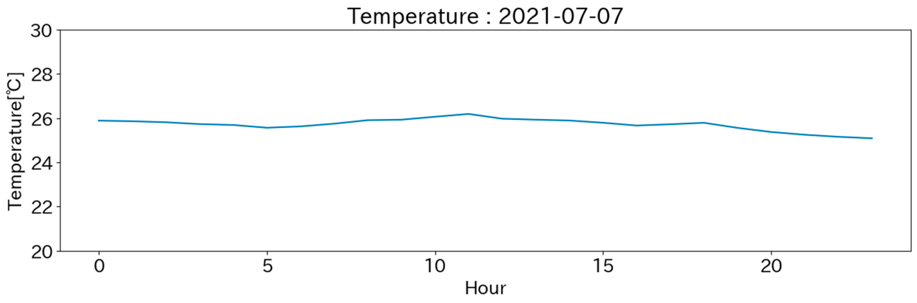
 Figure 10 and Figure 11 show the heat demand and temperature variations, respectively, for the same day. As can be inferred from Figure 7, the actual operation bases itself on chiller No.3, adjusting the operation of other chillers in line with the heat demand changes. However, the proposed operation schedule based on the SVR COP model, as shown in Figure 8, operates primarily on chillers No.2 and No.3. The main difference appears in the comparatively smaller demand period of late night to early morning. While the actual operations mainly involve chillers No.3 and No.4, with chiller No.1 serving as a supplement, the proposed methodology instead primarily operates chillers No.2 and No.3, with No.4 serving in a supplementary capacity. 
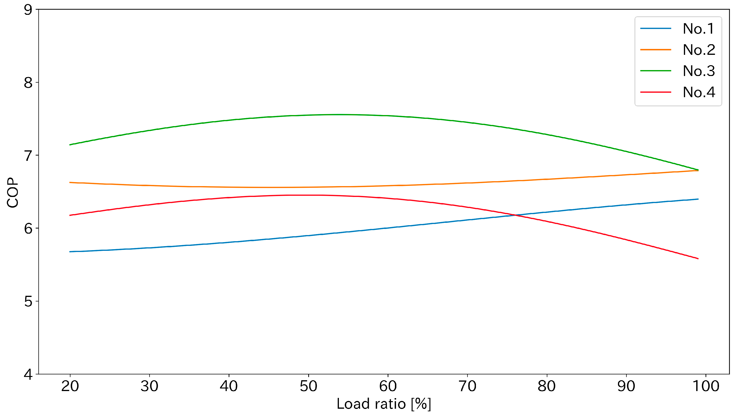
Figure 12 presents the COP curves of each chiller at a temperature of 26 degrees. Here, chiller No.3 consistently exhibits the highest COP, followed closely by No.2. Hence, based on the COP estimated from the data, it is rational under these weather conditions to prioritize chiller No.2 over No.4. This reasoning is reflected in the schedule generated by our proposed methodology. Moreover, chiller No.4 is more efficient than No.1 when the output ratio is small, but this is reversed around a 75% output ratio. Thus, under these weather conditions, there is a need to switch between chillers No.1 and No.4 according to the heat demand size. Our proposed method prioritizes chiller No.1 when the daytime heat demand is high and then switches to chiller No.4 in the evening when the heat demand decreases, demonstrating rational decision-making. It is difficult to consider both weather conditions and output ratio simultaneously in operations based on intuition and experience. Therefore, a scheduling methodology, such as our proposed one, which is based on an equipment efficiency model derived from actual data, is effective.

3.4. Case Study of an Operational Planning Method Capable of Exploring Trade-Offs between Environmental and Economic Performance

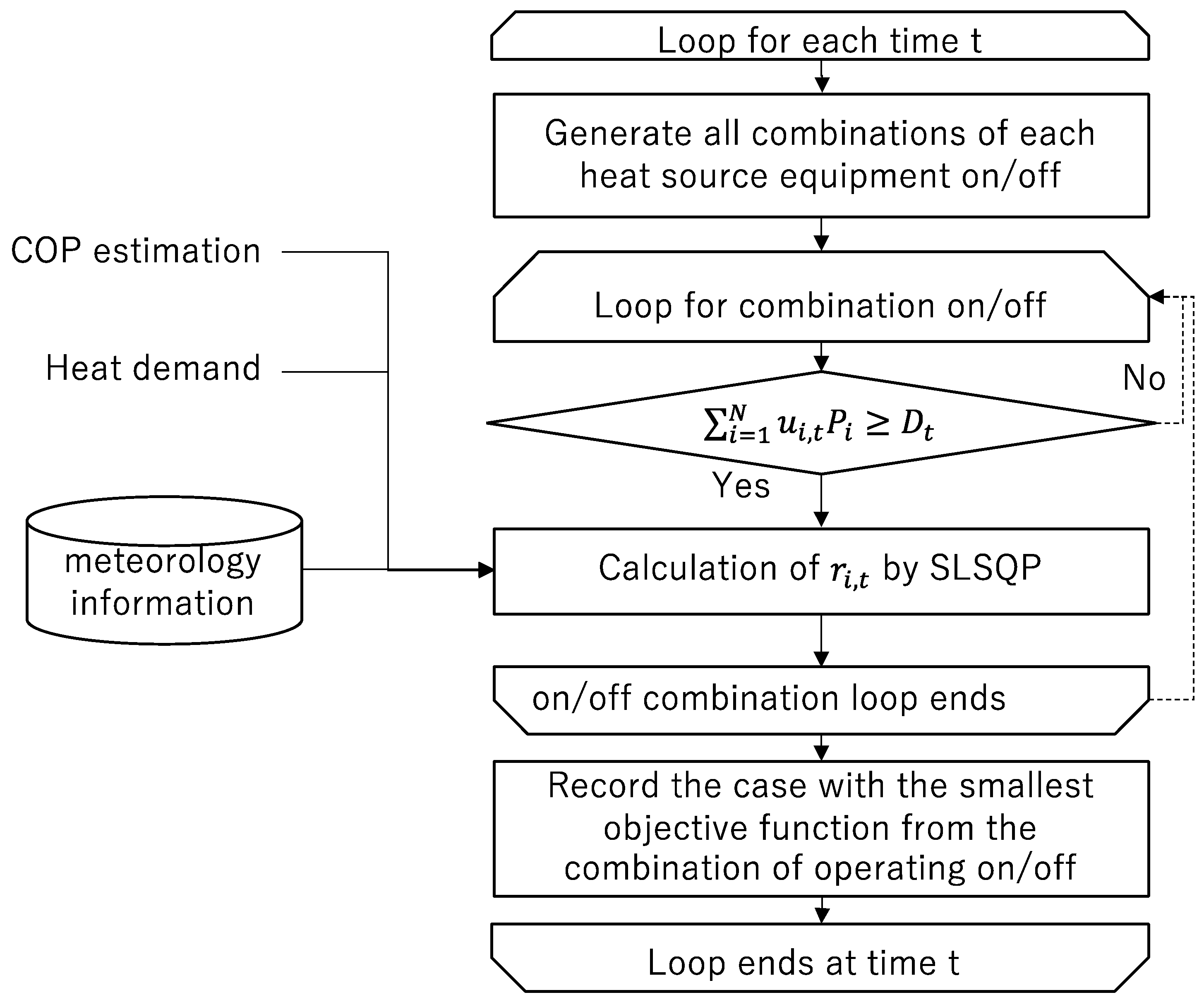
In this section, we conduct a multi-objective optimization comparison using two methods. The first method, depicted in 
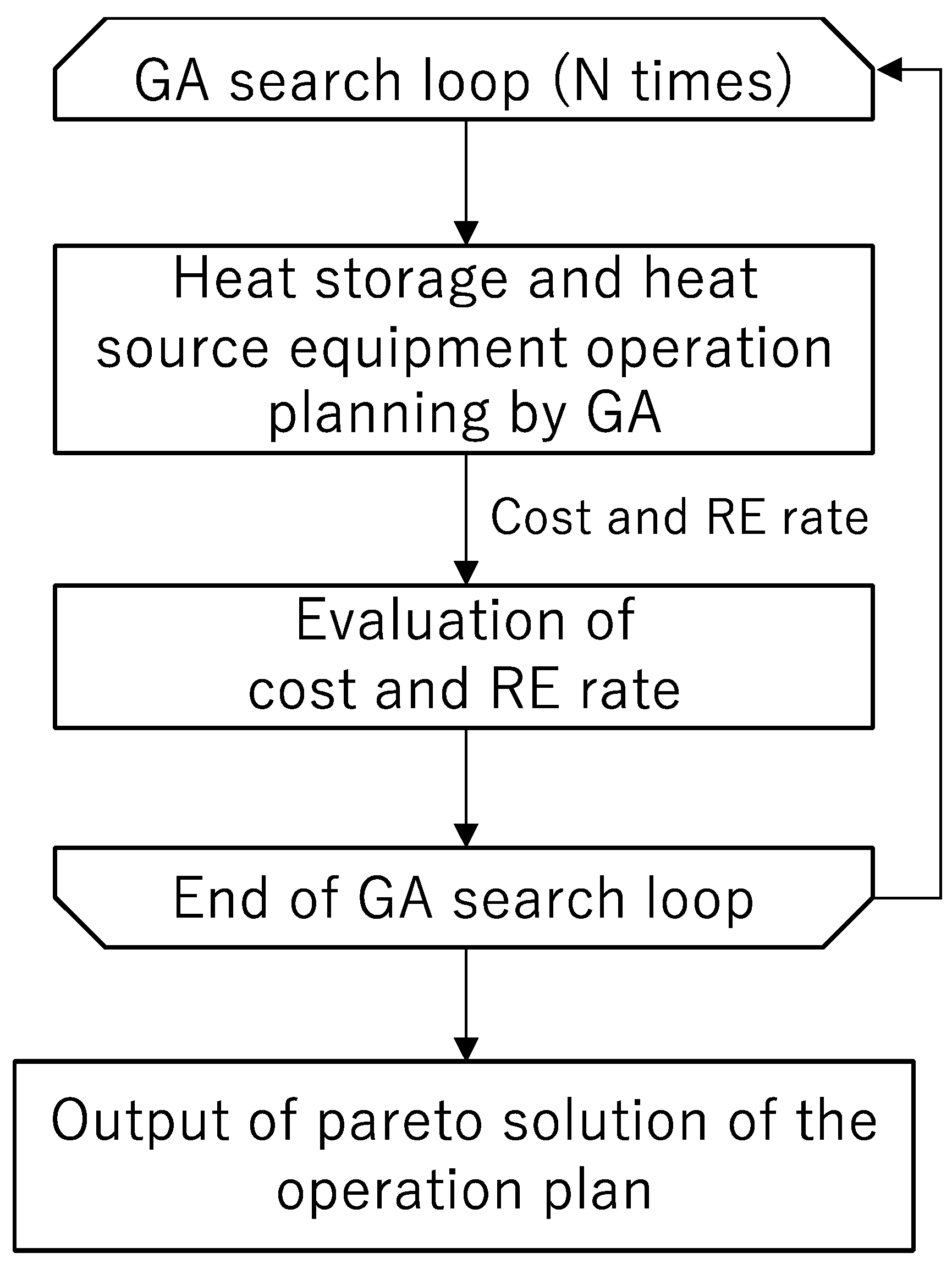
Figure 2, uses the GA exclusively to decide on the heat storage and release plan, along with the output plan for each heat source equipment. The second method, represented in 
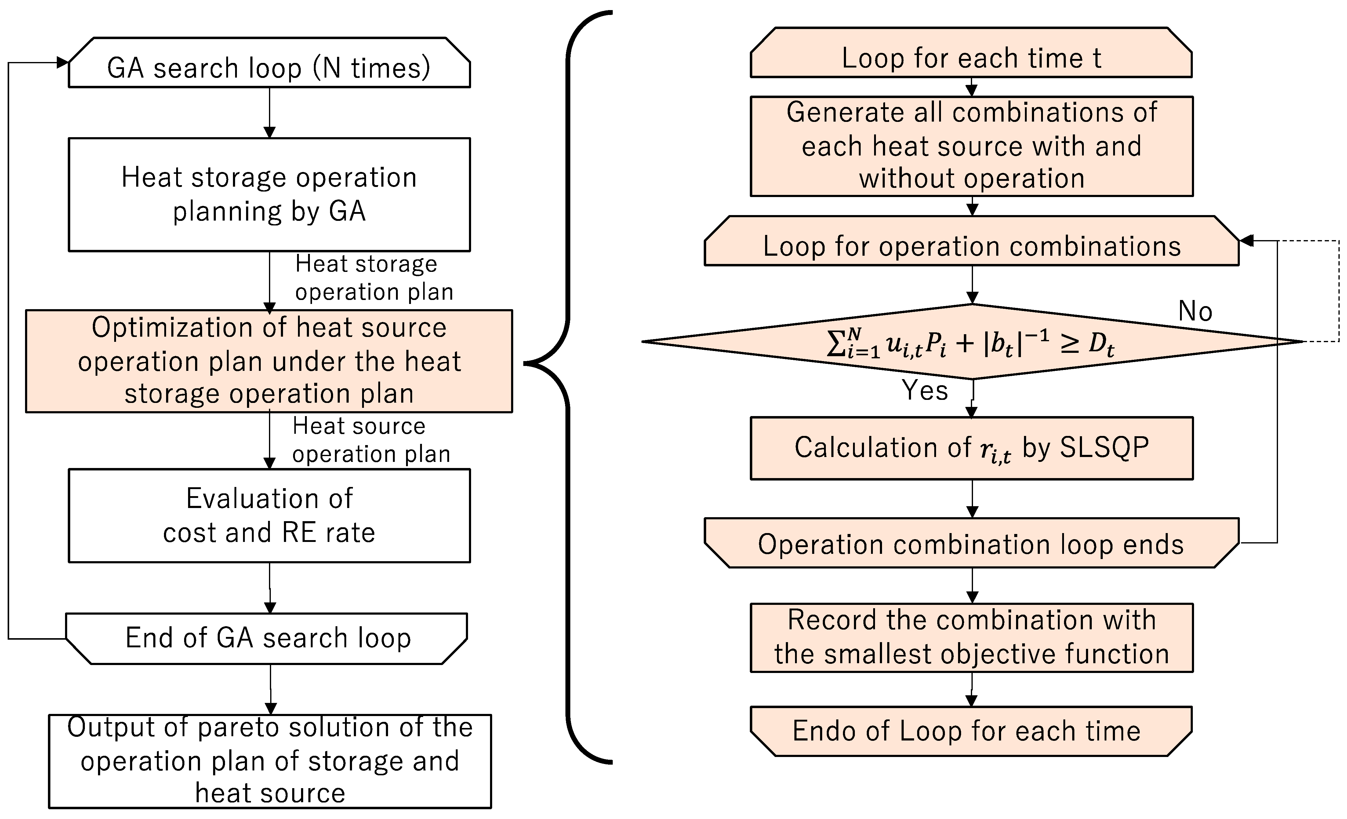
Figure 3 employs a two-stage optimization approach. Table 10 lists the set values of the constants used in this case study. We assume a scenario where the price of power purchased from the retail business remains consistent at 14 JPY/kWh, regardless of the time of day. As for the rate when selling surplus power generated by the PV system, we have considered the purchase price by a retail business for non-FIT (Feed-In Tariff) power. We assumed that 12 MW of PV was installed.
We examine how the Pareto front changes when altering the number of exploratory steps for two optimization techniques. 
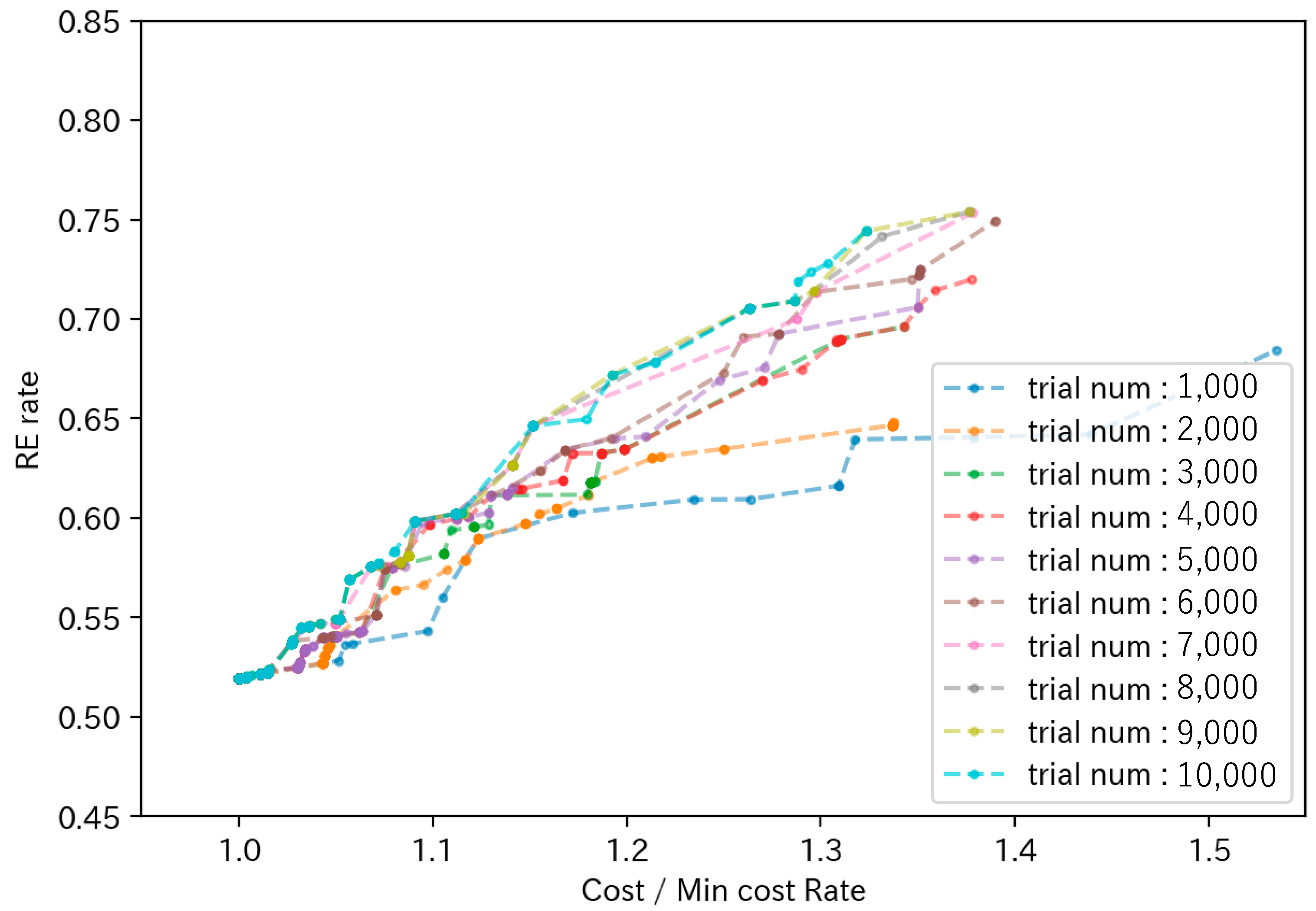
Figure 13 depicts the evolution of the Pareto front using a method that solely utilizes the Genetic Algorithm (GA). Multiple heat storage and release plans, along with operation plans for a given day, are plotted with the Renewable Energy (RE) rate on the y-axis and the cost ratio (minimized power consumption cost divided by total cost) on the x-axis. As the number of explorations increases, the Pareto front shifts towards the upper left, indicating an improvement with higher RE rates and lower costs. Until 3000 explorations, the Pareto front significantly improves, and after this point, the improvements gradually continue as the number of explorations increases. Beyond 7000 explorations, however, there seems to be little improvement. 
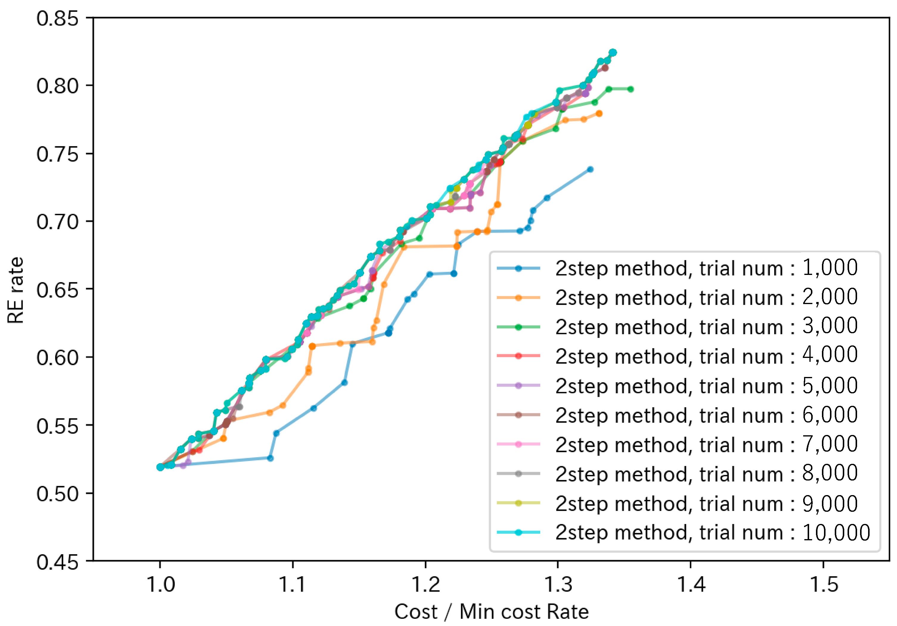
Figure 14 illustrates the evolution of the Pareto front using a two-stage optimization method. Compared to Figure 13, the Pareto front is positioned more towards the upper left overall, indicating superior exploratory performance. Additionally, until 3000 explorations, the Pareto front significantly improves, then it converges, demonstrating the two-stage optimization method’s efficiency per exploration.
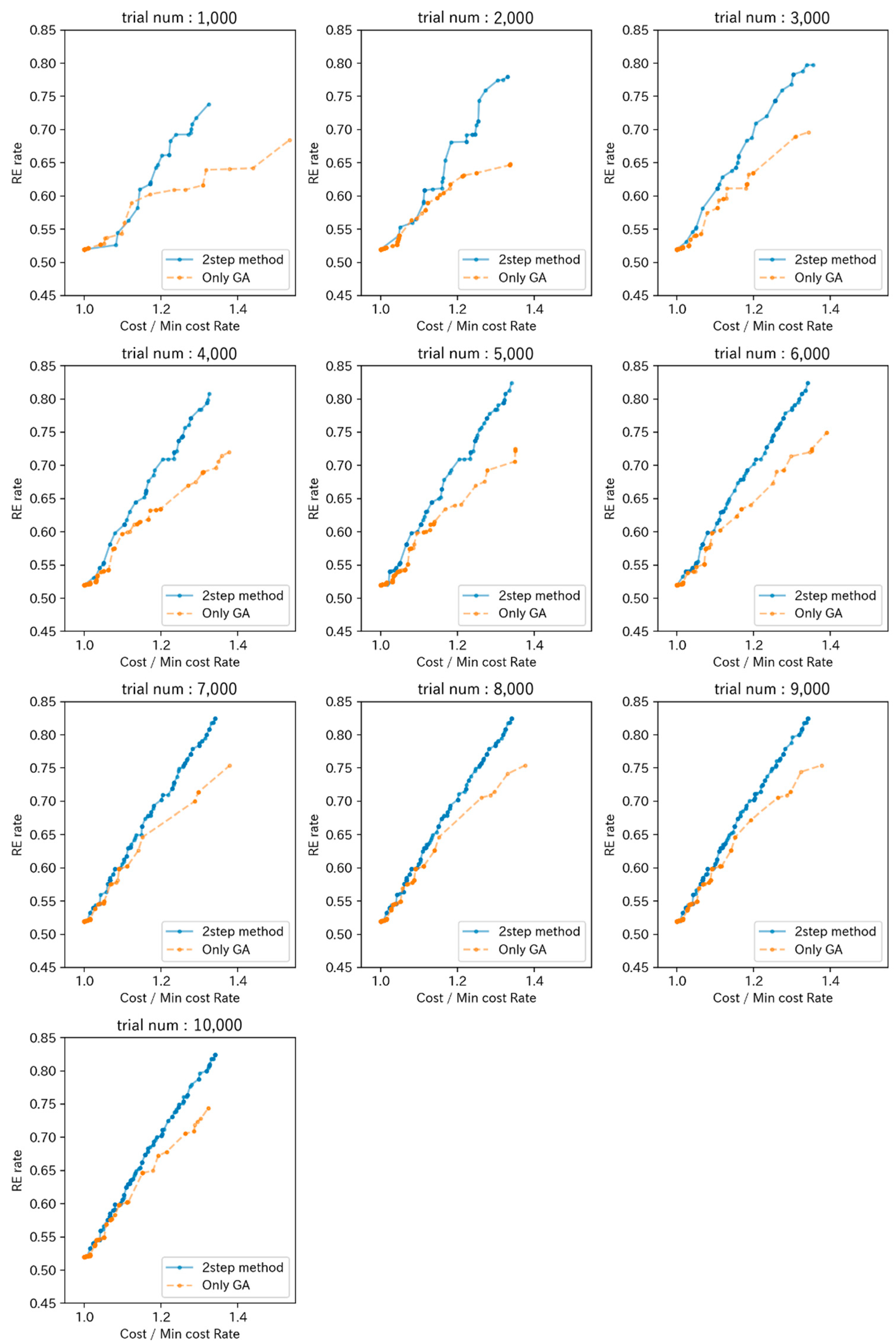
To compare and evaluate the differences between the Pareto solutions calculated by the two methods at the same search count, Figure 15 illustrates the Pareto solutions for both methods for search counts ranging from 1000 to 10,000. As depicted in the figure, the two-stage optimization method (labeled “2 step method” in the figure) generally positions the Pareto curve to the upper left more so than the method using only the GA (labeled “Only GA” in the figure). This demonstrates that the two-stage optimization method can achieve a higher RE ratio at a lower cost.
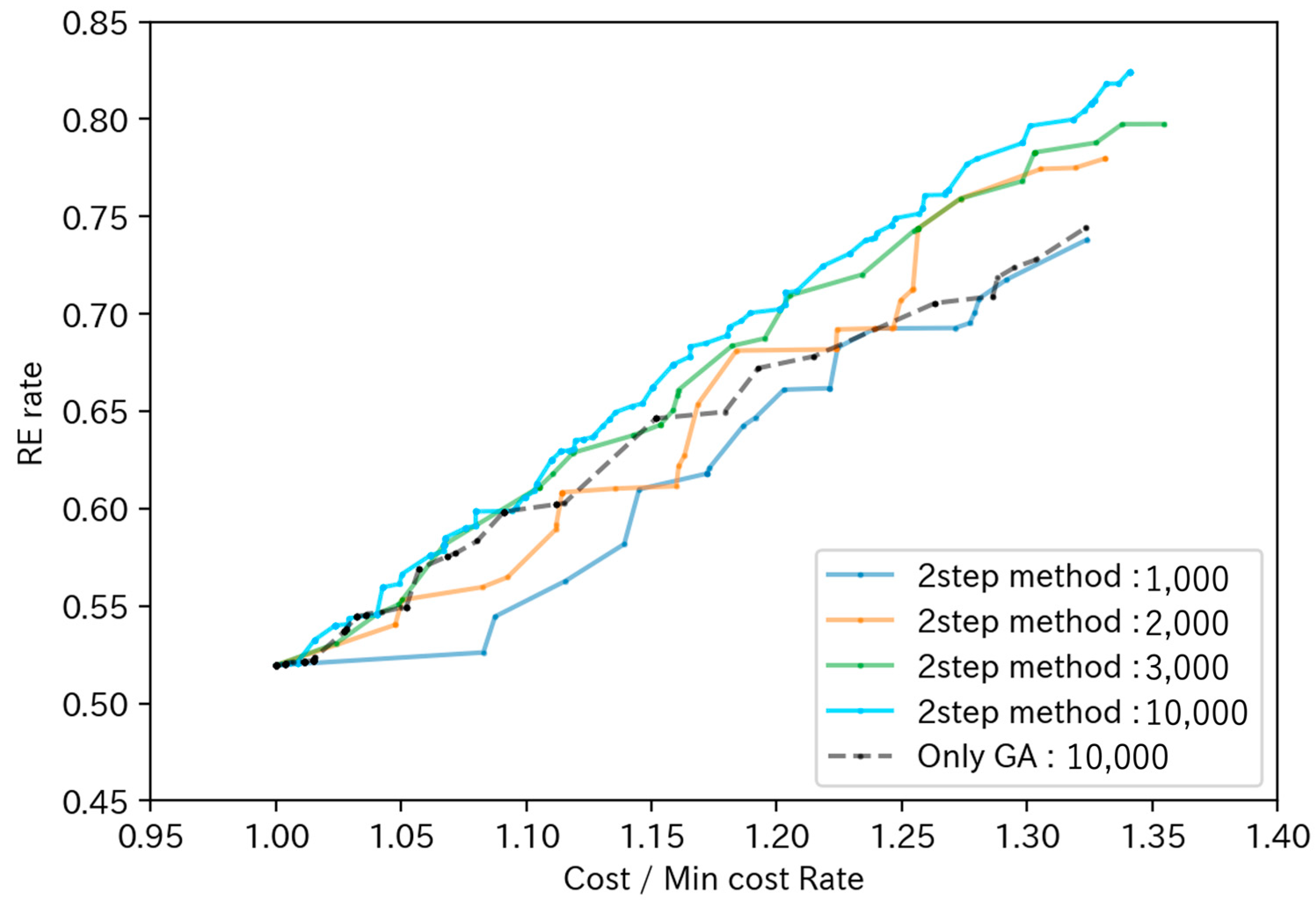
Figure 16 illustrates the Pareto frontiers for the method using only the Genetic Algorithm (GA) after 10,000 searches (represented by the black dotted line in the figure), and the two-stage optimization method after 1000 (blue), 2000 (orange), 3000 (green), and 10,000 (light blue) searches. As can be observed, the Pareto frontier obtained after 3000 searches using the two-stage optimization method (represented by the solid green line in the figure) is positioned further to the upper left compared to the frontier achieved after 10,000 searches using the GA-only method. This indicates that the two-stage optimization method can generate superior Pareto frontiers with fewer search iterations.
In the method using only the GA, 10,000 searches take 5766 s, averaging 0.577 s per search. Conversely, the two-stage optimization method takes 12,293 s for 10,000 searches, averaging 1.23 s per search. This is approximately 2.13 times the time per search. This increased time is due to the two-stage processing of the algorithm, involving GA search and optimization through Sequential Least Squares Programming (SLSQP). However, as shown in Figure 16, a better Pareto frontier is reached with 3000 searches using the two-stage optimization method than with 10,000 searches using only GA. In Table 11, 10,000 searches using the GA-only method take 5766 s while 3000 searches using the two-stage optimization method take 3761 s. This suggests that the two-stage optimization method can reach a superior Pareto frontier in just 65.2% of the time needed by the GA-only method. Despite the increased processing time per search, the two-stage optimization method demonstrates superior efficiency in a Pareto frontier search per unit of time because it can arrive at better solutions with fewer searches compared to the GA-only method.
Next, we will examine the details of the solutions produced by the two-stage optimization method. 
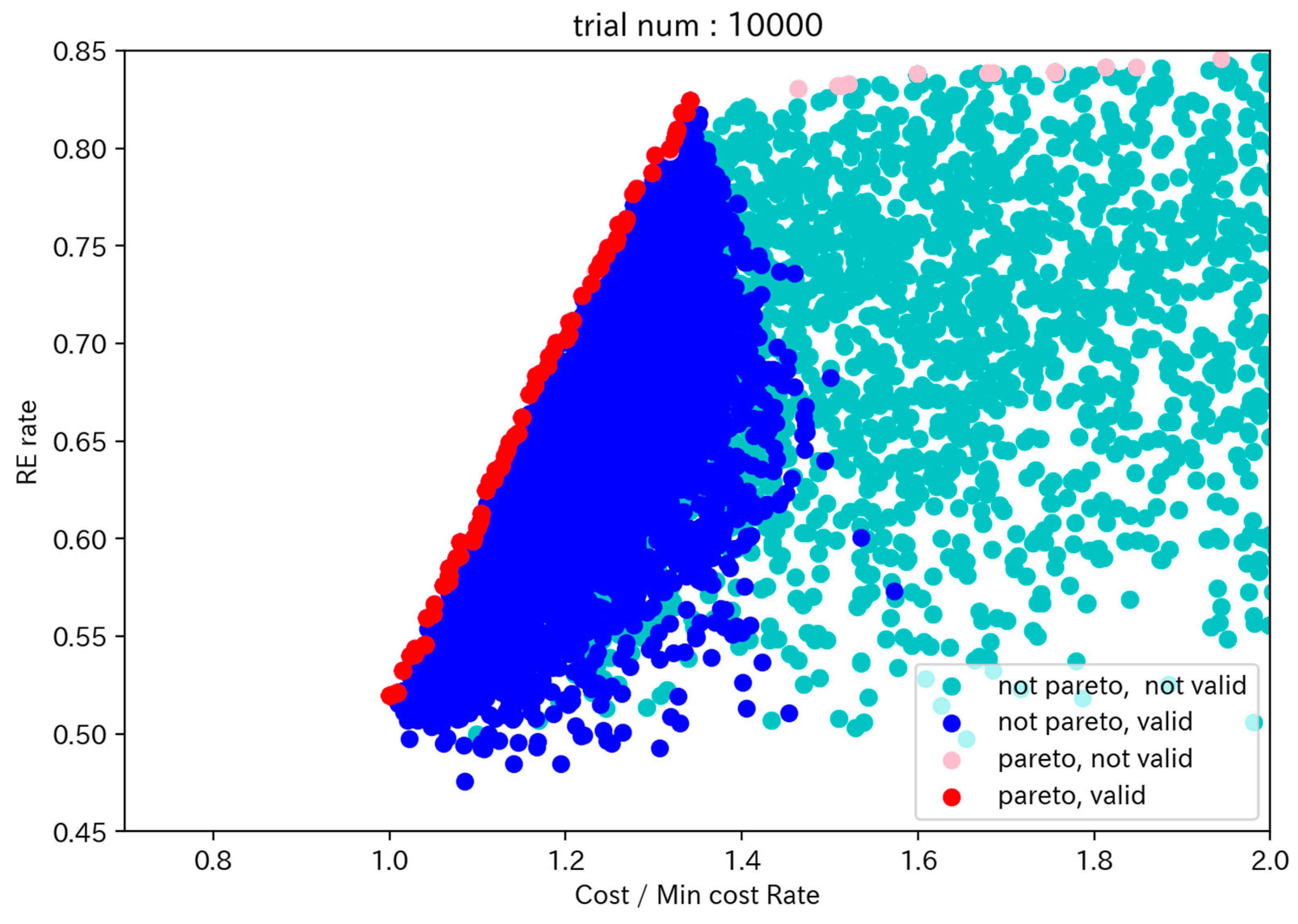
Figure 17 includes a plot of the results of 10,000 searches using the two-stage optimization method, including both Pareto-optimal solutions and sub-optimal solutions (those that are not Pareto-optimal). The color of the points represents red points for Pareto-optimal solutions that satisfy the constraints, light red points for Pareto-optimal solutions that do not satisfy the constraints, blue points for sub-optimal solutions that satisfy the constraints, and light blue points for sub-optimal solutions that do not satisfy the constraints. Here, the points representing the non-use of heat storage devices indicate the lowest cost solutions. This suggests that under these price settings, running the heat storage device is generally unprofitable due to the low Coefficient of Performance (COP) of the heat storage device. Furthermore, under this setting, where the price of electricity purchased from the retailer remains constant regardless of the time of day, there is no cost reduction effect through demand shifting by using heat storage devices. Similarly, under these pricing conditions (electricity sale price and purchase price), selling surplus PV power generated by the user to the retailer is more economical than storing it. Hence, there is no cost reduction effect through the utilization of surplus PV. Therefore, the pattern of not operating the heat storage device is the most economical. In the Pareto-optimal solutions that satisfy the constraints (represented by red points), the cost and RE rate rise at almost a constant ratio. When the RE rate reaches around 82%, there are no longer any Pareto-optimal solutions that satisfy the constraints. From the Pareto-optimal solutions satisfying the constraints (red points), one would select the heat storage and dissipation schedule and the operation schedule for each heat source device. The Pareto point with the lowest cost is (cost ratio, RE rate) = (1.00, 0.52) and the Pareto point with the highest RE rate is (cost ratio, RE rate) = (1.34, 0.82). In other words, it is found that if a cost increase of 34% is permitted, the RE rate can be improved by about 30%.
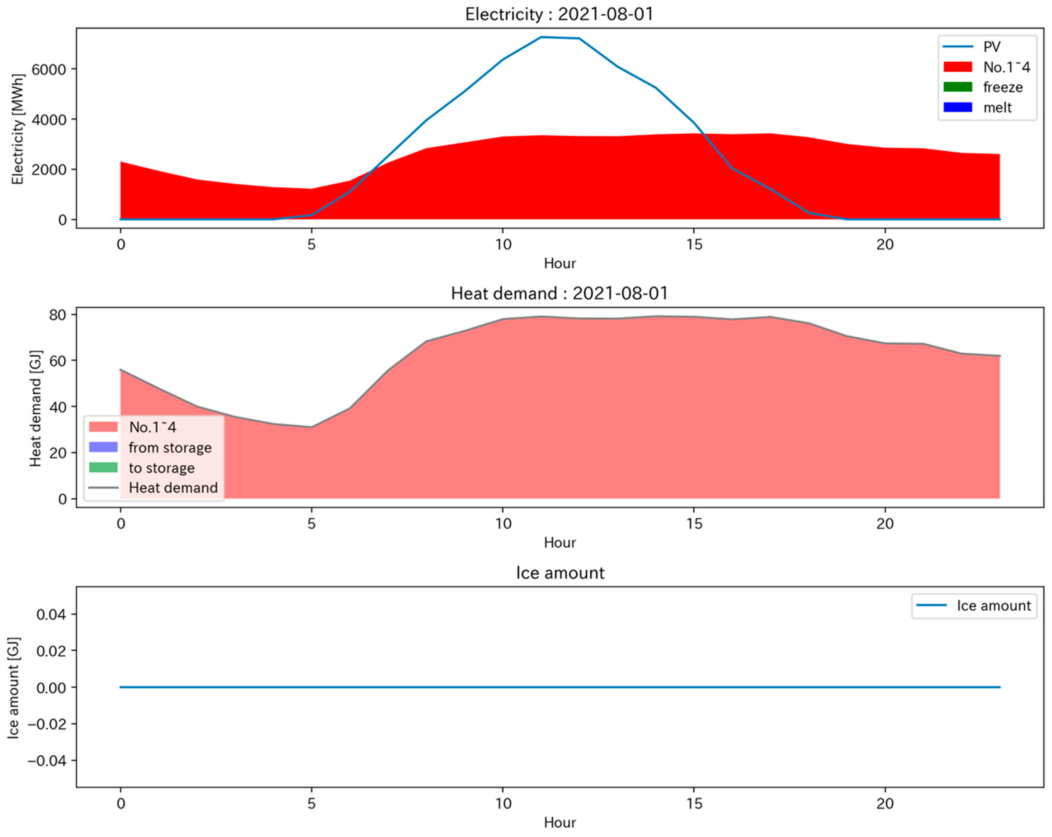
Figure 18 shows the power consumption, heat supply, and heat storage in the operation plan for the cost-saving oriented point (cost ratio, RE rate) = (1.00, 0.52). 
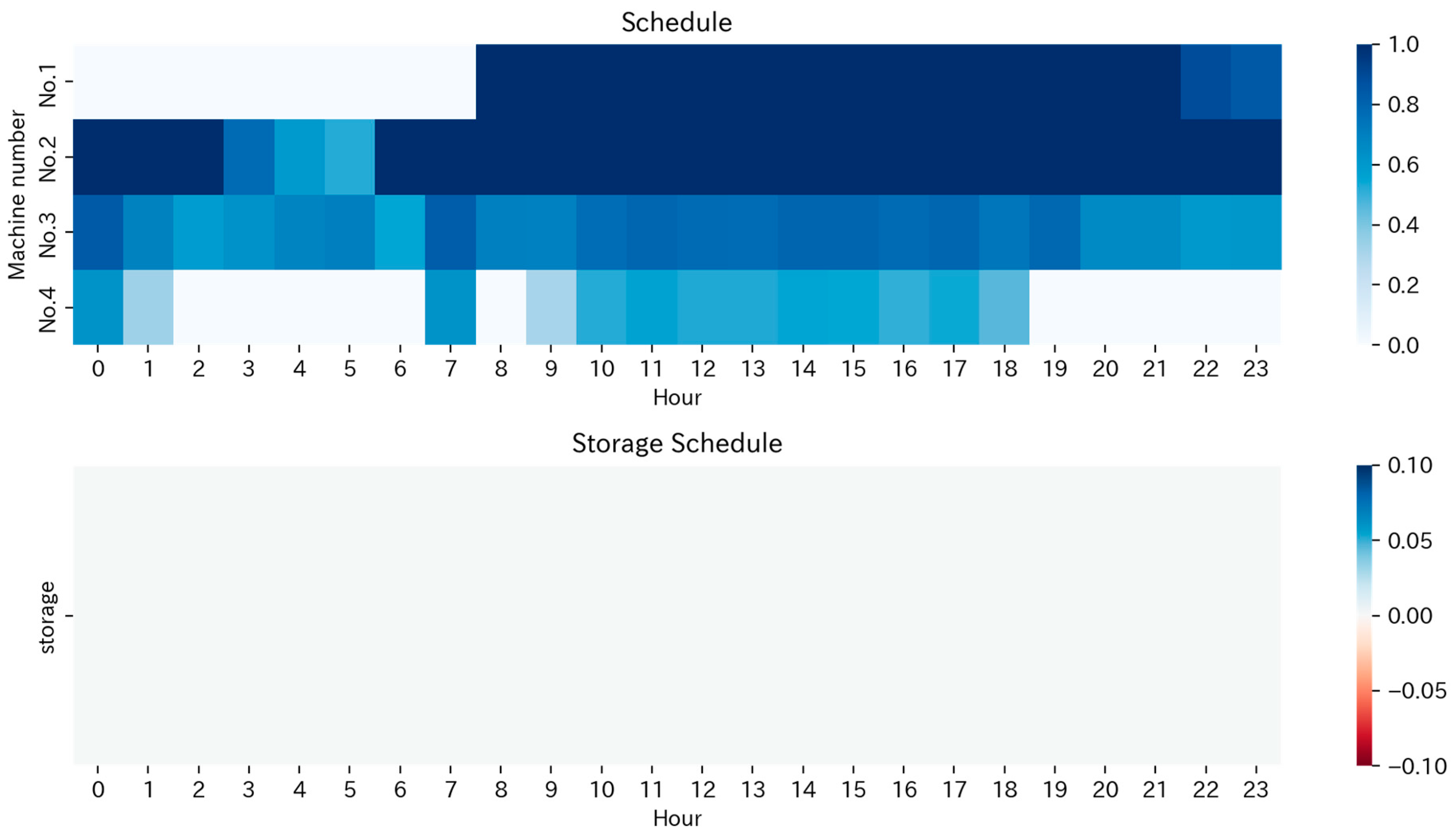
Figure 19 shows the operating schedule of the heat source equipment No.1 to 4 and the heat storage device under the same cost-saving oriented plan. There is no heat storage or dissipation, and heat demand is met solely through the operation of the heat source equipment.
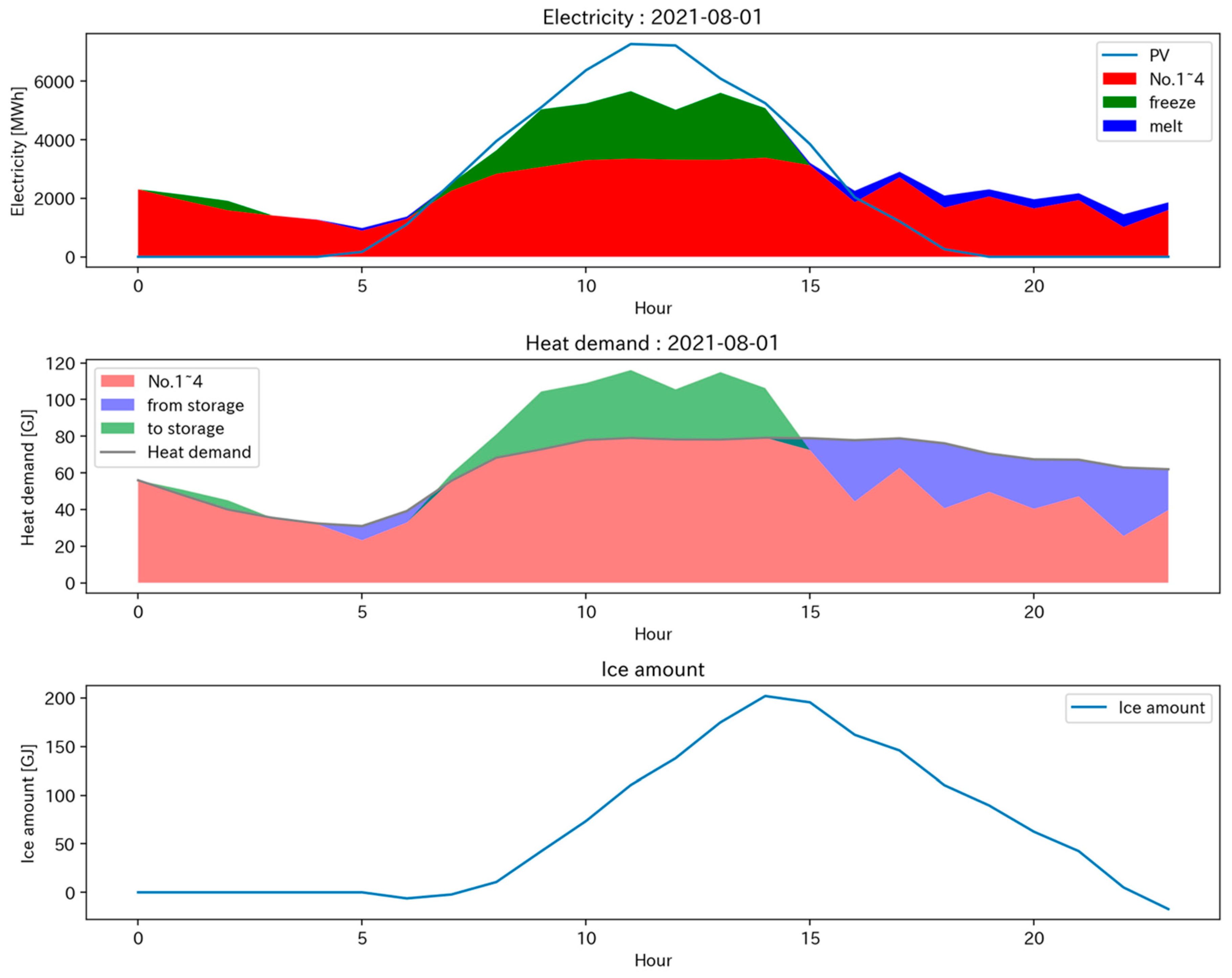
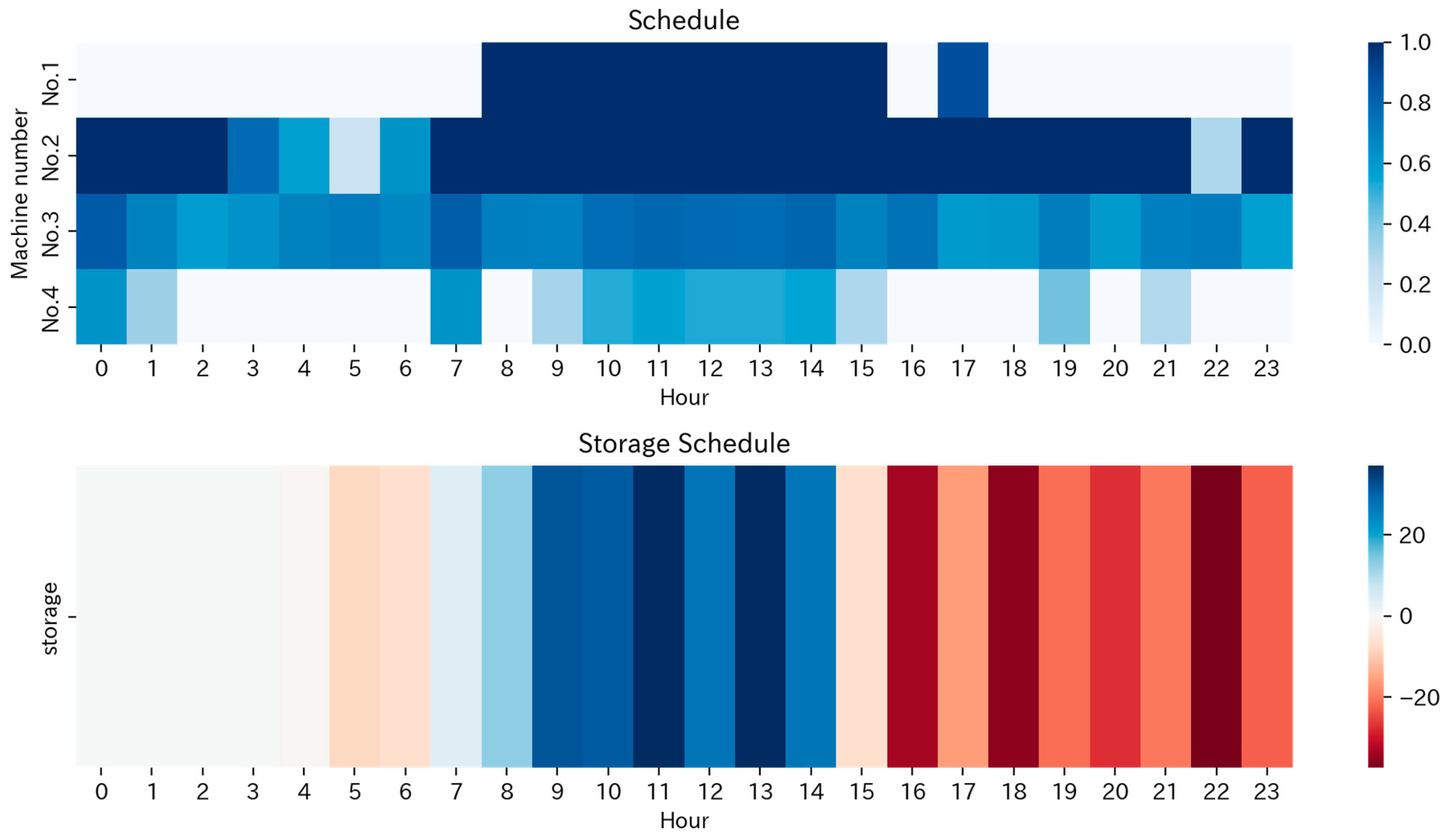
Figure 20 shows the power consumption, heat supply, and heat storage in the operation plan for the renewable-energy oriented point (cost ratio, RE rate) = (1.34, 0.82). It can be seen that surplus PV during the day is stored up to the maximum amount of ice that can be stored, and heat dissipation begins from the evening when the surplus power generation ceases. Although a slight amount of heat storage can be observed around 1–2 am, it does not contribute to improving the renewable energy ratio, nor does it contribute to cost reduction. Therefore, this is not an optimal strategy and suggests that there is room for further exploration of solutions. Figure 21 shows the operating schedule of the heat source equipment No.1 to 4 and the heat storage device for the same Pareto point. Considering the amount of heat supplied by heat dissipation from evening to night, the operating level of the heat source equipment is confirmed to be lower than that in Figure 19. Moreover, 
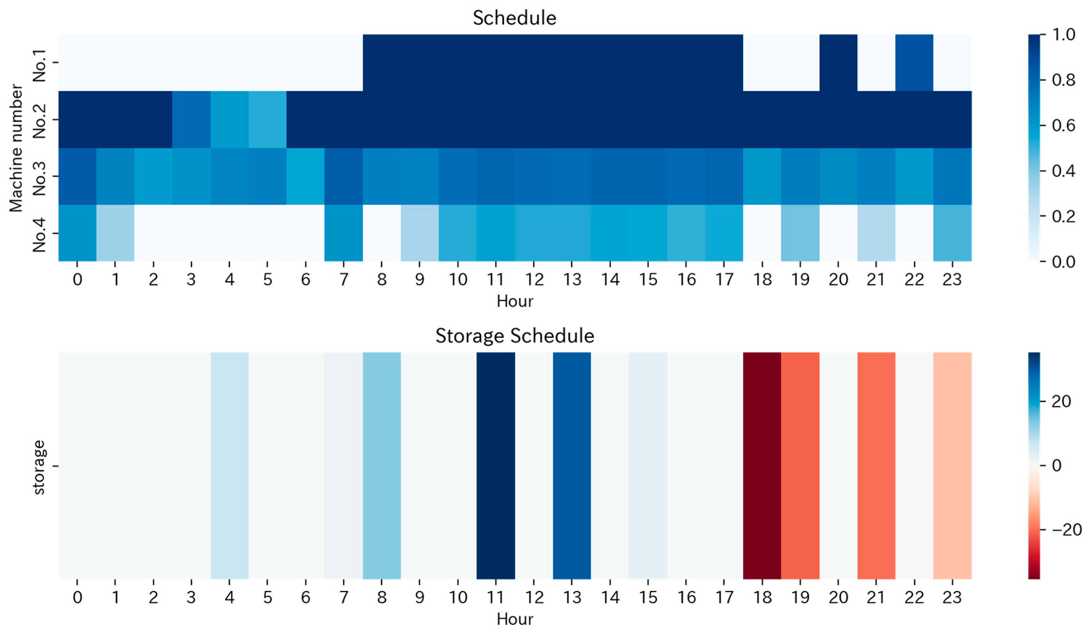
Figure 22 presents the power consumption, heat supply, and heat storage in the operation plan for a point with a balance between the cost and renewable energy orientation (cost ratio, RE rate) = (1.15, 0.65). While it absorbs surplus renewable energy during the day, it does not store as much as the renewable-energy oriented plan. Figure 23 shows the operating schedule of the heat source equipment No.1 to 4 and the heat storage device for the same cost-renewable energy balance oriented plan. The amount of heat dissipation at night is not as significant as in the renewable-energy oriented plan.
By deriving Pareto solutions from multi-objective optimization, it is possible to determine the heat storage and dissipation strategy and the operation plan of the heat source equipment that an entity should adopt according to the entity’s orientation, be it cost-saving, renewable-energy, or cost-renewable energy balance oriented.

4. Conclusions

In this study, we constructed a system to support the decision-making process of entities owning renewable energy generation facilities by calculating Pareto solutions through a multi-objective optimization that balances economic and environmental objectives. We adopted a non-parametric COP estimation method using machine learning, and by integrating the estimation function into the optimization formula, we achieved a more realistic and flexible system modeling, demonstrating that an approximate annual cost reduction of 4% is possible from the current operation. Moreover, when adding a thermal storage facility, we set the proportion of renewable energy in power consumption as the RE rate, an environmental index and the electricity bill as an economic index.
By solving the multi-objective optimization of operation strategies with these as objective functions, we were led to Pareto solutions and constructed a model for selecting operation strategies considering the balance of objective functions. Specifically, we proposed and compared methods for calculating solutions using only the GA and a two-step optimization method combining GA and SLSQP, confirming the superiority of the two-step optimization method. The case study unveiled unique operational profiles corresponding to cost-saving, renewable-energy, and balanced orientation points, suggesting the existence of specific strategies tailored to each orientation. As a result, we built a model that allows stakeholders to select daily operation strategies according to their preferences.
It should be noted that the optimization method used here is based on the genetic algorithm, and its optimality is not guaranteed; hence, there is a possibility that better Pareto solutions may exist.

5. Future Work

One limitation of this method is that it may require approximately a year’s worth of data to train a model that can estimate the Coefficient of Performance (COP). However, the real value of this approach becomes evident when the manufacturer’s COP curve starts to diverge from reality over time due to deterioration or other factors. It is assumed that by this point, sufficient data will have been accumulated. If sufficient data cannot be prepared to train the COP model, it is still possible to carry out a subsequent optimization using the manufacturer’s COP curve as an alternative. In such a case, a future task would be to determine the extent to which this approach deviates from reality.
In addition, we aim to delve deeper into the optimization of parameters for our non-MLP models, including the SVR model. The parameters for these models were kept fixed in our current study. However, we recognize the potential impact that parameter optimization could have on the performance of these models. Specifically, for the SVR model, we will look into optimizing parameters like the regularization parameter ‘C’ and the kernel functions, which could significantly affect the model’s accuracy. We also plan to explore different kernels beyond the ‘rbf’ kernel used in this study. Moreover, we plan to extend our investigations to other machine learning models and optimization techniques. This would allow us to compare and contrast the effectiveness of various models and strategies, potentially leading to more robust and efficient solutions.
Lastly, we anticipate refining our data collection and handling methods. This would include obtaining more precise information about data quality and sensor accuracy, which can further enhance our model’s predictive ability and overall reliability.

Author Contributions

Conceptualization, D.S.; methodology, D.S.; software, D.S.; writing—original draft preparation, D.S.; project administration; K.T. All authors have read and agreed to the published version of the manuscript.

Funding

Grant-in-Aid for Scientific Research (A) 20H00285 from the Japan Society for the Promotion of Science (JSPS).

Data Availability Statement

Restrictions apply to the availability of these data. The data may be available from the authors, but only if permission is granted by Kansai Airports and Kansai International Airport’s Heating and Cooling Supply. However, obtaining this permission is not guaranteed.

Acknowledgments

This research project was carried out in cooperation with Kansai Airports. We would like to express our deepest gratitude to Kansai Airports for their helpful advice and to Kansai International Airport Heating & Cooling Supply for provision of their data. The second author is supported by Grant-in-Aid for Scientific Research (A) 20H00285 from the Japan Society for the Promotion of Science (JSPS).

Conflicts of Interest

The authors declare no conflict of interest.

References

  1. Hajiah, A.; Krarti, M. Optimal control of building storage systems using both ice storage and thermal mass-Part I: Simulation environment. Energy Convers. Manag. 2012, 64, 499–508. [Google Scholar] [CrossRef]
  2. Hajiah, A.; Krarti, M. Optimal controls of building storage systems using both ice storage and thermal mass-Part II: Parametric analysis. Energy Convers. Manag. 2012, 64, 509–515. [Google Scholar] [CrossRef]
  3. Lee, D.; Ooka, R.; Ikeda, S.; Choi, W.; Kwak, Y. Model predictive control of building energy systems with thermal energy storage in response to occupancy variations and time-variant electricity prices. Energy Build. 2020, 225, 110291. [Google Scholar] [CrossRef]
  4. Kim, D.; Wang, Z.; Brugger, J.; Blum, D.; Wetter, M.; Hong, T.; Piette, M.A. Site demonstration and performance evaluation of MPC for a large chiller plant with TES for renewable energy integration and grid decarbonization. Appl. Energy 2022, 321, 119343. [Google Scholar] [CrossRef]
  5. Kircher, K.J.; Zhang, K.M. Model predictive control of thermal storage for demand response. In Proceedings of the 2015 American Control Conference (ACC), Chicago, IL, USA, 1–3 July 2015; IEEE: New York, NY, USA, 2015; pp. 956–961. [Google Scholar]
  6. Oldewurtel, F.; Ulbig, A.; Morari, M.; Andersson, G. Building control and storage management with dynamic tariffs for shaping demand response. In Proceedings of the 2011 2nd IEEE PES International Conference and Exhibition on Innovative Smart Grid Technologies, Manchester, UK, 5–7 December 2011; IEEE: New York, NY, USA, 2011; pp. 1–8. [Google Scholar]
  7. Reynders, G.; Nuytten, T.; Saelens, D. Potential of structural thermal mass for demand-side management in dwellings. Build. Environ. 2013, 64, 187–199. [Google Scholar] [CrossRef]
  8. Abdelkader, A.; Rabeh, A.; Ali, D.M.; Mohamed, J. Multi-objective genetic algorithm based sizing optimization of a stand-alone wind/PV power supply system with enhanced battery/supercapacitor hybrid energy storage. Energy 2018, 163, 351–363. [Google Scholar] [CrossRef]
  9. Ould Bilal, B.; Sambou, V.; Ndiaye, P.A.; Kébé, C.M.F.; Ndongo, M. Optimal design of a hybrid solar–wind–battery system using the minimization of the annualized cost system and the minimization of the loss of power supply probability (LPSP). Renew. Energy 2010, 35, 2388–2390. [Google Scholar] [CrossRef]
  10. Yang, H.; Zhou, W.; Lu, L.; Fang, Z. Optimal sizing method for stand alone hybrid solar-wind system with LPSP technology by using genetic algorithm. Sol. Energy 2008, 82, 354–367. [Google Scholar] [CrossRef]
  11. Dufo-López, R.; Bernal-Agustín, J.L.; Yusta-Loyo, J.M.; Domínguez-Navarro, J.A.; Ramírez-Rosado, I.J.; Juan Lujano, J.; Ismael Aso, I. Multi-objective optimization minimizing cost and life cycle emissions of stand-alone PV wind–diesel systems with batteries storage. Appl. Energy 2011, 88, 4033–4041. [Google Scholar] [CrossRef]
  12. Saif, A.; Gad Elrab, K.; Zeineldin, H.H.; Kennedy, S.; Kirtley, J.L. Multi-objective capacity planning of a PV-wind-diesel-battery hybrid power system. In Proceedings of the IEEE International Conferences, Manama, Bahrain, 18–22 December 2010. [Google Scholar]
  13. Ascione, F.; Bianco, N.; De Masi, R.F.; De Stasio, C.; Mauro, G.M.; Vanoli, G.P. Multi-objective optimization of the renewable energy mix for a building. Appl. Therm. Eng. 2016, 101, 612–621. [Google Scholar] [CrossRef]
  14. Navidbakhsh, M.; Shirazi, A.; Sanaye, S. Four E analysis and multi-objective optimization of an ice storage system incorporating PCM as the partial cold storage for air-conditioning applications. Appl. Therm. Eng. 2013, 58, 30–41. [Google Scholar] [CrossRef]
  15. Lee, W.S.; Chen, Y.T.; Wu, T.H. Optimization for ice-storage air-conditioning system using particle swarm algorithm. Appl. Energy 2009, 86, 1589–1595. [Google Scholar] [CrossRef]
  16. Zhou, X.; Yu, J.; Zhang, W.; Zhao, A.; Zhou, M. A multi-objective optimization operation strategy for ice-storage air-conditioning system based on improved firefly algorithm. Build. Serv. Eng. Res. Technol. 2022, 43, 161–178. [Google Scholar] [CrossRef]
  17. Zhao, T.; Wang, J.; Xu, M.; Li, K. An online predictive control method with the temperature based multivariable linear regression model for a typical chiller plant system. Build. Simul. 2020, 13, 335–348. [Google Scholar] [CrossRef]
  18. Wei, X.; Xu, G.; Kusiak, A. Modeling and optimization of a chiller plant. Energy 2014, 73, 898–907. [Google Scholar] [CrossRef]
  19. Ren, Y.; Yu, J.; Zhao, A.; Jing, W.; Ran, T.; Yang, X. A multi-objective operation strategy optimization for ice storage systems based on decentralized control structure. Build. Serv. Eng. Res. Technol. 2021, 42, 62–81. [Google Scholar] [CrossRef]
  20. Zheng, X.; Wu, G.; Qiu, Y.; Zhan, X.; Shah, N.; Li, N.; Zhao, Y. A MINLP multi-objective optimization model for operational planning of a case study CCHP system in urban China. Appl. Energy 2018, 210, 1126–1140. [Google Scholar] [CrossRef]
  21. Lo, C.C.; Tsai, S.H.; Lin, B.S. Ice storage air-conditioning system simulation with dynamic electricity pricing: A demand response study. Energies 2016, 9, 113. [Google Scholar] [CrossRef] [Green Version]
  22. Deb, K.; Pratap, A.; Agarwal, S.; Meyarivan, T.A.M.T. A fast and elitist multiobjective genetic algorithm: NSGA-II. IEEE Trans. Evol. Comput. 2002, 6, 182–197. [Google Scholar] [CrossRef] [Green Version]
Figure 1. Calculation flow of operating strategies.
Energies 16 04893 g001
Figure 2. Multi-objective optimization using only GA.
Energies 16 04893 g002
Figure 3. Two-step multi-objective optimization with GA and SLSQP.
Energies 16 04893 g003
Figure 4. COP curve of chiller 4 with SVR: RBF kernel.
Energies 16 04893 g004
Figure 5. COP curve of chiller 4 with K-nearest neighbor.
Energies 16 04893 g005
Figure 6. Output ratio/COP of chiller 1.
Energies 16 04893 g006
Figure 7. Actual operating schedule for a certain day.
Energies 16 04893 g007
Figure 8. Operating schedule based on the proposed method for a certain day (COP model: SVR).
Energies 16 04893 g008
Figure 9. Operating schedule based on the proposed method for a certain day (COP model: KNN).
Energies 16 04893 g009
Figure 10. Heat demand on a certain day.
Energies 16 04893 g010
Figure 11. Outside temperature on a certain day.
Energies 16 04893 g011
Figure 12. Estimated COP curves for each chiller at an outside temperature of 26 °C (for SVR).
Energies 16 04893 g012
Figure 13. Pareto front transition for methods using only GA.
Energies 16 04893 g013
Figure 14. Pareto Front Transition for Two-Step Optimization Method.
Energies 16 04893 g014
Figure 15. Comparison of Pareto fronts of the two methods by number of searches.
Energies 16 04893 g015
Figure 16. Comparison of the Pareto front of the two methods at different times.
Energies 16 04893 g016
Figure 17. Search result by 2-step optimization method: 10,000 times search.
Energies 16 04893 g017
Figure 18. Electricity consumption, heat supply, and heat storage through cost-saving oriented operation planning.
Energies 16 04893 g018
Figure 19. Cost-saving oriented operation plan.
Energies 16 04893 g019
Figure 20. Electricity consumption, heat supply, and heat storage based on an RE oriented operating plan.
Energies 16 04893 g020
Figure 21. RE oriented operation plan.
Energies 16 04893 g021
Figure 22. Electricity consumption, heat supply, and heat storage based on cost and RE balanced operation plan.
Energies 16 04893 g022
Figure 23. Cost and RE balanced operation plan.
Energies 16 04893 g023
Table 1. Data period and number of devices.
Data Period1 January 2021 to 31 December 2021
Number of chillers4
Number of thermal storage unit1
Table 2. Specifications of heat source equipment and thermal storage devices.
Chiller No.Maximum Cooling Capacity [GJ/h]
Chiller 125.3
Chiller 225.3
Chiller 325.3
Chiller 415.2
Thermal storage unit12.7
Table 3. List of COP estimation errors for each method: Chiller 1 (in ascending order of MAE).
ModelMAERMSEMAPE
SVR(C = 1, kernel = ‘rbf’)0.1890.2460.030
K-Neighbors Regressor (n_neighbors = 20)0.1910.2490.030
Random Forest Regressor (max_depth = 10)0.2010.2590.032
SVR (C = 1, kernel = ‘poly’)0.2010.2580.032
MLP0.3520.4110.055
Table 4. List of COP estimation errors for each method: Chiller 2 (in ascending order of MAE).
ModelMAERMSEMAPE
SVR (C = 1, kernel = ‘poly’)0.2010.2550.030
K-Neighbors Regressor (n_neighbors = 20)0.2090.2640.031
SVR (C = 1, kernel = ‘rbf’)0.2100.2630.031
Random Forest Regressor (max_depth = 10)0.2210.2860.033
MLP0.3400.4070.050
Table 5. List of COP estimation errors for each method: Chiller 3 (in ascending order of MAE).
ModelMAERMSEMAPE
MLP0.6150.7570.065
SVR (C = 1, kernel = ‘rbf’)0.6180.7570.064
K-Neighbors Regressor (n_neighbors = 20)0.6350.7780.066
Random Forest Regressor (max_depth = 10)0.6360.7890.067
SVR (C = 1, kernel = ‘poly’)0.9141.0880.093
Table 6. List of COP estimation errors for each method: Chiller 4 (in ascending order of MAE).
ModelMAERMSEMAPE
SVR (C = 1, kernel = ‘rbf’)0.5860.7380.056
K-Neighbors Regressor (n_neighbors = 20)0.6030.7600.058
Random Forest Regressor (max_depth = 10)0.6050.7630.058
MLP0.6220.7830.059
SVR (C = 1, kernel = ‘poly’)1.0161.2440.112
Table 7. Comparison of proposed and actual electricity consumption and electricity prices (for COP model SVR).
ItemActualActual after Adjustment for COPProposed Method
Electricity consumption [MWh]732673207030
Electricity cost [thousand yen]102,600102,50098,400
Reduction rate [%] (vs. actual)--4.04
Reduction rate [%] (vs. actual after COP adjustment)--3.96
Table 8. Comparison of proposed and actual electricity consumption and electricity prices (for COP model K-nearest neighbor).
ItemActualActual after Adjustment for COPProposed Method
Electricity consumption [MWh]732673027092
Electricity cost [thousand yen]102,600102,20099,300
Reduction rate [%] (vs. actual)--3.20
Reduction rate [%] (vs. actual after COP adjustment)--2.88
Table 9. Difference in computation time of planning methods by COP estimation model.
COP Estimation ModelComputing Time [s]
SVR: RBF445
KNN(k = 20)1154
Table 10. Setting Constants in Case Studies.
C O P f r e e z e : COP (constant) for heat storage
(Calculated from actual operation data)
4.48
C O P m e l t : COP at heat dissipation
(Calculated from actual operation data)
23.8
I u p p e r : Capacity of heat storage [GJ].200
I t : Heat storage capacity at the start of time t [GJ].0
p t r e t a i l : Unit price of electricity purchased from retailers [yen/kWh]14
p t p v _ s e l l : Unit price for selling PV power surplus [yen/kWh].12
p t p v _ c o s t : Cost of PV power generation [yen/kWh].8
P f r e e z e : Upper limit output for heat storage [GJ].38.0
P m e l t : Upper output limit for heat dissipation [GJ].38.0
Table 11. Execution time of the two methods per number of searches.
Number of Search [Times].Execution Time [s]
Only GA2 Step Method
10004701239
20009602493
300014733761
400020134964
500025826156
600031787320
700037958502
800044249702
9000507910,950
10,000576612,293
Disclaimer/Publisher’s Note: The statements, opinions and data contained in all publications are solely those of the individual author(s) and contributor(s) and not of MDPI and/or the editor(s). MDPI and/or the editor(s) disclaim responsibility for any injury to people or property resulting from any ideas, methods, instructions or products referred to in the content.

