Article

Short-Term Power Load Forecasting Based on PSO-Optimized VMD-TCN-Attention Mechanism

1
College of Electrical Engineering, Guizhou University, Guiyang 550025, China
2
PowerChina Guizhou Engineering Co., Ltd., Guiyang 550001, China
*
Author to whom correspondence should be addressed.
Energies 2023, 16(12), 4616; https://doi.org/10.3390/en16124616
Submission received: 4 May 2023 / Revised: 19 May 2023 / Accepted: 7 June 2023 / Published: 9 June 2023
(This article belongs to the Section F: Electrical Engineering)

Abstract

:
A new prediction framework is proposed to improve short-term power load forecasting accuracy. The framework is based on particle swarm optimization (PSO)-variational mode decomposition (VMD) combined with a time convolution network (TCN) embedded attention mechanism (Attention). The framework follows a two-step process. In the first step, PSO is applied to optimize the VMD decomposition method. The original electricity load sequence is decomposed, and the fitness function uses sample entropy to describe the complexity of the time series. The decomposed sub-sequences are combined with relevant features, such as meteorological data, to form the input sequence of the prediction model. In the second step, TCN is selected as the prediction model, and it is embedded with an attention mechanism to improve prediction accuracy. The above input sequence is fed to the model to obtain the PSO-VMD-TCN-Attention prediction framework. Load datasets and various prediction models validate the PSO-optimized VMD decomposition method and the TCN-Attention prediction model. Simulation results demonstrate that the PSO-optimized VMD decomposition method enhances the model’s prediction accuracy, and the TCN-Attention prediction model outperforms other prediction models in terms of prediction accuracy and ability.

1. Introduction

Electricity load forecasting is crucial for the rational planning and distribution of electric power in power grids. It is also essential for maintaining stable and safe power grid operation. However, with the growing size of power grids and changes in power demand, forecasting power loads is becoming increasingly challenging. For example, the large-scale integration of new energy sources into the power system has led to more diverse factors affecting load, and the changes in electricity demand are more random, resulting in an increase in load uncertainty. Failing to forecast power loads accurately can have a negative impact on the national economy and finances [1,2]. Accurate load forecasting is a prerequisite for the stable, safe, and efficient operation of the power system. As such, modern power systems require more accurate load forecasting methods, making it important to find more precise load forecasting research methods.
Currently, there are three main research methods for power load forecasting. The first method is traditional statistical model-based forecasting, which includes time series analysis and regression forecasting [3]. These methods perform well for smooth loads but have limitations in learning non-linear interactions between input and output variables. As power grids evolve and become larger, non-smooth high-frequency characteristics of power loads emerge, and the traditional statistical model-based methods struggle to achieve high accuracy [4]. The second method is based on artificial intelligence prediction, further subdivided into traditional machine learning and neural network methods. Traditional machine learning includes support vector machines (SVM) [5,6,7], decision trees [8], random forests (RF) [9,10], and other methods. Neural network algorithms include recurrent neural networks (RNN) [11], long short-term memory (LSTM) [12,13,14,15], gated recurrent units (GRU) [16,17], convolutional neural networks (CNN) [18], and deep belief networks (DBN) [19]. However, single machine learning methods face challenges such as high error rates, computational complexity, and low computational efficiency. Thus, achieving high prediction accuracy can be challenging. The third method is combination prediction [20], divided into general and decomposition combinations. The general combination method uses multiple algorithms for prediction and weighs the results of different algorithms, whereas the decomposition combination method combines a single method to obtain the best prediction model [21]. The literature [22] used the variational modal decomposition (VMD) method to decompose the multivariate load sequences in an integrated energy system and construct different feature sequences separately to input into a deep learning fusion model for prediction, which avoids overfitting in the training process and improves the prediction accuracy. In the literature [23], in order to solve the problem that the single sum function of a kernel limit learning machine is difficult to adapt to the multiple data features of the load, a multicore limit learning machine prediction model based on VMD and particle swarm optimization (PSO) is proposed to obtain prediction results. In the literature [24], an Attention-GRU prediction model based on sparrow search optimization is proposed to forecast the electric load, and the Attention mechanism is used to assign weights to the input sequence and then input to the GRU combinatorial network for learning prediction. In the literature [25], an autoregressive integrated moving average (ARIMA)-GRU prediction model based on data mining is proposed. After extracting chaotic features by phase space reconstruction of load data, the prediction results are obtained by applying VMD to decompose each dimensional data and re-constructing it into two sequences of high frequency and low frequency into the model. A load decomposition method based on complete ensemble empirical mode decomposition with adaptive noise (CEEMDAN) and sample entropy (SE) was proposed in the literature [26], and better prediction results were obtained by a back propagation (BP) neural network with the Transformer model for prediction.
In summary, the following problems exist with existing methods for forecasting electric load based on portfolio forecasting: (1) General combination forecasting methods often fail to produce accurate results for various situations because they lack generality and adaptability. (2) The above literature mostly directly utilizes VMD to decompose the input model data into sub-sequences with different characteristic frequencies to simplify load characteristics and improve prediction accuracy. However, the parameter setting in VMD is subjective, which may artificially influence the prediction results, resulting in a slightly poor universality and generalization ability of the model. (3) The neural network model utilized in the above-mentioned study proves to be more effective when compared to single machine learning and traditional statistically based prediction approaches. It can effectively extract the complex features of modern power loads. Nonetheless, due to the expansion and development of the power grid, power load characteristics are becoming more nonlinear and non-stationary. Although the neural network model can extract relevant features for prediction, its high computation requirement results in relatively low predictive efficiency. In response to the problem that the traditional method has low accuracy in predicting the highly stochastic power load [7] and the human influence caused by the empirical assignment of VMD parameters on the prediction results, this paper proposes a VMD method based on PSO optimization to decompose the input load sequence and constructs a TCN-Attention prediction model to forecast the electric load.
The main contributions of this paper are the following three points: Firstly, we employ the PSO algorithm to optimize the parameters of the VMD method, specifically the modal number (K) and bandwidth constraint (alpha). The fitness function used is the minimum sample entropy of each sub-decomposition sequence, which enables the acquisition of loading sub-sequences with low time complexity. This enables easier feature extraction in subsequent prediction models, thereby improving prediction accuracy. This also overcomes the disadvantage caused by the artificial assignment of VMD parameters, which leads to human influence on the results. Secondly, the TCN prediction model is used, which processes time series better than CNN networks. Compared to LSTM and other recurrent neural networks, TCN has longer input sequences. Recurrent neural networks are limited by problems such as vanishing or exploding gradients and can only handle short sequences. TCN also has parallel computing capabilities, which can improve the model’s training speed and prediction efficiency. Additionally, TCN can handle longer sequences by extending convolutional operations and requires fewer parameters due to the characteristics of local connections and weight sharing, thereby reducing the risk of overfitting. Thirdly, the TCN network is embedded with the Attention mechanism, which assigns different weights to different input sequences. The weight is based on their influence on the electric load. Sequences with greater influence are assigned high weights, and those with less influence are assigned low weights. This approach further improves the training efficiency and prediction accuracy of the model. Finally, we verify the validity and accuracy of our proposed model using the actual electricity load dataset in the Panama region, comparing it with several prediction models. The effectiveness of the proposed method is verified by comparative simulation experiments. The subsequent structure of this paper is as follows: Section 2 provides a detailed explanation of the relevant theories and implementation methods of the PSO-optimized VMD decomposition method. Section 3 introduces the relevant theories and network structure diagram of the TCN-Attention short-term electricity load forecasting model. Section 4 conducts simulation experiments to verify the effectiveness of the proposed method through comparative experiments. Section 5 summarizes the contributions of this paper.

2. Load Sequence Decomposition Based on PSO-VMD

2.1. Particle Swarm Optimization

Particle swarm optimization (PSO) models the foraging behavior of birds in which there is only one source of food within a flock domain. Although the birds are unaware of the exact location of the food, they are cognizant of the distance between their current location and the food. The current position of the particle serves as a potential solution to the optimization problem at hand, while the process simulates the search process of the individual. This process is carried out as follows:
(1)
First, initialize the number of independent variables of the objective function, the maximum velocity of the particle, the position information, and the maximum number of iterations of the algorithm, and set the particle population size as M.
(2)
Set the fitness function, define the individual extreme value as the optimal solution for each particle, find the global optimal solution, and compare it with the historical optimal solution to update the speed and position.
(3)
Keep updating the velocity and position by iterating Equations (1) and (2).
v i d k + 1 = ω v i d k + c 1 r 1 ( p i d , pbest k x i d k ) + c 2 r 2 ( p d , gbest k x i d k )
x i d k + 1 = x i d k + y i d k + 1
(4)
The PSO optimization is terminated when the set maximum number of iterations is reached or the error between generations satisfies the set condition.
Where: d is the particle dimension; k is the number of iterations; w is the inertia weight; c 1 is the individual learning factor; c 2 is the population learning factor; r 1 , r 2 is the random number in the interval [ 0 , 1 ] ; v i d k is the velocity vector of the particle i in the dimension d of the k second iteration; x i d k is the position vector of the particle i in the dimension d of the k second iteration; p i d , pbest k is the historical optimal position of the particle i in the dimension d of the k second iteration; p d , gbest k is the historical optimal position of the population in the dimension d of the k second iteration.

2.2. Variational Modal Decomposition

With the development of the grid scale and the change in customer-side electricity demand, the load characteristics of the grid increasingly show high-frequency non-smooth characteristics, which makes the feature extraction of the electric load more and more difficult. In order to solve the problem of difficult load feature extraction and improve the prediction accuracy, VMD is used to decompose the original load sequence into a specified number of load sub-series; each load order has its own central frequency W and finite bandwidth. The main process of its decomposition is as follows:
(1)
Hilbert transform of the submodes to obtain the one-sided spectrum of the resolved signal:
( δ ( t ) + j π t ) u n ( t )
(2)
Transforming the spectrum to the baseband multiplied by the estimated center frequency of the exponential signal:
( ( δ ( t ) + j π t ) u n ( t ) ) e j ω n t
(3)
Estimating the bandwidth by demodulating the signal Gaussian smoothing, which can be expressed as its constrained variational problem as Equation (5):
{ min | u n | , | ω n | = { n = 1 N t [ ( δ ( t ) + j π t ) u n ( t ) ] e j ω n t 2 2 } n = 1 N u n ( t ) = f ( t )
(4)
By introducing a quadratic penalty factor α and Lagrange multiplier, it is transformed into an unconstrained variational problem to be solved as Equation (6):
L ( | u n | , | ω n | , λ ) = α n = 1 N t [ ( δ ( t ) + j π t ) u n ( t ) ] e j ω n t 2 2 + f ( t ) n = 1 N u n ( t ) 2 2 + λ ( t ) , f ( t ) n = 1 N u n ( t )
(5)
The value is updated continuously and iteratively by the alternating direction multiplier method:
u n k + 1 ( ω ) = f ^ ( ω ) n = 1 N u ^ n ( ω ) + λ ^ 2 1 + 2 α ( ω ω n ) 2
ω n k + 1 = 0 ω | u ^ n ( ω ) | 2 d ω 0 | u ^ n ( ω ) | 2 d ω
where: f ( t ) is the undecomposed main signal; u n ( t ) is the set of nth modal decompositions of order; δ ( t ) is the unit pulse signal; f ^ ( ω ) , u ^ n ( ω ) , λ ^ are the Fourier transforms of f ( t ) , u n ( t ) , λ ( t ) , respectively; n is the nth modal component after decomposition; N is the total number of decompositions; ω n is the central frequency of the modalities; t is the bias operator; k is the number of iterations; j is the unit of imaginary numbers; is the convolution operator.
As a non-recursive signal processing method, the VMD decomposition method can transform the original signal decomposition process into a variational problem, which is better than EMD and its variant decomposition methods for non-stationary nonlinear signals. It is also very suitable for solving the problem of difficult feature extraction due to the nonlinear non-stationary characteristics presented by the current electric load, but it needs to pre-define the modal number K , which will have an artificial impact on the model prediction effect later.

2.3. Sample Entropy

Sample entropy is a measure to describe the complexity of a time series. The algorithm is improved compared with the approximate entropy, which reduces the error of the approximate entropy and has higher accuracy.
The sample entropy is calculated as follows:
(1)
For a time series of N data { x ( n ) } = x ( 1 ) , x ( 2 ) , , x ( N ) , a vector sequence X m ( 1 ) , X m ( 2 ) , , X m ( N m + 1 ) of dimension m is formed by the serial number. Where X m ( i ) = x ( i ) , x ( i + 1 ) , , x ( i + m 1 ) is the m consecutive x values starting from the i-th point.
(2)
Define the distance d [ X m ( i ) , X m ( j ) ] between vectors X m ( i ) and X m ( j ) :
d [ X m ( i ) , X m ( j ) ] = max k = 0 , , m 1 ( | x ( i + k ) x ( j + k ) | )
(3)
Count the number of distances between X m ( i ) and X m ( j ) that are less than or equal to r ( i = 1 , 2 , , N m + 1 ; j = 1 , 2 , , N m + 1 , j i ) , calculate its ratio to N m and denote it as B i m ( r ) :
B i m ( r ) = n u m { d m [ X ( i ) , X ( j ) ] < r } N m
(4)
Define the mean value of B i m ( r ) as:
B m ( r ) = 1 N m + 1 i = 1 N m + 1 B i m ( r )
(5)
Increase the number of dimensions by 1 and repeat steps (1) to (4) to obtain the average value of B i m + 1 ( r ) as:
B m + 1 ( r ) = 1 N m i = 1 N m B i m + 1 ( r )
(6)
Define SE as:
S E ( m , r ) = lim N { ln ( B m + 1 ( r ) B m ( r ) ) }
when N is a finite value, SE can be estimated as:
S E ( m , r , N ) = ln ( B m + 1 ( r ) B m ( r ) )
where: m is the dimensionality, r is the similarity tolerance, and N is the length.
A larger value of the sample entropy indicates a higher complexity of the sequence in time, and a smaller value indicates a lower complexity of the sequence in time. Since it can be used to characterize the complexity of a time series on a time scale, it can be used as an adaptation function for optimization algorithms.
Using PSO for the VMD decomposition method, the size of the sample entropy of each subsequence obtained by PSO is calculated separately for each attempt, and the smallest result is selected as the final result of this attempt, which continuously makes PSO attempts to decompose the subsequence component with the smallest complexity and obtain the VMD parameters, which can improve the prediction accuracy of the model.

3. TCN-Attention Prediction Model

3.1. TCN

The TCN neural network integrates dilated and causal convolutions (DCC) with residual connections (RC) to forecast time series. Figure 1 displays the network architecture.
Causal convolution operates on current and past values to estimate the current outcome, making it a causal yet time-constrained neural network model that inhibits data leakage. Nevertheless, like other neural networks, it struggles to capture long-term features due to its small kernel sizes. Hence, dilation convolution is introduced to enlarge the receptive field by sampling the input interval during convolution. The mathematical representation of dilation convolution can be seen in Equation (15).
F ( t ) = v = 0 u 1 f ( v ) X t d v
where: F ( t ) denotes the convolution result at X t ; d is the dilation factor; u is the convolution kernel size; X t d v denotes the convolution calculation on historical load data, and f denotes the TCN filter coefficient.
TCN employs residual connections to facilitate inter-layer data flow, preventing the problem of gradients disappearing in more profound network structures.
TCN can process large-scale data in parallel thanks to its ability to increase the perceptual field by stacking layers, resizing expansion coefficients and filters, and customizing the length of extracted historical data, preventing issues of vanishing or exploding gradients in the traditional RNN network. Therefore, we have opted to use TCN to forecast load data.

3.2. Attention Mechanism

The Attention mechanism is a model that automatically assigns different weights to the input sequence, which mimics the human eye’s ability to recognize things by selectively focusing on some important information and ignoring the unimportant information. In RNN, given the hidden state vector H = { h 1 , h 2 , , h t 1 } and extracting the context vector v t from it, v t is the weighted sum of each column h i in H , which represents the information related to the current time step, and v t is further combined with the current state h t to predict the load. The mechanism diagram of Attention is shown in Figure 2, and the context vector v t is calculated using the following equation:
α i = exp ( f ( h i , h t ) ) j = 1 t 1 exp ( f ( h j , h t ) )
v t = i = 1 t 1 α i h i
where f is the scoring function, which is used to characterize the correlation between the previous state vector h i at time i and the state vector h t at the current moment, and then use the softmax function to normalize these scores to obtain the attention distribution α i of each previous state vector h i at the current moment h t , and finally selectively choose information from the input according to these attention distributions, i.e., the attention distribution is weighted to the input The information is weighted and summed to obtain the context vector v t , which characterizes what the model should pay attention to at the current moment. The attention mechanism can consider both global and local connections to further improve the accuracy and real-time performance of load prediction [27].

3.3. TCN-Attention Prediction Model

TCN is adept at handling time-series data and performing parallel computing. As a result, an Attention mechanism is embedded within TCN to assign varying weights to the historical data input, enhancing the TCN model’s capability to extract historical data characteristics and parallel computing ability, resulting in improved forecasting accuracy. Therefore, this study builds a TCN-Attention forecasting model to predict sub-sequences decomposed through PSO-optimized VMD, surmounting the challenges of predicting non-linear and non-smooth electrical load situations. The model’s structural diagram can be found in Figure 3.

4. Example Analysis

4.1. Example of Calculation

In order to evaluate the feasibility of the VMD-TCN-Attention mechanism prediction model optimized by Particle Swarm Optimization (PSO), a load consumption dataset from the Panama case published on the Kaggle platform is employed. The dataset, comprising a series of 8952 data points with a 1-h sampling interval, is preprocessed to ensure the consistency of data quality.
This study aims to predict short-term power consumption with a prediction step of 1 h. The dataset is partitioned as follows: The training set encompasses the power consumption data from 1 May 2019, 0:00, to 30 April 2020, 23:00, with 8784 samples for model training. The remaining data, ranging from 1 May 2020 to 7 May 2020, is used for model testing and evaluation, comprising 168 samples after partitioning.

4.2. Data Pre-Processing and Model Evaluation Metrics

Since the dataset does not contain any missing values or outliers, we normalize the data by applying Equation (18) directly.
x i , s n o r m = x i , s x s min x s max x s min
where: x i , s norm denotes the normalized value of the s-th component of the feature vector of the ith sample, x i , s is its value before normalization; x s max and x s min denotes the maximum and minimum values of the s-th component of the feature vector, respectively.
This paper employs various evaluation metrics to comprehensively assess the model’s predictive performance, including Root Mean Squared Error (RMSE), Mean Squared Error (MSE), Mean Absolute Error (MAE), and Mean Absolute Percentage Error (MAPE), which are calculated using the formula below. A lower error value indicates a greater proximity between the predicted and actual values, signifying higher model accuracy.
e RMSE = 1 n t = 1 n ( y ¯ t y ^ t ) 2
e MSE = 1 n t = 1 n ( y ¯ t y ^ t ) 2
e MAE = 1 n t = 1 n | y ¯ t y ^ t |
e MAPE = 1 n t = 1 n | y ¯ t y ^ t | y ¯ t × 100 %

4.3. Power Load Decomposition and Feature Construction

The decomposition of the electric load data in the training set using VMD requires the setting of several parameters. In this paper, we apply the PSO optimization algorithm to determine the optimal values of these parameters. The sample entropy is used as the fitness function for the PSO algorithm, and the optimal values of each VMD parameter are shown in Table 1.
Figure 4 and Figure 5, respectively, illustrate the power load curves of the original signals and the decomposed signals for each component.
Figure 5 reveals that the IMF1 component has a relatively flat trend, indicating it is the low-frequency component, while the other components represent high-frequency components.
The components are combined with weather data, date data, and other relevant features to create the input feature series for the model.

4.4. TCN-Attention Model Parameter Settings and Prediction Accuracy

The TCN network parameters consist of a 128-neuron fully connected layer, a Relu activation function, optimization using the Adam algorithm, a training batch size of 64, and 100 iterations. To prevent overfitting, a dropout layer is set up to deactivate some neurons and improve the model’s generalization ability. In this case, the dropout rate is set to 0.2.
Table 2 displays the specific model parameters that have been set.

4.5. Analysis of the Impact of PSO Optimized VMD Decomposition on Model Prediction Accuracy

To assess the model’s effectiveness, prediction performance is compared before and after applying VMD decomposition with PSO optimization to GRU, LSTM, and TCN prediction models implemented through the Keras framework.
Figure 6 displays the result curves of different models before and after applying PSO-optimized VMD decomposition for short-term power load forecasting. As seen from the graph, the models yield significantly better results for VMD decomposition input features after PSO optimization, indicating the optimization assisted with the improvement of the prediction accuracy of the model.
Table 3 shows that utilizing PSO optimization in VMD models significantly outperforms non-optimized VMD models in short-term power load forecasting, indicating the input features obtained by decomposing the original load sequence using PSO-optimized VMD enhance the forecast accuracy of the model. Moreover, different forecasting models witness varied improvements after applying PSO-optimized VMD decomposition, supporting the claim that the decomposition can be adapted across different forecasting models.

4.6. Comparative Analysis of TCN-Attention Prediction Models

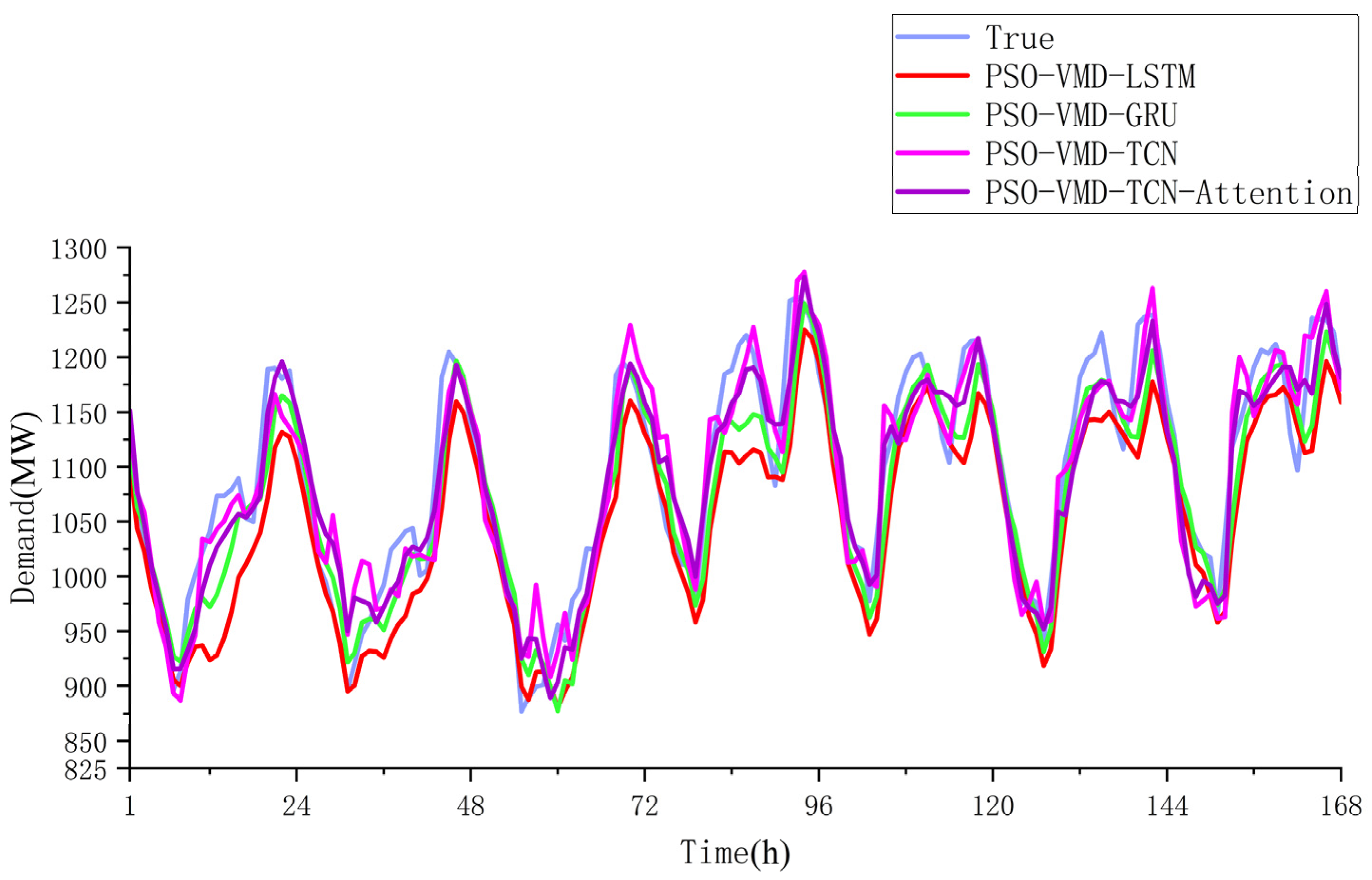
For short-term electricity load forecasting, the evaluation indexes of the TCN-Attention method and the comparison model proposed in this paper are shown in Table 4, and the forecasting results are shown in Figure 7.
Figure 7 displays the prediction result curves of TCN-Attention and the comparison model in short-term power load forecasting. It is apparent from the figure that TCN appropriately captures the nonlinear and non-stationary characteristics of modern power systems, resulting in higher prediction accuracy than LSTM and GRU. Moreover, with the inclusion of the Attention mechanism, TCN accurately forecasts sudden load changes, indicating the mechanism’s ability to assign more significant weight to influential load features, which enhances the model’s prediction accuracy.
Table 4 displays the evaluation results of TCN-Attention and the comparison model for short-term power load forecasting. It is clear from the table that the TCN-Attention model outperforms the comparison model, and it extracts key features more effectively and predicts non-smooth non-linear loads with greater accuracy and efficiency than traditional prediction methods. This solves the issues of challenging feature extraction and low prediction accuracy in existing models.

5. Conclusions

To address the difficulties in extracting modern electric load features and improving prediction accuracy, this paper proposes a method of VMD decomposition based on PSO optimization, which views load sequence decomposition as a critical factor. The short-term electric load prediction framework of PSO-VMD-TCN-Attention is established by combining the TCN prediction model and embedding the Attention mechanism. To verify the effectiveness of PSO-VMD and TCN-Attention, we provide arithmetic examples. The conclusions are presented below.
(1)
By using the VMD decomposition method after PSO optimization to decompose the load, the proposed approach overcomes the need for manual adjustment of parameters required by the VMD decomposition method. The sample entropy is employed as the fitness function for decomposing the load component with the least time complexity, promoting the learning and feature extraction of the forecasting model. The proposed method leads to improved accuracy of the model, as evidenced by the computational analysis.
(2)
The presented example verifies the high prediction accuracy of the TCN-Attention model, which is benefited by several factors: the PSO-optimized VMD’s load sequence construction, TCN’s efficient learning and accurate prediction abilities on load features, and the Attention mechanism’s input sequence weight assignment.
By closely combining the two, the proposed approach resolves the problem of challenging power load feature extraction and enhances the prediction accuracy of the model, ultimately resulting in higher accuracy prediction outcomes.

Author Contributions

Methodology, G.G. and Y.H.; Software, G.G.; Resources, Y.H. and J.Z.; Writing—original draft, G.G.; Writing—review & editing, G.G., Y.H., J.Z., T.Q. and B.Y.; Supervision, Y.H. and J.Z.; Project administration, Y.H.; Funding acquisition, Y.H. and J.Z. All authors have read and agreed to the published version of the manuscript.

Funding

This research was funded by the National Natural Science Foundation of China (NSFC), grant number 51867005, and the Science and Technology Foundation of Guizhou Province, grant numbers ([2022] general013, [2022] general014).

Data Availability Statement

The data is not available to the public.

Conflicts of Interest

The authors declare no conflict of interest.

References

  1. Smil, V. Perils of long-range energy forecasting: Reflections on looking far ahead. Technol. Forecast. Soc. Chang. 2000, 65, 251–264. [Google Scholar] [CrossRef]
  2. Yildiz, B.; Bilbao, J.I.; Sproul, A.B. A review and analysis of regression and machine learning models on commercial building electricity load forecasting. Renew. Sustain. Energy Rev. 2017, 73, 1104–1122. [Google Scholar] [CrossRef]
  3. Zhao, J.; Liu, X.J. A hybrid method of dynamic cooling and heating load forecasting for office buildings based on artificial intelligence and regression analysis. Energy Build. 2018, 174, 293–308. [Google Scholar] [CrossRef]
  4. Ibrahim, B.; Rabelo, L.; Gutierrez-Franco, E.; Clavijo-Buritica, N. Machine Learning for Short-Term Load Forecasting in Smart Grids. Energies 2022, 15, 8079. [Google Scholar] [CrossRef]
  5. Wu, H.; Qi, F.; Zhang, X.; Liu, Y.B.; Xiang, Y.; Liu, J.Y. User-side Net Load Forecasting Based on Wavelet Packet Decomposition and Least Squares Support Vector Machine. Mod. Electr. Power 2023, 40, 192–200. [Google Scholar] [CrossRef]
  6. Tan, Z.; Zhang, J.; He, Y.; Zhang, Y.; Xiong, G.; Liu, Y. Short-Term Load Forecasting Based on Integration of SVR and Stacking. IEEE Access 2020, 8, 227719–227728. [Google Scholar] [CrossRef]
  7. Yang, D.; Yang, J.; Hu, C.; Cui, D.; Cheng, Z.G. Short-term power load forecasting based on improved LSSVM. Electron. Meas. Technol. 2021, 44, 47–53. [Google Scholar] [CrossRef]
  8. Gu, Y.D.; Ma, D.F.; Cheng, H.C. Power Load Forecasting Based on Similar-data Selection and Improved Gradient Boosting Decision Tree. Proc. CSU-EPSA 2019, 31, 64–69. [Google Scholar] [CrossRef]
  9. Wu, X.Y.; He, J.H.; Zhang, P.; Hu, J. Power System Short-term Load Forecasting Based on Improved Random Forest with Grey Relation Projection. Autom. Electr. Power Syst. 2015, 39, 50–55. [Google Scholar]
  10. Li, Y.; Jia, Y.J.; Li, L.; Hao, J.S.; Zhang, X.Y. Short term power load forecasting based on a stochastic forest algorithm. Power Syst. Prot. Control 2020, 48, 117–124. [Google Scholar] [CrossRef]
  11. Cheng, H.X.; Huang, Z. Short-term electric load forecasting model based on improved PSO optimized RNN. Electron. Meas. Technol. 2019, 42, 94–98. [Google Scholar] [CrossRef]
  12. Chen, Z.; Liu, J.; Li, C.; Ji, X.; Li, D.; Huang, Y.; Di, F. Ultra Short-term Power Load Forecasting Based on Combined LSTM-XGBoost Model. Power Syst. Technol. 2020, 44, 614–620. [Google Scholar] [CrossRef]
  13. Peng, W.; Wang, J.R.; Yin, S.Q. Short-term Load Forecasting Model Based on Attention-LSTM in Electricity Market. Power Syst. Technol. 2019, 43, 1745–1751. [Google Scholar] [CrossRef]
  14. Li, P.; He, S.; Han, P.F.; Zheng, M.M.; Huang, M.; Sun, J. Short-Term Load Forecasting of Smart Grid Based on Long-Short-Term Memory Recurrent Neural Networks in Condition of Real-Time Electricity Price. Power Syst. Technol. 2018, 42, 4045–4052. [Google Scholar] [CrossRef]
  15. Yang, L.; Wu, H.B.; Ding, M.; Bi, R. Short-term Load Forecasting in Renewable Energy Grid Based on Bi-directional Long Short-term Memory Network Considering Feature Selection. Autom. Electr. Power Syst. 2021, 45, 166–173. [Google Scholar]
  16. Wang, Z.P.; Zhao, B.; Ji, W.J.; Gao, X.; Li, X. Short-term Load Forecasting Method Based on GRU-NN. Autom. Electr. Power Syst. 2019, 43, 53–58. [Google Scholar]
  17. Xie, Q.; Dong, L.H.; She, X.Y. Short-term electricity price forecasting based on Attention-GRU. Power Syst. Prot. Control 2020, 48, 154–160. [Google Scholar] [CrossRef]
  18. Niu, D.X.; Ma, T.N.; Wang, H.C.; Liu, H.F.; Huang, Y.L. Short-Term Load Forecasting of Electric Vehicle Charging Station Based on KPCA and CNN Parameters Optimized by NSGA II. Electr. Power Constr. 2017, 38, 85–92. [Google Scholar]
  19. Kong, X.Y.; Zheng, F.; Cao, J.; Wang, X. Short-term Load Forecasting Based on Deep Belief Network. Autom. Electr. Power Syst. 2018, 42, 133–139. [Google Scholar]
  20. Liao, N.H.; Hu, Z.Y.; Ma, Y.Y.; Lu, W.Y. Review of the short-term load forecasting methods of electric power system. Power Syst. Prot. Control 2011, 39, 147–152. [Google Scholar]
  21. Ahmad, N.; Ghadi, Y.; Adnan, M.; Ali, M. Load Forecasting Techniques for Power System: Research Challenges and Survey. IEEE Access 2022, 10, 71054–71090. [Google Scholar] [CrossRef]
  22. Ye, J.H.; Cao, J.; Yang, L.; Luo, F.Z. Ultra Short-term Load Forecasting of User Level Integrated Energy System Based on Variational Mode Decomposition and Multi-model Fusion. Power Syst. Technol. 2022, 46, 2610–2618. [Google Scholar] [CrossRef]
  23. Wu, S.M.; Jiang, J.D.; Yan, Y.H.; Bao, W. Short-term Load Forecasting Based on VMD-PSO-MKELM Method. Proc. CSU-EPSA 2022, 34, 18–25. [Google Scholar] [CrossRef]
  24. Liu, K.Z.; Ruan, J.X.; Zhao, X.P.; Liu, G. Short-term Load Forecasting Method Based on Sparrow Search Optimized Attention-GRU. Proc. CSU-EPSA 2022, 34, 99–106. [Google Scholar] [CrossRef]
  25. Yu, J.Q.; Nie, J.K.; Zhang, A.J.; Hou, X.Y. ARIMA-GRU Short-term Power Load Forecasting Based on Feature Mining. Proc. CSU-EPSA 2022, 34, 91–99. [Google Scholar] [CrossRef]
  26. Huang, S.; Zhang, J.; He, Y.; Fu, X.; Fan, L.; Yao, G.; Wen, Y. Short-Term Load Forecasting Based on the CEEMDAN-Sample Entropy-BPNN-Transformer. Energies 2022, 15, 3659. [Google Scholar] [CrossRef]
  27. Wang, C.; Wang, Y.; Zheng, T.; Dai, Z.M.; Zhang, K.F. Multi-Energy Load Forecasting in Integrated Energy System Based on ResNet-LSTM Network and Attention Mechanism. Trans. China Electrotech. Soc. 2022, 37, 1789–1799. [Google Scholar] [CrossRef]
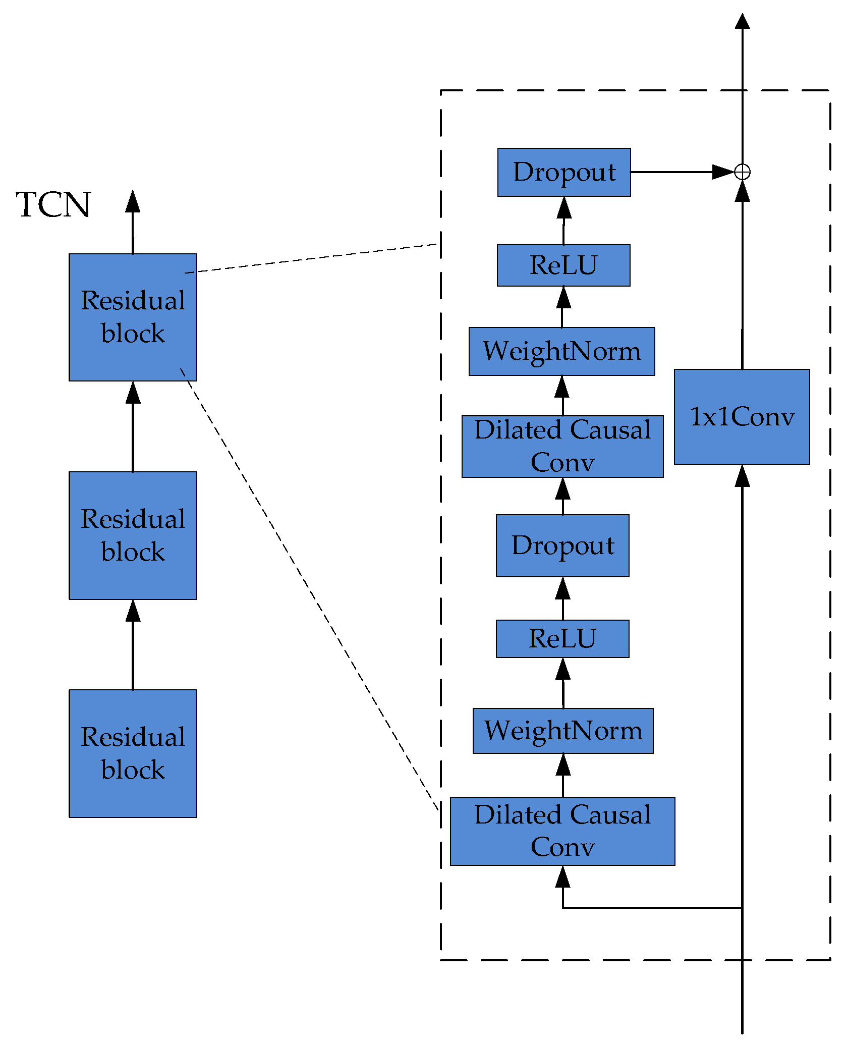
Figure 1. TCN network structure.
Energies 16 04616 g001
Figure 2. Structural diagram of the Attention Mechanism.
Energies 16 04616 g002
Figure 3. Network structure of the TCN-Attention prediction model.
Energies 16 04616 g003
Figure 4. Original power load curve.
Energies 16 04616 g004
Figure 5. VMD component curve.
Energies 16 04616 g005
Figure 6. Comparison of model predictions before and after PSO optimization of the VMD decomposition method.
Energies 16 04616 g006
Figure 7. Comparison chart of model prediction curves.
Energies 16 04616 g007
Table 1. PSO optimized VMD parameter settings.
VMDK (Modal Number)Alpha (Bandwidth Constraint)
Values79800
Table 2. Parameter settings for the TCN-Attention model.
Number of
Neurons N
Activation
Function
Optimization
Algorithm
Training BatchNumber of
Iterations
128ReluAdam64100
Table 3. Comparison of model evaluation indicators before and after PSO optimization.
ModelsRMSEMSEMAEMAPE
LSTM70.7675007.97157.7460.053
GRU75.9505768.43962.5710.057
TCN43.9521931.78732.2670.030
PSO-VMD-LSTM53.9302908.48942.3990.038
PSO-VMD-GRU37.8871435.46229.6280.027
PSO-VMD-TCN35.5971267.15129.2160.027
Table 4. TCN-Attention and comparison model evaluation indicators.
ModelsRMSEMSEMAEMAPE
PSO-VMD-LSTM53.9302908.48942.3990.038
PSO-VMD-GRU37.8871435.46229.6280.027
PSO-VMD-TCN35.5971267.15129.2160.027
PSO-VMD-TCN-Attention33.0791094.23127.4700.025
Disclaimer/Publisher’s Note: The statements, opinions and data contained in all publications are solely those of the individual author(s) and contributor(s) and not of MDPI and/or the editor(s). MDPI and/or the editor(s) disclaim responsibility for any injury to people or property resulting from any ideas, methods, instructions or products referred to in the content.