Fault Recovery Strategy for Power–Communication Coupled Distribution Network Considering Uncertainty

Abstract

In the face of multiple failures caused by extreme disasters, the power and communication sides of the distribution network are interdependent in the fault recovery process. To improve the post-disaster recovery efficiency of the distribution network, this paper proposes a coordinated optimization strategy for distribution network reconfiguration and repair, which integrates the power and communication aspects. First, the recovery process is divided into islanding–reconfiguration and dynamic emergency repair. The coupling relationship between power and communication is considered; that is, power failure may cause communication nodes to lose power, and communication failure may affect the effective operation of remote control devices. Based on this, the fault recovery process is optimized with the objective of maximizing load transfer and direct recovery while introducing a stochastic model predictive control method to handle the uncertainty of distributed power generation by rolling optimization of typical scenarios. Finally, the effectiveness of the proposed strategy is verified using an improved IEEE33-node distribution network system. The simulation results show that the proposed method can recover power to the maximum extent and reduce loss while ensuring the safe and stable operation of the distribution system.

1. Introduction

In recent years, extreme events such as earthquakes and typhoons have occurred frequently [1,2], causing extensive damage to the power system and seriously affecting the safety and stability of the power grid. 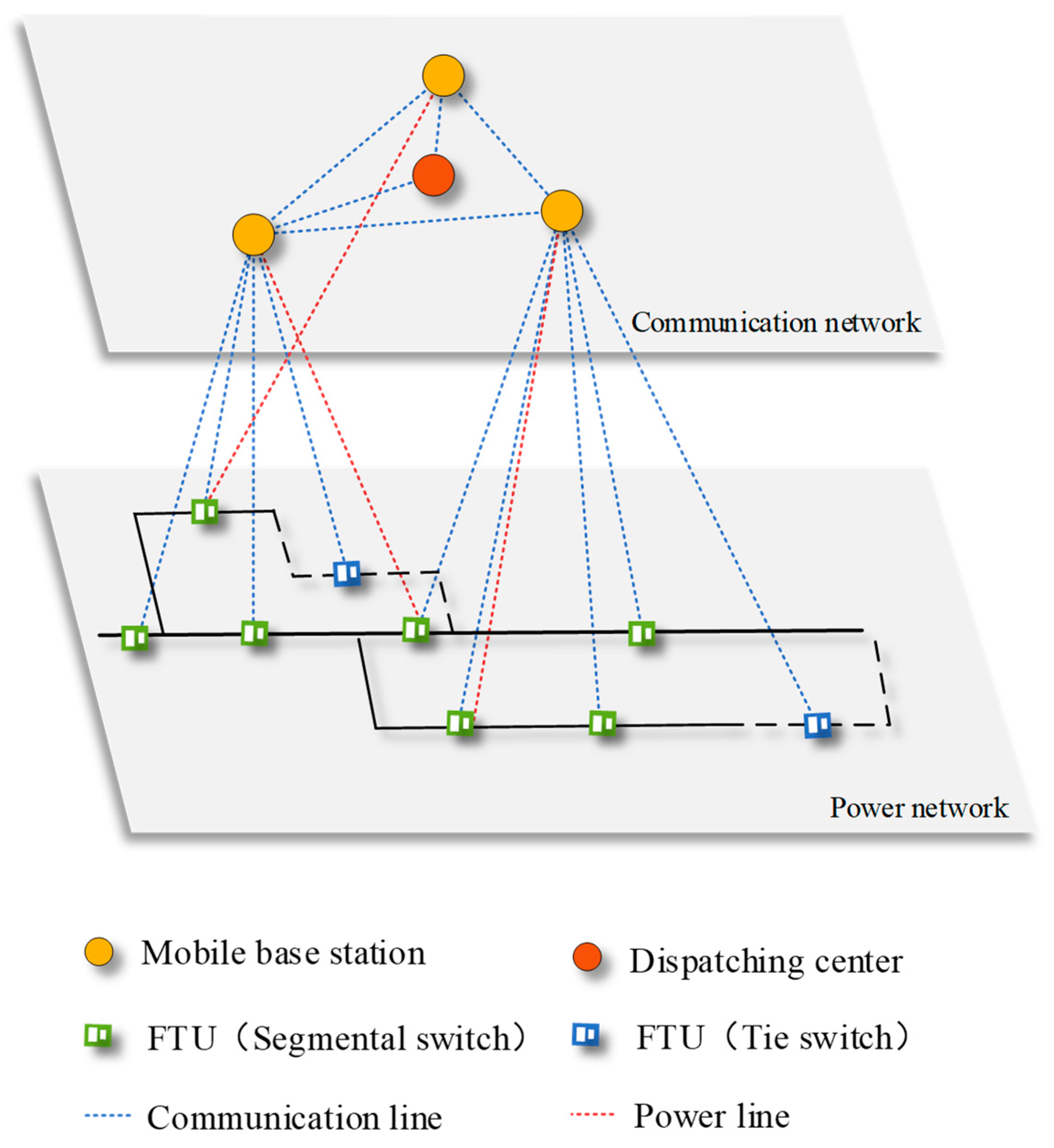At the same time, power and communication devices in the distribution network have formed a strong coupling relationship, which can easily cause the interactive propagation of faults between the two sides of the network [3,4], leading to cascading failures that can cause major power outages. For example, in July 2021, Zhengzhou, Henan province, experienced severe and extreme rainfall, resulting in significant damage to the power system. In total, 736 transformers failed and 6028 power poles collapsed, leading to a large number of base stations being forced out of service due to power outages. According to statistics, a total of 3152 base stations were affected, disrupting the dispatch automation of the power distribution network and triggering a cascade of failures. This led to the shutdown of 473 power distribution lines, impacting approximately 775,000 households’ electricity supply. Due to various factors, including the type and severity of natural disasters, as well as the resilience and disaster resistance capabilities of the equipment, it is difficult to determine which type of failure is more likely to occur. During natural disasters, power failures result in the loss of power to communication equipment, and communication disruptions, in turn, impact the information retrieval and effective operation of remote control devices. Therefore, coordinating the recovery of both power and communication can enhance the distribution network’s ability to respond to disasters.

Many strategies have been proposed for distribution network fault recovery, which utilizes various resources to flexibly reconfigure the network and reduce power outages and economic loss. Ref. [5] proposes a global dynamic reconfiguration method applicable to multi-stage switching modes, which enhances large-scale load flow regulation capability. Ref. [6] considers the capacitor placement problem during distribution network reconfiguration and solves the established mixed-integer linear programming model using CPLEX, effectively reducing node voltage deviations and power loss. Ref. [7] considers the scale and location of distributed generation (DG) in distribution network reconfiguration. It uses a water cycle algorithm based on a discrete search space to significantly improve the operational efficiency of the distribution network. Refs. [8,9] proposes a new radial constraint formula, making distribution network reconfiguration and operation more flexible and enhancing system resilience. However, the above studies do not involve fault repair.

In the recovery process, failure to adjust the network structure after repairing a fault can affect the reliability of the power supply in the distribution network. Reliability is crucial for maintaining system stability, and extensive research has been conducted to explore reliability issues [10,11,12]. Ref. [13] establishes a multi-stage dynamic recovery model based on traffic and energy networks. It deploys mobile energy storage devices to recover power outages based on rapid reconfiguration, achieving coordination and cooperation of various resources during recovery. Ref. [14] proposes a coordinated optimization strategy for distribution network fault reconfiguration and repair with distributed generation, considering the time-varying nature of the load and using an improved particle swarm algorithm for a solution. Ref. [15] proposes a coordinated optimization strategy for distribution network recovery, maintenance personnel, and mobile power dispatch, which is transformed into a mixed-integer linear programming problem. The computational complexity is reduced through preprocessing, improving system resilience. The above studies focus only on the power grid and do not consider the impact of communication failures on distribution network recovery. The actual distribution network recovery process depends on the automated scheduling of communication systems for the power fault location, isolation, and switch action [16,17], while the communication system also depends on a continuous and stable power supply from the power side to maintain normal operation [18,19]. The power and communication sides constrain each other during the distribution network fault recovery process. Therefore, coordination between the two can make the distribution network more efficient and faster to recover, thereby reducing economic loss caused by faults.

Currently, few studies consider the interaction between power and communication in distribution network fault recovery. Ref. [20] proposed a fault correlation matrix that reflects the impact of communication failures on the power side. It established a communication-power bi-level optimization model with coupled constraints prioritizing communication recovery. The model was solved using second-order cone relaxation and dynamic routing algorithms. Ref. [21] quantified the elasticity of distribution networks based on a compound Poisson process, established an optimization model with a cascading failure model, and used an improved simulated annealing algorithm to obtain the optimal repair sequence. Ref. [22] established a unified repair personnel scheduling and time model based on integrating transportation, communication, and power networks. It converted it into a mixed-integer linear programming problem using an improved single-commodity flow model. These studies did not consider the uncertainty of distributed generation output during fault recovery, which makes it difficult to obtain the optimal control sequence, thereby affecting the stable operation of the distribution network and causing additional economic loss.

To address the issues mentioned above, this paper proposes a fault recovery strategy for power–communication coupled distribution network with consideration of uncertainty. Firstly, the recovery process is divided into two stages: islanding–reconfiguration and dynamic emergency repair. The joint optimization of power and communication networks is realized by establishing coupling constraints. Secondly, stochastic model predictive control (SMPC) is used to replace a single prediction sequence with a set of scenarios representing different states for rolling optimization to solve the uncertainty of distributed generation output [23]. Finally, the effectiveness of the proposed method is verified by using the improved IEEE 33-node distribution system.

2. Problem Overview

2.1. The Coupling Mechanism between Power and Communication

The distribution system can be divided into the power side and the communication side. The power side includes nodes, lines, distributed generation, loads, segmental switches, tie switches, etc. In this paper, wireless communication is used. The communication side includes dispatching centers, mobile base stations, and feeder terminal units (FTUs) [24]. FTUs are located at the power node and control the switches between the power node and the upstream node. FTUs and dispatching centers have standby power generation units, which can maintain normal operation even if the power side is out of service. The power–communication coupling is reflected in the fact that the mobile base station depends on the power supply on the power side, and the control of distribution device, such as switches, also depends on control instructions from the communication side. FTUs send operational data of distribution device to the dispatching center via the mobile base station. The dispatching center sends control instructions to FTUs to control the opening and closing of segmental (tie) switches. The system structure is shown in Figure 1.

During the post-disaster recovery process of the distribution network, the impact of the power side on the communication side is mainly reflected in the disconnection of communication nodes due to power failure after the fault, and the degree of impact of the communication side on the power side depends on the role of communication functions in the distribution network fault recovery process. Specifically, the types of communication system failures can be divided into FTU information monitoring device failures and wireless communication network transmission failures [25]. This paper analyzes the impact of communication on the fault recovery of the distribution network from two aspects.

• FTU information monitoring device failure

The information monitoring device collects real-time acquisition of the distribution network’s switch status and power parameters [26]. When a failure occurs, it indirectly affects the dispatch center’s judgment of the fault location [27], further expanding the power outage area. Figure 2 shows the fault state analysis of the distribution network, where a fault occurs between power nodes 3 and 4, and the segmental switch in this section is disconnected because the FTU in this section cannot obtain measurement information. Although no fault occurs between nodes 2 and 3, due to the failure of the FTU information monitoring device, the dispatch center identifies a fault in this section and locates it between nodes 2 and 4. Therefore, the segmental switch between nodes 2 and 3 is disconnected, causing a power outage at node 3 and expanding the power outage area.

• Wireless communication network transmission failure

The dispatch center cannot obtain complete measurement information, and it is difficult to issue relevant control instructions based on the fault situation. This can lead to some switches not operating normally, affecting fault reconfiguration and load transfer, causing more power outages and longer fault recovery time.

2.2. Fault Recovery Strategy Framework

With the increasing integration of DG into distribution networks, it is difficult to obtain the optimal recovery strategy by optimizing based on deterministic power output. This paper proposes the use of SMPC for fault recovery to reduce the impact of renewable energy output uncertainty. The operating principles are shown in Figure 3 as follows.

• At the current time step, denoted as k, the prediction model is used to obtain the wind and solar power prediction sequence for the prediction/optimization horizon;
• The probability distribution of wind and solar power output is usually continuous. Therefore, it is approximated using a finite number of discrete deterministic samples. This paper employs Latin hypercube sampling (LHS) and probability distance reduction (PDR) to generate and reduce the “scenario,” obtaining typical wind and solar power output sequences and their corresponding probabilities [28,29];
• The optimization model consists of islanding–reconfiguration and dynamic repair. Each scenario is incorporated into the optimization model, with the objective function consisting of the loss of load, network loss, social and economic loss, repair cost, etc. The constraints include the power–communication coupling constraint, power flow constraint, node voltage constraint, radial topology constraint, repair resource constraint, etc. The optimization problem is then solved to obtain control sequences for opening and closing switches and repair order for the optimization period. Only the first control variable sequence is issued;
• In the next time step, i.e., the k + 1 time step, the actual measured values of wind and solar power are used as the initial values for the k + 1 time step, thus achieving feedback correction of the prediction model. Then, the process is repeated from step 1 for the next horizon optimization.

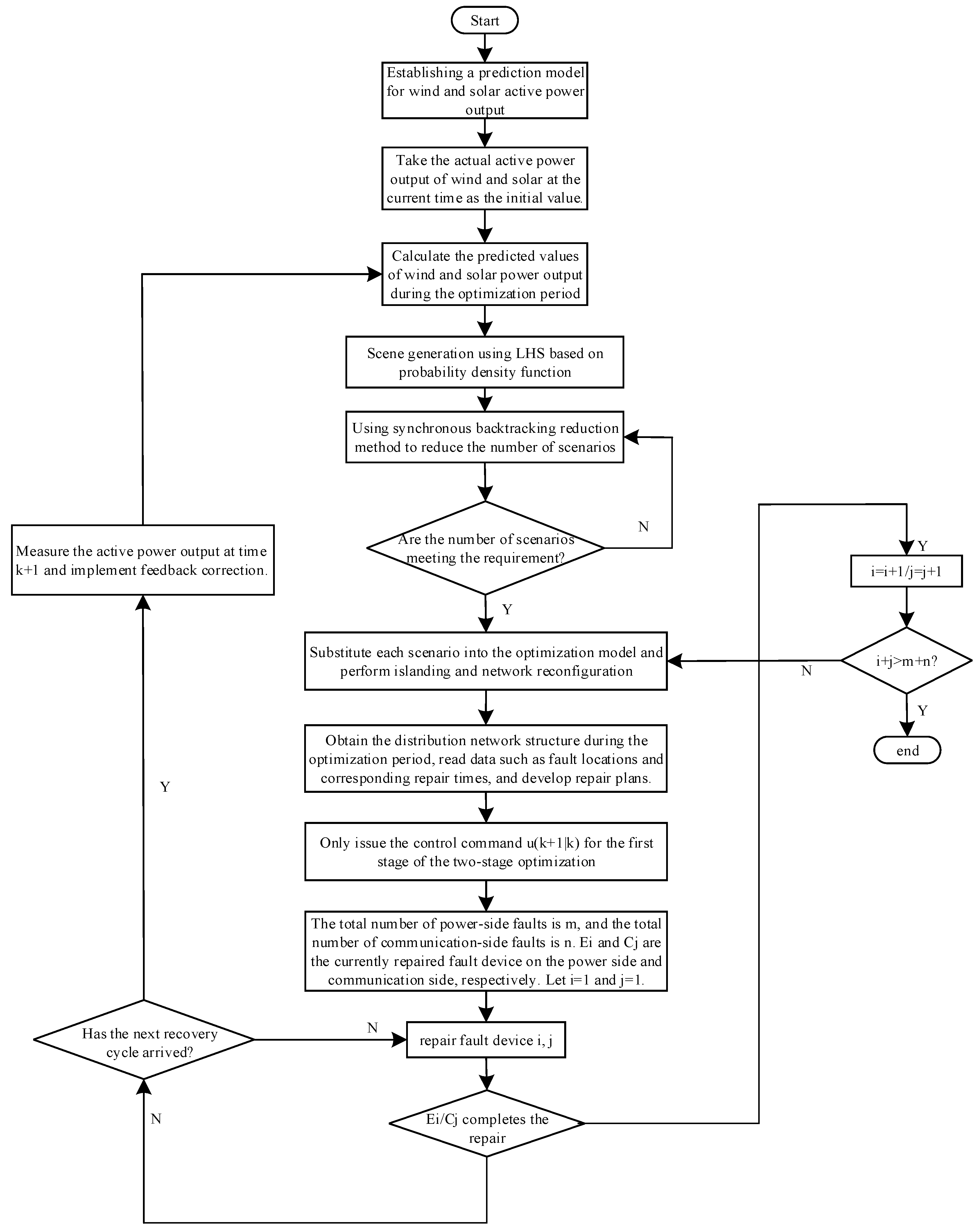
3. Fault Recovery Optimization Model

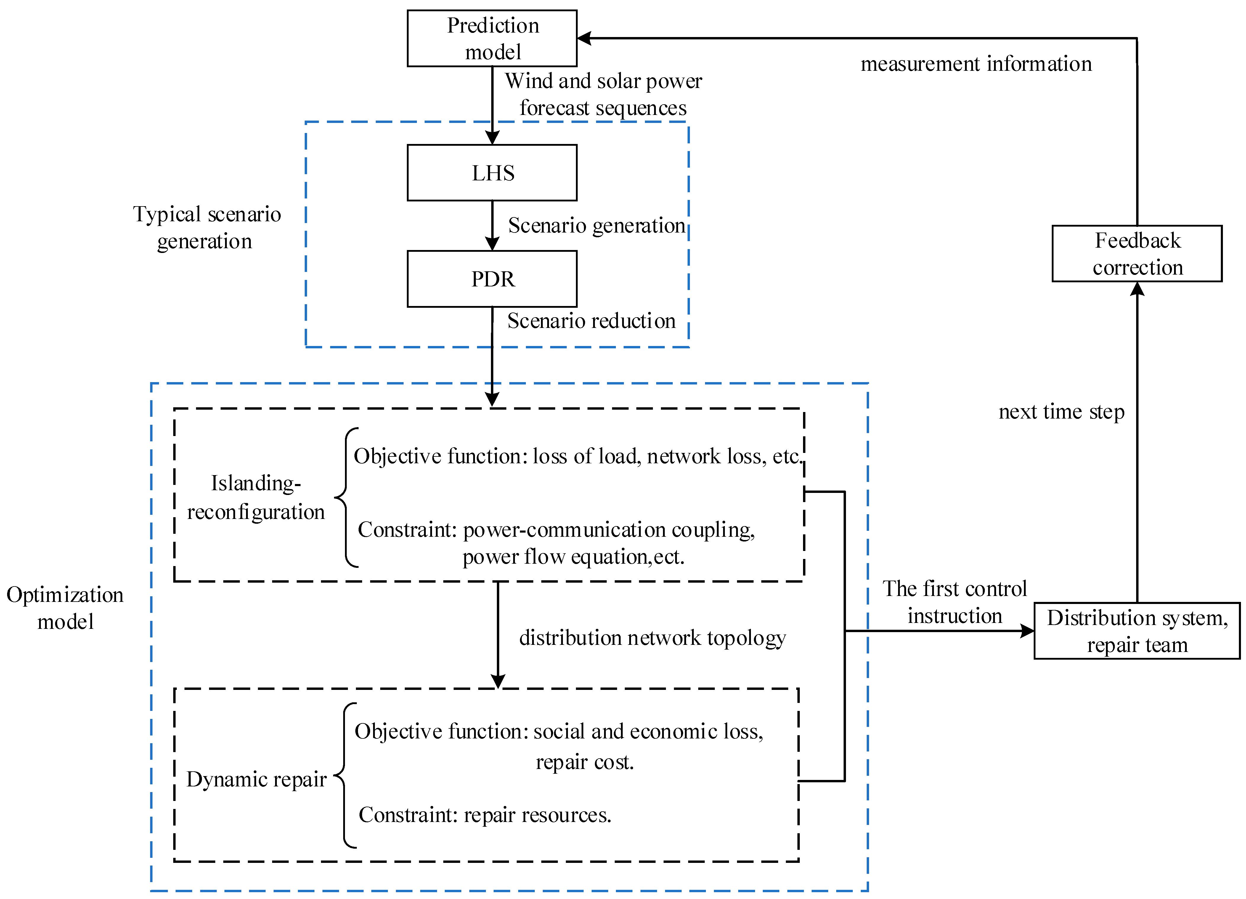
The optimization model is divided into two parts: islanding–reconfiguration and dynamic repair. After optimization, the control sequences for opening/closing and repair order within the optimization period can be obtained. In order to minimize prediction errors as much as possible, repeated rolling optimization is used instead of a one-time global optimization, and only the first control variable sequence is issued.

3.1. Part 1

Part 1 is islanding–reconfiguration. This part considers the impact of communication failures on the normal operation of segmental and tie switches, achieving load transfer and grid reconfiguration. Firstly, islanding is achieved using a topological search method based on the DG load transfer capability. Then, mathematical programming is used to solve the network reconfiguration of the distribution network.

3.1.1. Objective Function

Optimization is carried out for typical scenarios based on comprehensive consideration of factors such as loss of load, node voltage deviation, and network loss.

$$F=\min {\displaystyle \sum _{s=1}^N{p}_s(u_1{f}_1^s+u_2{f}_2^s+u_3{f}_3^s)}$$

(1)

where p_s represents the probability of the s-th scenario; u₁, u₂, and u₃ are the weight values of the loss of load, node voltage deviation, and network loss in the objective function, respectively; $f_1^s$, $f_2^s$, and $f_3^s$ are the total loss of load, node voltage deviation, and network loss in the s-th scenario; and N is the number of typical scenarios.

• Loss of load

$$f_1=\min {\displaystyle \sum _{i=1}^M{\omega }_i{P}_i^{cut}}$$

(2)

where ω_i represents the load level coefficient of node i, with values of 100, 10, and 1 for the first, second, and third level loads, respectively; M is the total number of blackout load nodes; and $P_i^{cut}$ is the load power cut off at node i.

• Node voltage deviation

The node voltage deviation can measure the degree of voltage offset, and a smaller deviation indicates less voltage fluctuation in the distribution network, resulting in higher power supply reliability.

$$f_2=\min {\displaystyle \sum _{k=1}^N\left(\left|U_k-U_s\right|/U_s\right)}$$

(3)

where N represents the total number of main network nodes in the distribution network; U_k represents the voltage value at node k; and U_s represents the reference voltage value of the distribution network.

• Network loss

$$f_3=\min {\displaystyle \sum _{j\in L}{k}_j{r}_j}\left(P_j^2+Q_j^2\right)/U_j^2$$

(4)

where L represents the set of branches in the distribution network and k_j represents the current status of the segmental switch on branch j. If it is closed, then k_j equals 1; otherwise, k_j equals 0. P_j, Q_j, and U_j, respectively, represent the current active power, reactive power, and voltage magnitude of branch j. r_j represents the resistance of branch j.

3.1.2. Constraints

• Power–communication coupling constraint

The power and communication sides mutually influence each other during the recovery process, which results in segmental (tie) switch state constraint and power supply constraint.

$$k_{x\left(y\right)}\le k\begin{array}{cc}{}_{x\left(y\right)}^c& x\in {\Omega }_a,\end{array}y\in {\Omega }_b$$

(5)

$$C_i=D_i^1\cup D_i^2\cdots \cup D_i^M$$

(6)

where k_x(y) represents the status of the segmental switch x (tie switch y), and $k_{x\left(y\right)}^c$ represents whether communication failure has affected the normal operation of the segmental switch x (tie switch y). When $k_{x\left(y\right)}^c$ equals 1, there is no impact, and when it equals 0, there is an impact. Ω_a and Ω_b represent the set of segmental switches and tie switches, respectively. C_i represents the communication node i, and $D_i^M$ represents the power node corresponding to the Mth power supply demand of the communication node i.

• Power flow constraint

$$\left\{\begin{array}{l}{U}_i-U_j=Z_{ij}{I}_{ij}\\ S_{ij}=U_i{I}_{ij}^{\ast }\\ {\displaystyle {\sum }_{a:a\to i} s_i+(S_{ai}-Z_{aj}{\left|I_{ai}\right|}^2)={\displaystyle {\sum }_{j:i\to j} }{S}_{ij}}\end{array}\right.$$

(7)

where U_i and U_j represent the voltage of node i and node j, and S_ij and I_ij represent the apparent power and current of the branch from node i to node j, respectively. S_ai, Z_ai, and I_ai represent the apparent power, impedance, and current of the branch from node k to node i, and s_i represents the power capacity access in node i.

The process of transforming the power flow constraints from a nonlinear programming model to a second-order cone programming model using second-order cone relaxation is not described in detail here [30].

• Node voltage constraint

$$U_{\min }\le U_i\le U_{\max }$$

(8)

where U_i represents the voltage value at node i; and U_min and U_max represent the minimum and maximum voltage values allowed at the node.

• Branch current constraint

$$I_l\le I_{l\max }$$

(9)

where I_l is the current flowing through branch l, and I_lmax is the maximum allowed current on branch l.

• Radial topology constraint

In order to reduce power losses and improve power supply reliability, the configuration of distribution networks is typically designed in a radial pattern, which means there are no loops.

$$\left\{\begin{array}{l}{\displaystyle \sum _{l\in \theta }{k}_l}=n_s-n_b\\ k_l\in \left\{0,\left.1\right\}\right.,\forall l\in \theta \end{array}\right.$$

(10)

where k_l represents the binary nominal variable for the switching state of branch l: where it equals 0, this indicates the branch is open, and where it equals 1, this indicates the branch is closed. θ represents the set of distribution network lines; and n_s and n_b represent the total number of nodes and the number of root nodes in the distribution network, respectively.

3.2. Part 2

Part 2 is dynamic recovery, in which the distribution network structure may change after each islanding and network reconfiguration, and power and communication failures can be directly or indirectly recovered to achieve load transfer. Therefore, considering the social and economic loss and repair costs comprehensively, the recovery effect is quantified, and the repair order is dynamically adjusted during recovery.

3.2.1. Objective Function

Based on the consideration of factors such as social and economic loss and repair cost, optimization and solution are conducted based on the known structure of the current distribution network.

$$G=\min ({\lambda }_1{g}_1(X)+{\lambda }_2{g}_2(X))$$

(11)

where X = (x₁, x₂,…, x_n) represents the repair strategy for the faulty device, and n is the total number of faulty devices. λ₁ and λ₂ are the weight values of social and economic loss and repair costs, respectively. g₁(X) and g₂(X) represent the current repair strategy’s social and economic loss and repair costs.

• Social and economic loss

Social and economic loss involves the loss of load and the time required for fault repair at each recovery stage. Therefore, optimizing social and economic loss is beneficial for supplying power to as many users as possible, reducing the impact of faults, and enhancing the reliability of the distribution network.

$$g_1(X)=\min {\displaystyle \sum _{i=1}^n(T(x_i)}-T(x_{i-1})){\displaystyle \sum _{j=1}^3{\omega }_j{P}_j^{scut}(x_i)}$$

(12)

where T(x_i) represents the time when the faulty device x_i is repaired, and $P_j^{scut}\left(x_i\right)$ represents the total power loss of load level j when repairing the faulty device x_i.

• Repair cost

$$g_2(X)=\min \left\{\left.mg+[T_{}(x_{end}^e)+T_{}(x_{end}^c)-2T_{}(x_0)](r+v/l)\right\}\right.$$

(13)

where mg is the fixed cost for repairing the faulty device. $T\left(x_{end}^e\right)$ and $T\left(x_{end}^c\right)$ are the time when the last fault is repaired by the power repair team and the communication repair team, respectively. T(x₀) is the starting time of the repair. r, v, and l represent the labor cost per unit time of each repair team, the driving speed of the repair vehicle, and the unit travel cost, respectively.

3.2.2. Constraints

• Repair device constraint

Power and communication faults can be repaired only by corresponding types of repair teams, and each repair team can repair only one faulty device at a time.

$$\left\{\begin{array}{l}{\displaystyle \sum _{i=1}^{ne}{C}_i^{re}=1}\\ {\displaystyle \sum _{j=1}^{n\mathrm{c}}{C}_j^{rc}=1}\end{array}\right.$$

(14)

where ne represents the number of power system faults, and nc represents the number of communication faults. $C_i^e$ and $C_j^c$, respectively, indicate whether power device i and communication device j are being repaired by the power repair team re and communication repair team rc at the current time. A value of 1 indicates that they are being repaired, while 0 indicates that they have not been repaired yet.

• Repair time constraint

Regardless of the type of fault, it is considered completely recovered after one repair, and there is no need for further repairs.

$${\displaystyle \sum _{i=1}^n{D}_k\left(x_i\right)=1, }\begin{array}{c}k\in {\Omega }_r\end{array}$$

(15)

where k represents the faulty device; Ω_r represents the set of power and communication faulty devices; D_k(x_i) indicates whether the repair order of the faulty device k is the i-th: if yes, then D_k(x_i) = 1, otherwise D_k(x_i) = 0.

4. Fault Recovery Strategy Based on SMPC

The actual output of DG may deviate from the predicted value. If the deterministic output is used for optimization [31], obtaining the optimal control sequence is difficult, and it may affect the power balance of the distribution network. This paper uses the SMPC approach to implement the recovery of the power–communication coupled network under uncertainties caused by renewable energy sources.

4.1. Prediction Model

Renewable energy sources such as wind and solar participate in the flexible operation of the distribution network by increasing or decreasing their power output. Therefore, the changes in the power output of wind and solar power are used as the control variables, and the prediction model is shown below [32]:

$$P\left(k+i | k\right)=P_0\left(k\right)+{\displaystyle \sum _{t=1}^i\Delta u\left(k+t | k\right)} i=1,2,\cdots ,N$$

(16)

where P₀(k) represents the initial output value of renewable energy sources, that is, the actual output value, N is the number of prediction steps, and ∆u(k + t|k) represents the prediction of the change in renewable energy output from [k + t−1, k + t] time interval at time k. P₀(k + i|k) represents the predicted value of renewable energy output at k + i time.

4.2. Typical Scenario Generation

Wind and solar power are renewable energy sources, and their power output is uncertain. Considering the probability distribution function of the power output, many wind and solar scenarios are obtained using Latin hypercube sampling. However, too many samples will lead to overly complex calculations. Therefore, the probability distance reduction method is used to reduce the number of scenarios while ensuring the accuracy of the sample fitting.

4.2.1. Scenario Generation

LHS divides the cumulative density function into m equal regions and randomly samples from each region, achieving nearly all possible scenarios in the sampling results [33]. Compared with Monte Carlo sampling, it has the advantages of comprehensive sampling and no obvious clustering. If there are n variables and m samples need to be drawn from a specified interval, the specific steps of LHS are as follows:

• Divide the cumulative distribution function of each variable into m regions;
• Randomly sample m regions from the n variables, with a total of n × m samplings;
• Randomly combine the N values randomly selected from each variable with the values of other variables.

4.2.2. Scenario Reduction

The optimization solution will become too complex when there are too many scenarios. To balance computation accuracy and time, a synchronous backtracking reduction method based on probability distance is used to reduce the number of scenarios. This method ensures that the wind and solar power output sample set after reduction can better reflect the distribution of random variables while preserving boundary samples and covering various extreme cases. The basic idea is as follows:

• Compute the geometric distance between each pair of scenarios in the scenario sample set.

  $$d_{ij}=\sqrt{{{\displaystyle \sum _{t=1}^n\left(x_i\left(t\right)-x_j\left(t\right)\right)}}^2}, x_i,x_j\in S$$

  (17)

  where S represents the set of scenarios, x_i and x_j, respectively, represent the i-th and j-th scenarios, x_i(t) represents the data corresponding to the t-th dimension in the scenario i, and d_ij represents the distance between scenarios i and j.
• Find the scenario x_k with the closest distance to x_i in the scenario set and obtain the corresponding probability distance D_i.

  $$D_i=p_i{d}_{ik}=p_i\min \left(d_{i1},d_{i2},\cdots d_{in}\right)$$

  (18)

  where p_i represents the probability of scenario x_i, d_ik represents the geometric distance between x_i and x_k, and n is the number of scenarios.
• Sort all probability distances D in the scenarios, eliminate the scenario x_i corresponding to the minimum probability distance, and update the probability of the scenario x_k closest to it.

  $$p_k=p_k+p_i$$

  (19)
• Repeat steps 1–3 until the remaining number of scenarios meets the requirements.

4.3. Feedback Correction

Due to the uncertainty of wind and solar power output and environmental factors, the predicted wind and solar power output values by the forecasting model cannot accurately track the actual output values, and prediction errors exist. Therefore, a feedback correction process is introduced to minimize errors [34]. Specifically, the actual current wind and solar power output values are used as the initial values for the new round of rolling optimization.

$$P_0(k+1)=P_{real}(k+1)$$

(20)

where P₀(k + 1) is the initial power output of renewable energy at time k + 1, and P_real(k + 1) represents the actual power output value obtained at time k + 1 through distribution network measurement devices after the control sequence issued by the dispatch center at time k.

The fault recovery flowchart is shown in Figure A1.

5. Example Analysis

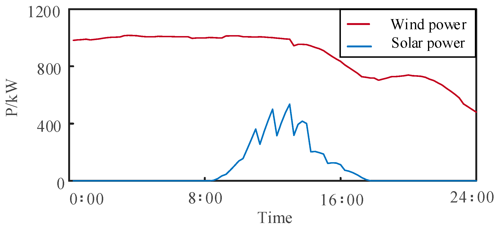
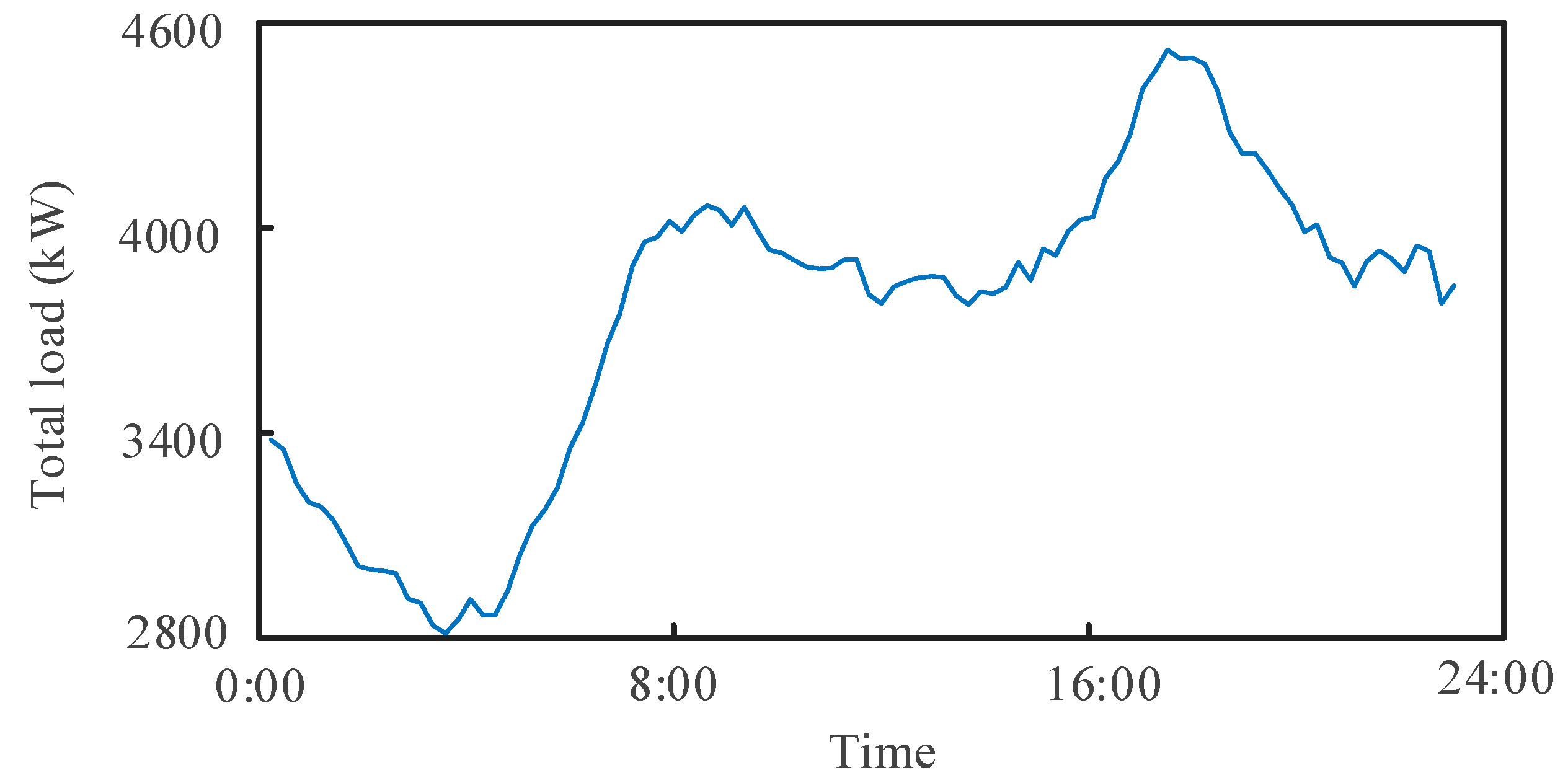
This article uses the IEEE 33-node distribution system for simulation verification, and we adhere to the grid code specified by GB 50052-2009. The grid code provides technical requirements and guidelines for the operation and connection of power systems. The connection points for DG1, DG2, DG3, and DG4 are manually set to nodes 6, 13, 24, and 31, respectively. The maximum power capacities are manually set to 800 kW, 800 kW, 1200 kW, and 1200 kW for DG1, DG2, DG3, and DG4, respectively. DG1 and DG2 are photovoltaic power generation, while DG3 and DG4 are wind power generation. Additionally, it is set that DG1 is restricted to operate within the main distribution network and is unable to form an island independently. The load profile and node load parameters are shown in Appendix Figure A2 and

Table A1. Node load parameters.

Node	Load Class	Node	Load Class	Node	Load Class
0		11	Ⅱ	22	Ⅱ
1	Ⅲ	12	Ⅰ	23	Ⅰ
2	Ⅲ	13	Ⅰ	24	Ⅰ
3	Ⅲ	14	Ⅲ	25	Ⅲ
4	Ⅲ	15	Ⅱ	26	Ⅱ
5	Ⅰ	16	Ⅱ	27	Ⅲ
6	Ⅰ	17	Ⅰ	28	Ⅲ
7	Ⅱ	18	Ⅲ	29	Ⅰ
8	Ⅲ	19	Ⅲ	30	Ⅱ
9	Ⅲ	20	Ⅲ	31	Ⅰ
10	Ⅲ	21	Ⅲ	32	Ⅱ

, respectively. The power line fault is approximately located in the middle of adjacent power nodes. Taking power node “0” as the origin, the power node and communication node coordinates are shown in Appendix

Table A2. Positions of power nodes.

Node	Coordinate/m	Node	Coordinate/m	Node	Coordinate/m
0	(0, 0)	11	(9027, 345)	22	(2621, −2485)
1	(372, −142)	12	(9336, 214)	23	(4062, −2843)
2	(961, −342)	13	(11,532, −348)	24	(4356, −2354)
3	(1549, 42)	14	(11,921, −301)	25	(5734, −1653)
4	(2383, −216)	15	(13,123, 652)	26	(6239, −1647)
5	(3063, 186)	16	(14,235, −1064)	27	(7336, −1364)
6	(4339, 395)	17	(16,682, −1431)	28	(8014, −1112)
7	(5156, 274)	18	(1034, 3140)	29	(8816, −613)
8	(6923, 240)	19	(2632, 2230)	30	(10,353, −924)
9	(7719, 211)	20	(4193, 2843)	31	(10,632, −1023)
10	(8593, −132)	21	(5259, 4023)	32	(11,237, −1356)

and

Table A3. Positions of communication nodes.

Node	Coordinate/m	Node	Coordinate/m
38	(2063, 15)	43	(7227, −1345)
39	(5672, −142)	44	(10,936, 214)
40	(11,961, 142)	45	(6532, −348)
41	(3549, 2942)	46	(7931, 961)
42	(3383, −1216)	47	(6123, −752)

. It is assumed that there is one power repair team and one communication repair team at power node “0”. The fixed repair costs for power and communication faults are 1000 and 2000 yuan, respectively, and the repair time for the faulty device is half an hour. The repair vehicle speed is 60 km per hour, costing 10 yuan per kilometer. The labor cost is 100 yuan per hour, and the recovery starts at 12:00. The rolling optimization interval in this article is 15 min, and the optimization period is 1 h. The number of scenarios generated by LHS is set to 1000, and the reduced typical scenarios number is 5. The CPLEX solver in MATLAB 2018a was used to solve the optimization model.

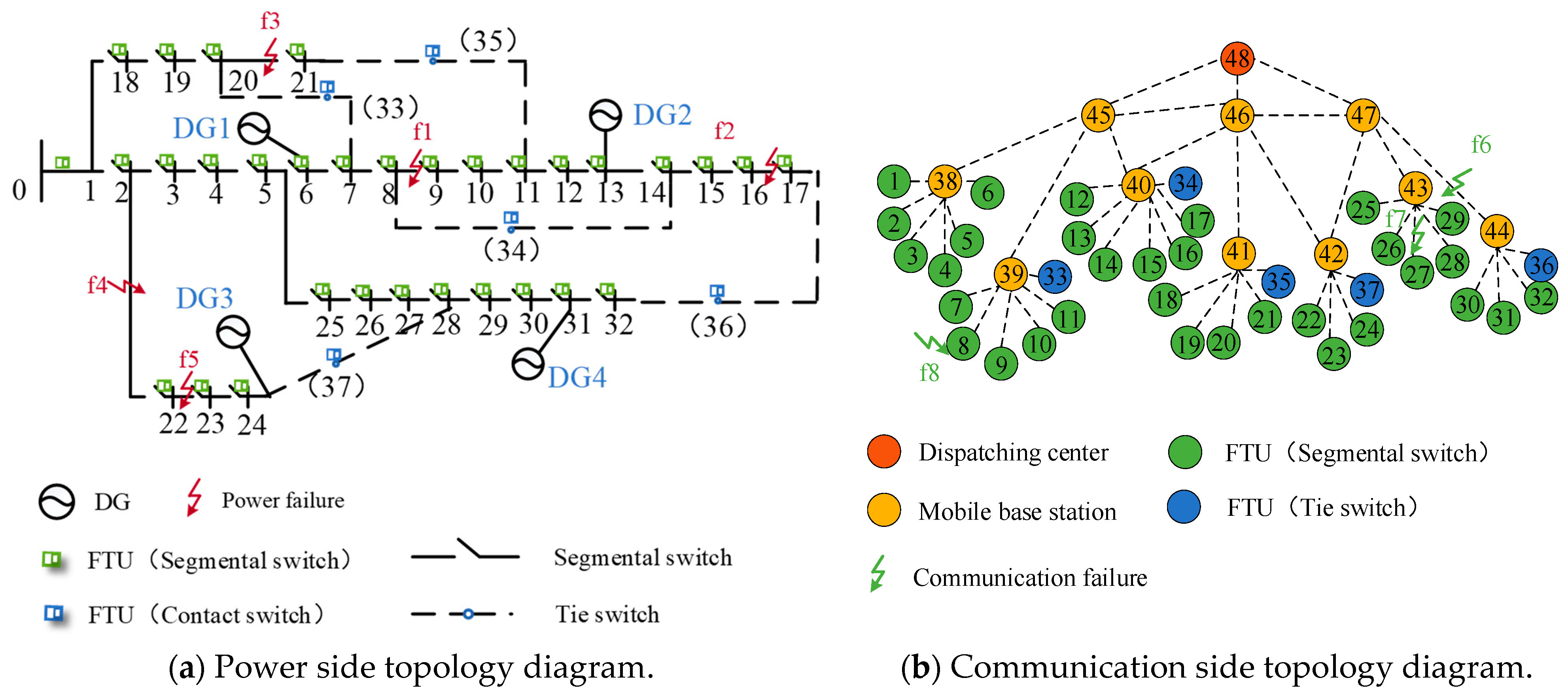
Assuming that there are five power faults and three communication faults in the distribution network, the power faults are located on power lines 8–9, 16–17, 20–21, 2–22, and 22–23, and the communication faults are caused by the failure of wireless transmission on 44–47 due to the communication base station-44 fault, the failure of the control command receiving device on 27–43 caused by the FTU-27 failure, and the location error caused by the information monitoring device failure on FTU-8. The power and communication topology of the distribution network are shown in Figure 4a,b.

Table 1. Coupled network’s power supply relationships.

Communication Node	Power Node	Communication Node	Power Node
38	1, 4	43	25, 27, 28
39	6, 8, 9	44	30, 32
40	12, 14	45	5, 7
41	8, 21	46	3, 5, 23
42	22, 24	47	24, 26

and

Table 2. Coupled network’s control relationships.

Communication Node	Switch
38	1, 2, 3, 4, 5, 6
39	7, 8, 9, 10, 11, 33
40	12, 13, 14, 15, 16, 17, 34
41	18, 19, 20, 21, 35
42	22, 23, 24, 37
43	25, 26, 27, 28, 29
44	30, 31, 32, 36

, respectively, show the coupled network’s power supply and control relationships.

5.1. Simulation Results Analysis

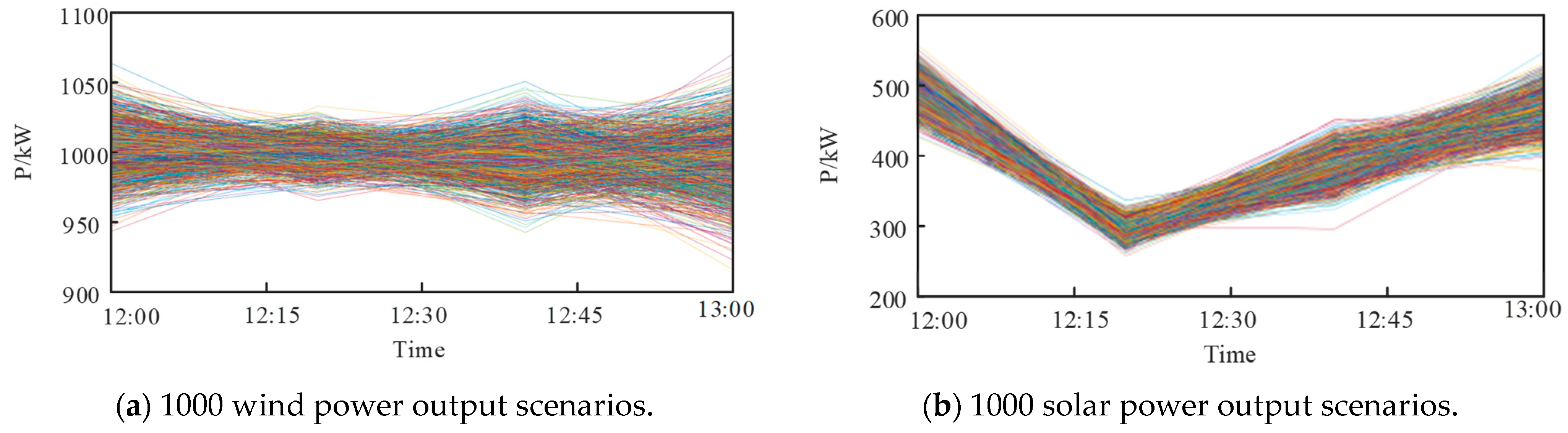
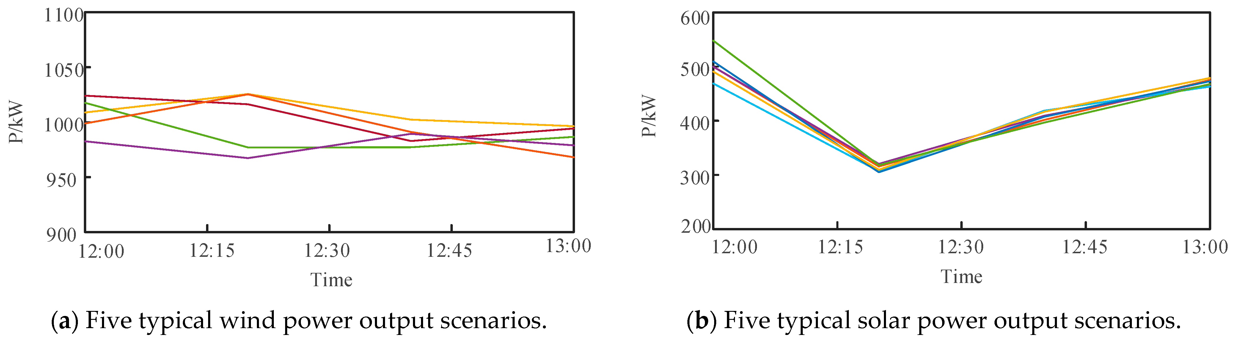
The predicted wind and solar power output on the day of the fault is shown in Figure 5. Figure 6a,b shows 1000 wind and solar power output scenarios generated by LHS in the first optimization period. Figure 7a,b shows five typical wind and solar power output scenarios obtained after scenario reduction in the first optimization period.

Typical wind and solar output scenarios were used to optimize the control sequence for each optimization period. Rolling optimization was used instead of global optimization to minimize prediction errors, and only the first control variable sequence was issued. The device being repaired by the repair team was not included in the optimization of the repair order. Therefore, the focus was on the topology and repair order of the distribution network when the eight faults were repaired. 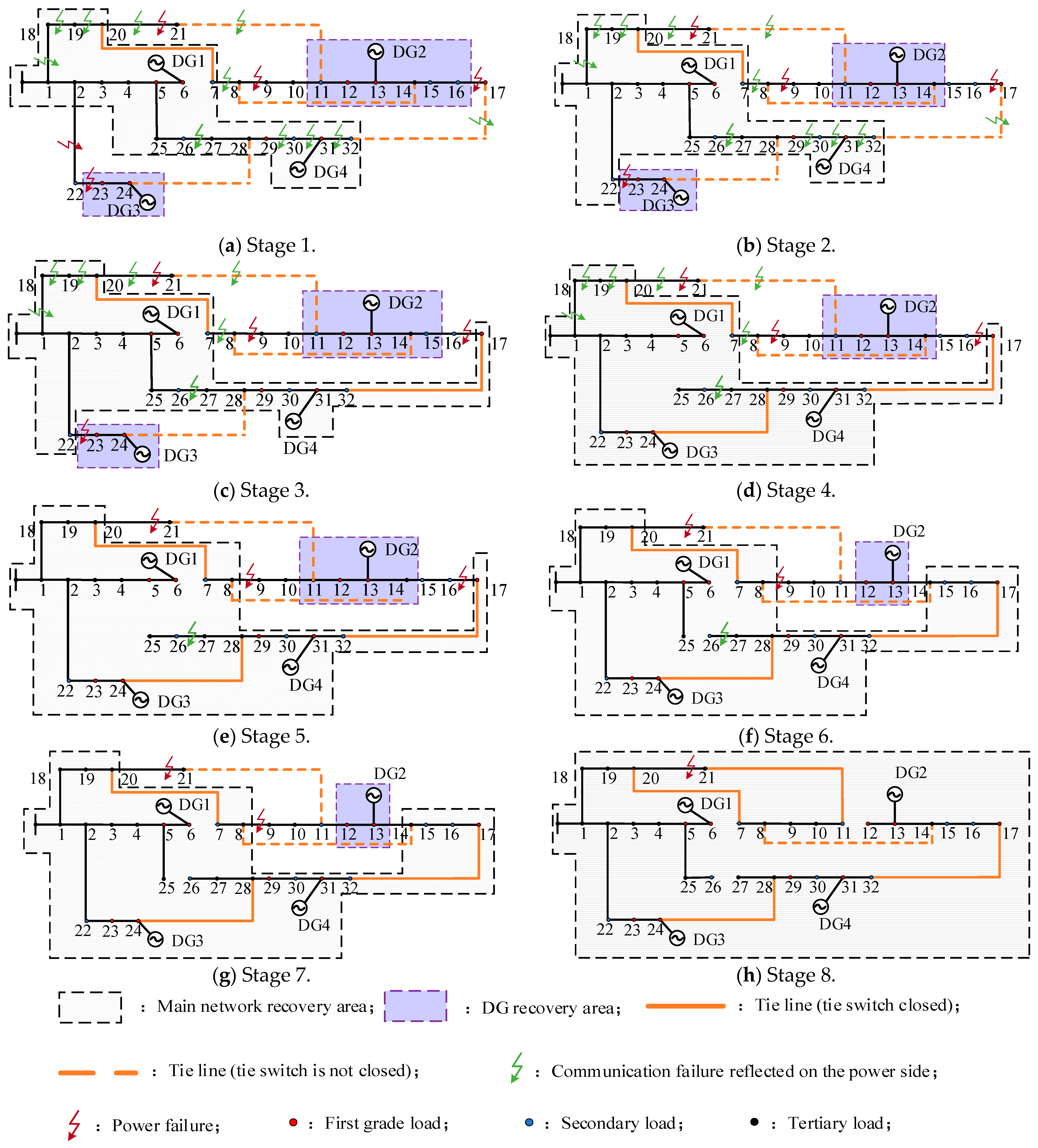Figure 8 shows the topology of the distribution network in each stage of fault recovery, and

Table 3. Repair order.

Stage	Time/min	Devices That Were Repaired	Devices That Were Being Repaired	Power Repair Team Task	Communication Repair Team Task
1	0			f4→f5→f3→f1→f2	f6→f8→f7
2	54.4	f4	f6	f5→f3→f1→f2	f8→f7
3	68.0	f6	f5	f2→f3→f1	f8→f7
4	109.0	f5	f8	f2→f3→f1	f7
5	127.1	f8	f2	f1→f3	f7
6	179.5	f2	f7	f1→f3
7	181.9	f7	f1	f3
8	243.2	f1	f3
9	300.1	f3

shows the repair order in each stage.

As shown in Figure 8 and Table 3, with the repair of faulty devices and the continuous change of DG output, the distribution network topology and the blackout load will also change, and the repair order will be dynamically adjusted. Table 3 shows that the power repair order in stage 3 has changed compared to stage 2. The reason is that when f6 (communication base station-44) is repaired, tie switch-36 can receive the control command from the dispatch center. Before f6 is repaired, f2 was arranged to be repaired last because it is too far from the repair team and takes longer to repair. Additionally, tie switch-36 cannot receive the control command, so it cannot be closed, and repairing f2 first will not recover power to any blackout load. After f6 is repaired, it is predicted that the photovoltaic output will gradually decrease in the next hour, causing secondary load-15 to leave the island. Repairing f2 directly recovers secondary load-16 and indirectly reduces the amount of future blackout load. Repairing f3 and f1 correspond to recovering tertiary load-21 and cannot recover any load, respectively. The disadvantage of repairing f2 is that the overall repair time takes too long, leading to social and economic loss and increased repair cost. The optimal solution in stage 3 corresponds to prioritizing the repair of f2, so the benefits outweigh the drawbacks, and the repair order is changed.

The power repair order in stage 5 has also changed compared to stage 4. When the information monitoring device of FTU-8 is repaired, the measurement information in that section can be transmitted to the dispatch center, so the fault location is reidentified. The dispatch center believes that the power nodes in sections 8 and 9 have not failed and sends instructions to open and close the switch in segments. On the one hand, load-8 is recovered, and the corresponding communication base station-41 also resumes service, so the relevant segmental switch and tie switch can work normally. On the other hand, repairing f1 can recover loads 9 and 10, resulting in a change in the repair order, with f1 being repaired before f3.

5.2. Comparison of Different Control Methods

• Case 1 (deterministic optimization): considering the fluctuation of DG output, but only one optimization was performed using the forecast data for the following day.
• Case 2 (MPC): considering the fluctuation of DG output, reducing the influence of uncertainty, and implementing rolling optimization.
• Case 3 (RMPC): Robust Model Predictive Control (RMPC) based on MPC and robust optimization theory, the modeling of DG output is performed using interval values, further reducing the impact of uncertainty [35].
• Case 4 (SMPC): based on MPC, considering typical scenarios, further reducing the impact of uncertainty.

Case 1 involves a single global optimization without considering the uncertainty of DG output. In Case 2, rolling optimization is used to reduce the impact of uncertainty. Both Case 3 and Case 4 further reduce the DG uncertainty. Comparing the two, Case 3 is better suited for extreme situations but can be overly conservative. On the other hand, Case 4 considers typical scenarios, enabling better adaptation to different situations and providing robust control strategies, although it may have limited capabilities in handling rare or extreme cases.

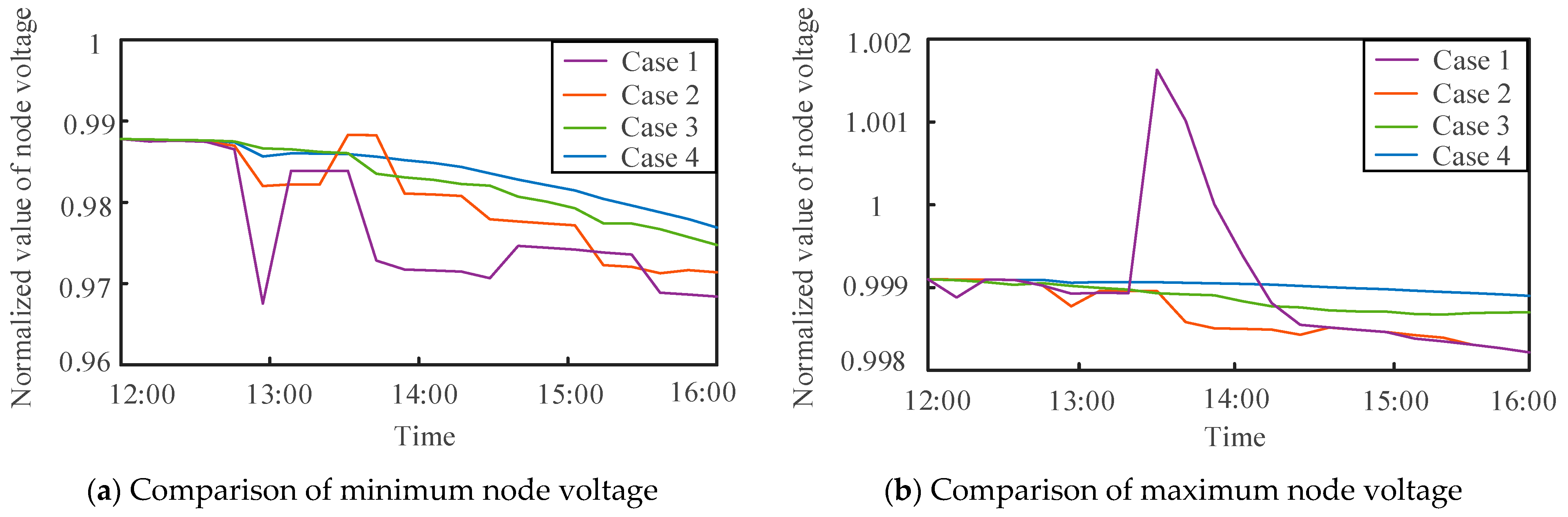
5.2.1. Comparison of Node Voltages

Using the four different control methods to implement fault recovery, and comparing the real-time minimum and maximum node voltage values of the four methods, Figure 9 shows the node voltage values under different control methods.

According to Figure 9, the node voltage deviation is the largest for the method without MPC, because it performs only one global optimization, leading to large errors in the DG power prediction. The MPC method improves the prediction accuracy by considering the fluctuation of DG output and using rolling optimization to obtain the optimal control sequence, resulting in a significant reduction in node voltage deviation. RMPC and SMPC further reduce the impact of uncertainty by utilizing interval modeling and typical scenario approximation, respectively. As a result, the node voltage deviation values are smaller compared to other methods, which is beneficial for the safe and stable operation of the system. Comparing RMPC and SMPC, SMPC generally outperforms RMPC because it can better adapt to different situations, while RMPC tends to be more conservative and shows advantages only in extreme cases.

5.2.2. Comparison of Optimization Results

The results of the four methods are shown in

Table 4. Optimization results.

Method	Social and Economic Loss/kWh	Repair Time/min
Case 1	22,657.4	311.8
Case 2	17,017.3	288.6
Case 3	15,163.1	300.1
Case 4	14,310.5	295.4

. It can be seen from the comparison that the method without MPC has the highest social and economic loss and repair time values, mainly because it only performs one global optimization, and it is difficult to obtain optimal network reconfiguration and repair order instructions. For example, in this case, f2 was repaired as a priority in the third stage, but the method without MPC did not change the repair order, resulting in a delay in the recovery of secondary load-16, causing additional economic loss. MPC, RMPC, and SMPC have the capability of rolling optimization, enabling them to dynamically adjust network architecture and repair order. As a result, these three methods exhibit significant reductions in social and economic loss. Compared to MPC, both RMPC and SMPC demonstrate lower social and economic loss because they further reduce the impact of DG output uncertainty and can potentially recover more power during network reconfiguration by obtaining relatively optimal control sequences. When comparing RMPC and SMPC, SMPC achieves better fault recovery performance due to its superior adaptability.

5.3. Sensitivity Analysis

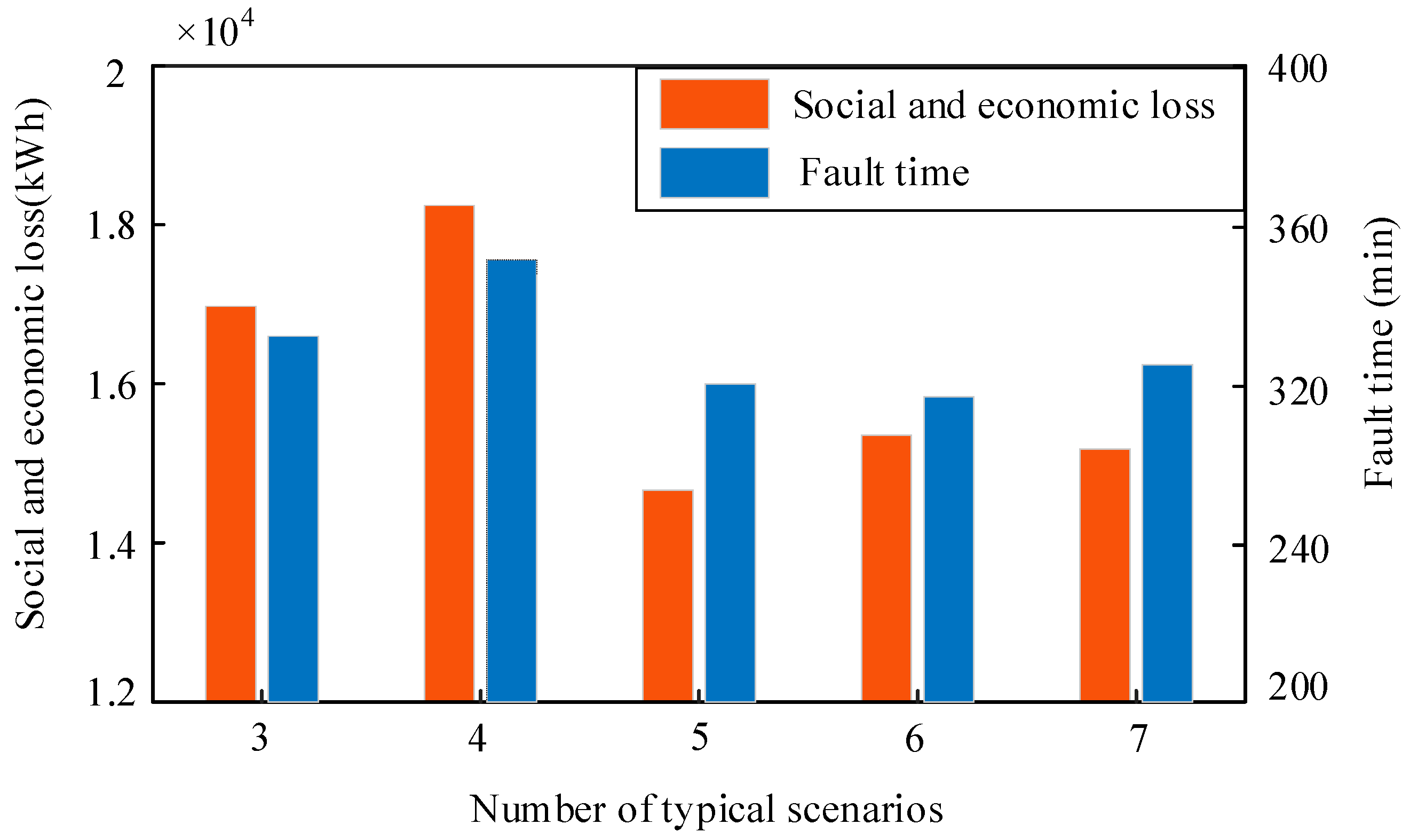
5.3.1. Analysis of Typical Scenario Numbers

The optimization results often vary with different numbers of typical scenarios. Assuming that the number of typical scenarios is 3, 4, 5, 6, and 7, Figure 10 compares the fault recovery effects for different numbers of typical scenarios. If the number of typical scenarios is too small, it is difficult to eliminate the uncertainty of DG output, which affects the recovery effect. On the other hand, too many typical scenarios increase the computational complexity, so an appropriate number of scenarios needs to be selected. From Figure 10, it can be seen that, when the number of typical scenarios increases to 5, the loss and repair time are relatively small, and further increasing the number of scenarios has little effect on the fault recovery performance. Therefore, the number of typical scenarios is set to five.

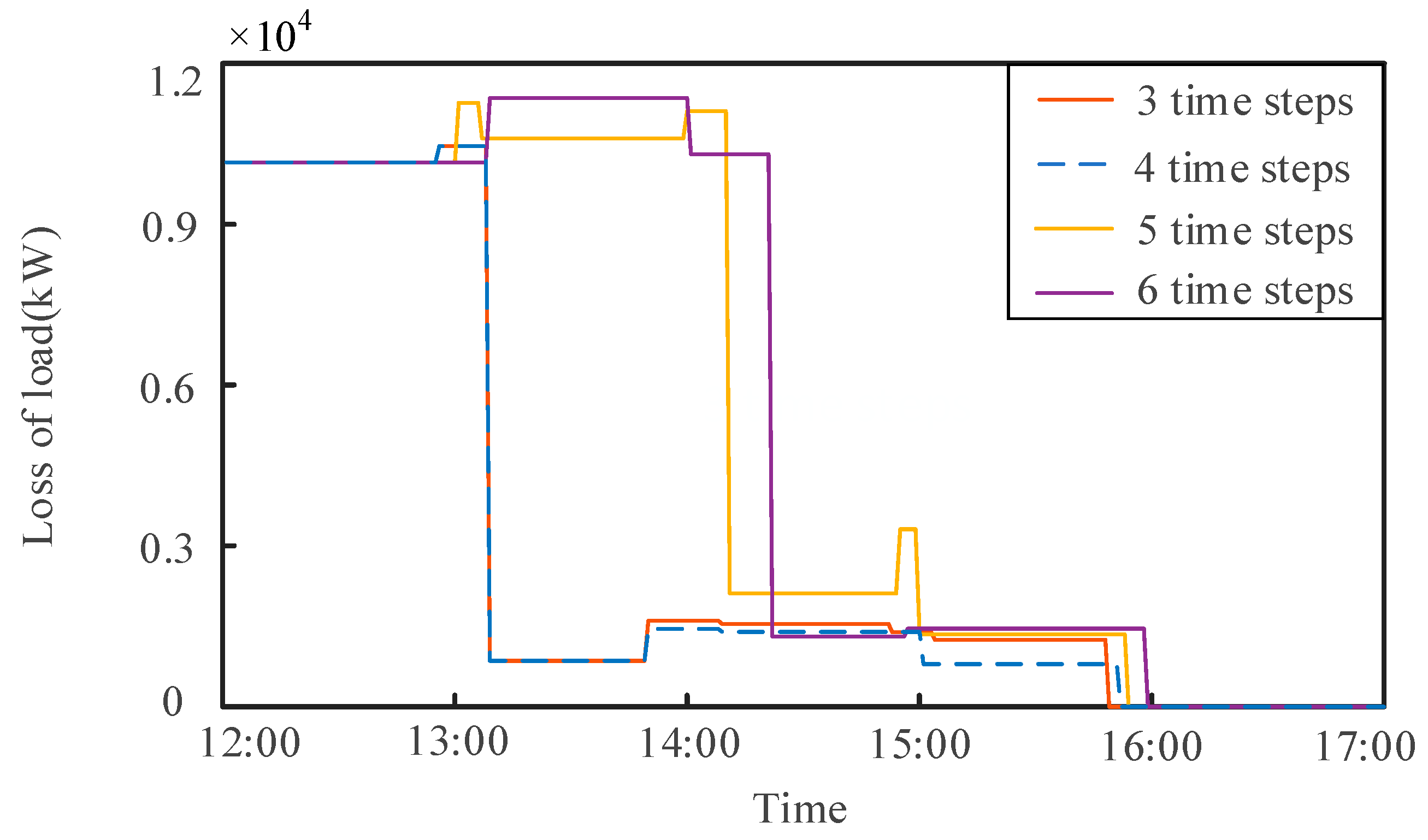
5.3.2. Prediction Horizon Analysis

To discuss the impact of different prediction horizons based on SMPC on power recovery results, we assume that the prediction horizon includes 3, 4, 5, and 6 time steps, each with a time interval of 15 min. The impact of different prediction horizons on recovery results is shown in Figure 11.

As shown in Figure 11, the impact of the multi-horizon recovery strategy based on SMPC on the recovery results was compared. It can be seen that the area below the curve corresponding to the four time steps is the smallest, which means the minimum social and economic loss, and the total time is shorter. The number of predicted time steps is not a case of the larger, the better. Suppose the number of predicted time steps is too large. In that case, the prediction error of DG output will increase, reducing the recovery strategy’s effectiveness and bringing a computational burden. Therefore, selecting the appropriate prediction horizon can better play the role of the RMPC method.

6. Conclusions

Considering the concurrent fault effect of the power side and communication side, we proposed a coordinated power–communication distribution network reconfiguration and dynamic repair joint optimization strategy. The following conclusions are described.

(1)

The power–communication coupling constraint establishes a coupling relationship between the power side and the communication side, reflecting real-time information on the power outage load, faulty equipment locations, and quantities during the fault recovery process. This provides a basis for decision making.

(2)

The proposed fault recovery strategy in this paper consists of two stages: islanding and network reconfiguration, followed by recovery. The strategy considers the impact of power–communication coupling and uncertainty. The optimization model is solved using the CPLEX solver. Simulation results based on the IEEE 33-node system demonstrate that the proposed method achieves fault recovery in power–communication coupled distribution networks.

(3)

Compared to deterministic optimization, MPC, and RMPC, SMPC reduce social and economic loss by 36.8%, 15.9%, and 5.6%, respectively, and have a relatively shorter recovery time. This indicates that, by reducing the impact of distributed generation output uncertainty, SMPC can achieve more optimal recovery plans.

The proposed method in this study addresses the challenge of cascading failures caused by power–communication coupling in distribution networks, which can impact the recovery process. Moreover, it enables accelerated load recovery and reduces power outage losses during this process. Furthermore, there is a lack of in-depth consideration of real road conditions, including traffic congestion and actual pathways, which may influence the recovery strategy. Therefore, these factors will be taken into account in future research.