Abstract
The ongoing Russia–Ukraine conflict has exacerbated the global crisis of natural gas supply, particularly in Europe. During the winter season, major importers of liquefied natural gas (LNG), such as South Korea and Japan, were directly affected by fluctuating spot LNG prices. This study aimed to use machine learning (ML) to predict the Japan Korea Marker (JKM), a spot LNG price index, to reduce price fluctuation risks for LNG importers such as the Korean Gas Corporation (KOGAS). Hence, price prediction models were developed based on long short-term memory (LSTM), artificial neural network (ANN), and support vector machine (SVM) algorithms, which were used for time series data prediction. Eighty-seven variables were collected for JKM prediction, of which eight were selected for modeling. Four scenarios (scenarios A, B, C, and D) were devised and tested to analyze the effect of each variable on the performance of the models. Among the eight variables, JKM, national balancing point (NBP), and Brent price indexes demonstrated the largest effects on the performance of the ML models. In contrast, the variable of LNG import volume in China had the least effect. The LSTM model showed a mean absolute error (MAE) of 0.195, making it the best-performing algorithm. However, the LSTM model demonstrated a decreased in performance of at least 57% during the COVID-19 period, which raises concerns regarding the reliability of the test results obtained during that time. The study compared the ML models’ prediction performances with those of the traditional statistical model, autoregressive integrated moving averages (ARIMA), to verify their effectiveness. The comparison results showed that the LSTM model’s performance deviated by an MAE of 15–22%, which can be attributed to the constraints of the small dataset size and conceptual structural differences between the ML and ARIMA models. However, if a sufficiently large dataset can be secured for training, the ML model is expected to perform better than the ARIMA. Additionally, separate tests were conducted to predict the trends of JKM fluctuations and comprehensively validate the practicality of the ML models. Based on the test results, LSTM model, identified as the optimal ML algorithm, achieved a performance of 53% during the regular period and 57% d during the abnormal period (i.e., COVID-19). Subject matter experts agreed that the performance of the ML models could be improved through additional studies, ultimately reducing the risk of price fluctuations when purchasing spot LNG.
1. Introduction
Section 1 describes the liquefied natural gas (LNG) market’s characteristics and trends. In addition, the objectives of this study are elaborated.
1.1. LNG Market Characteristics and Trends
Natural gas is a combustible gas obtained from natural sources and consists of hydrocarbons. Although natural gas (NG) components vary depending on the region and production processes, the main component is methane, which constitutes approximately 90% of NG. Generally, NG produced from gas fields undergoes a refining process to adjust its calorific value, physicochemical properties, and increase its final value as fuel. Liquefied natural gas undergoes a separate liquefaction process to cool the refined gas to below −165 °C. The volume of LNG is reduced to 1/600th of NG, which makes it easier to transport LNG carriers over long distances [1].
In 2021, global LNG trading volume amounted to 379 million tons. Australia is currently the world’s largest LNG exporter, producing approximately 80 million tons of LNG annually. Australia is followed by Qatar and the United States as the world’s second and third largest LNG exporters, respectively. The Asia–Pacific region is a major LNG consumer, importing and consuming approximately 72% of the global production. China and Japan are the world’s first and second largest LNG importers, importing approximately 81 million tons and 75 million tons annually, respectively. Korea is the third largest LNG importer, importing approximately 45 million tons annually [2]. Russia was the fourth-largest exporter of LNG in 2021, and currently holds a prominent position as a significant supplier of LNG in the global gas market [2]. However, in 2022, Russia’s LNG export capacity dropped to sixth place [3]. This decline can be attributed to disruptions in the supply of Russian gas resulting from the ongoing conflict between Russia and Ukraine. In the event of disruptions to the supply of Russian gas or sustained boycotts by gas-consuming countries of Russian gas, the international gas market will likely be adversely affected. Figure 1 shows a graph of the global LNG export and import trends, as illustrated with publicly open data from BP [2].
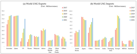
Figure 1.
World LNG exports and imports.
LNG is typically traded internationally through long-term forward contracts of 10 years or more due to the nature of LNG projects. Traditional LNG projects are large-scale projects that include the entire supply chain, including gas field exploration and development, construction of LNG liquefaction plants, and upstream to downstream processes. Integrated LNG projects require substantial investments, which differ depending on the characteristics and implementation period of a project. Typically, an investment of up to USD 1200/ton per annum is required [4]. In general, project sponsors borrow approximately 60–70% of the total investment cost from lenders through project financing (PF). The equity capital ratio of project sponsors is approximately 30–40% [5]. Under this PF structure, lenders request long-term forward contracts (LTFCs) to secure future cash flows as collateral security for their loans.
Therefore, LNG trading is globally dominated by LTFCs with contract terms exceeding 10 years. These LTFCs are typically established through commercial negotiations between sellers and buyers and have durations of at least a year. Productions outside of long-term contracts are made through short-term contracts of less than three years and spot markets, and the volumes are considerably limited compared to those of LTFCs. From the time of the construction of the first commercial LNG plant in Cleveland, Ohio, USA in 1941 [6], most LNG trading has been in the form of LTFCs, with limited activity in short-term contracts and spot LNG trading markets. However, starting in 2012, short-term and spot LNG volumes have steadily increased and currently amount to approximately 25% of the global traded volume [7]. Thus, their influence and importance is emphasized in international energy markets, where uncertainty has recently increased due to rapid climate change and ongoing conflicts.
Meanwhile, physical LNG is contractually traded with through bilateral negotiations between a seller and buyer without going through an exchange. Spot LNG is also traded in this form, and transaction information is not disclosed to the market. In particular, sales or purchase price information determines the competitiveness of LNG players and is treated as a major trade secret. Disclosing this information to parties other than those involved in the transaction is strictly prohibited.
In contrast, commodity exchanges are typically used to trade a specific commodity of equal quality in large quantities with trades made in the form of futures. Major exchanges that trade energy commodities (such as crude oil and NG) include the Chicago Mercantile Exchange (CME), New York Mercantile Exchange (NYMEX), and the Intercontinental Exchange (ICE) [8]. Most energy products worldwide are traded on open platforms, and their prices are determined based on supply and demand. Information about transactions on the platforms is generally open and easily accessible.
Recently, the Russian invasion of Ukraine and the resulting reduction in gas supplies to continental Europe have created unprecedented uncertainty in energy markets. This situation has also placed extraordinary pressure on the gas and energy markets [9]. Europe relies on Russian gas imports for more than 45% of its NG demand. Consequently, the prolonged conflict in Ukraine has fueled uncertainty regarding NG supply and demand in the UK, leading to a significant increase in NG prices in the European market. As of 6 October 2022, the National Balancing Point (NBP), Europe’s leading NG price index, was 36.40 USD/Metric Million British Thermal Unit (MMBtu) and the Title Transfer Facility (TTF) was 52.34 USD/MMBtu [10].
Due to its political and geographical characteristics, Korea relies on LNG imports for nearly all domestic NG consumption. Therefore, the country is facing a supply burden owing to the rise in NG prices caused by recent international changes, as well as increased demand in winter. In particular, NG power plants are responsible for meeting peak demands in Korea’s power supply system. Accordingly, to respond to growing electricity demand during specific periods (e.g., winter), it is essential to purchase spot LNG. Korea procures over 90% of its LNG imports through long-term contracts and less than 10% of its remaining volume through spot LNG purchases. However, the recent unusual temperature changes have an effect on spot LNG purchases, resulting in instances where such purchases exceed 10% of the total supply.
In summary, the global LNG market is complex and constantly evolving, shaped by various factors such as geopolitical tensions, climate change, and supply and demand dynamics. The increasing importance of short-term and spot LNG trading has highlighted the need for efficient risk management strategies in the LNG industry.
1.2. Problem Statement and Research Objectives
In Europe and North America, where pipeline systems are well-developed, the main market is based on NG rather than LNG. Therefore, the European and North American markets have developed and established their own price indexes (including NBP and Henry Hub (HH)) that serve as references for NG transactions. In contrast, in the Asia-Pacific region, the development of intercontinental pipeline systems for supplying NG is insufficient due to regional political and security considerations [11]. With the exception of China, the major Asia–Pacific LNG consumers including Korea, Japan, and Taiwan have been unable to secure gas supply sources by constructing pipeline systems throughout the region, as has been done in Europe and North America. Therefore, they rely on LNG imports for most of their gas supply [12]. Consequently, the region has not developed its own NG price indexes. With market characteristics such as the LTFC method in LNG trading, the Asia-Pacific region has used variable prices in the form of price formulas, with crude oil price indexes serving as linked variables. Examples of these include Japanese customs cleared (JCC) crude oil and Indonesian crude price (ICP), rather than NG indexes.
Unlike LNG trading through LTFCs, spot LNG is traded in units of LNG carriers. A fixed price (unit: $/MMBtu) is set based on the price per calorific value of LNG. Although the spot LNG market has grown to approximately 25% of the global trading volume over the last decade, the product supply flowing into the spot market is undeniably insufficient. Starting from February 2009, Standard and Poor’s global commodity insights named the spot LNG traded in Asia as the “Japan Korea Marker (JKM)” and began evaluating daily spot LNG prices [13]. The fact that a spot LNG price index was first announced in 2009 indicates the spot LNG market’s inactivity. Spot LNG exhibits relatively large price fluctuations depending on changes in demand and supply, owing to fundamental limitations caused by supply liquidity constraints. Figure 2 shows a graph of the fluctuations in JKM, HH, and NBP, which are major NG price indexes, over the past 10 years [14,15,16]. Until the early 2000s, these three indexes exhibited a decoupling trend with repeated fluctuations, with JKM experiencing the most prominent range of fluctuations. From 2014, JKM experienced a significant decline and then merged with NBP and HH again; however, its volatility remained relatively high. In contrast, HH exhibited slight fluctuations and the most stable trend. Therefore, based on the trends of the past 10 years, JKM is highly volatile compared to other NG indexes, and this volatility persists to date.
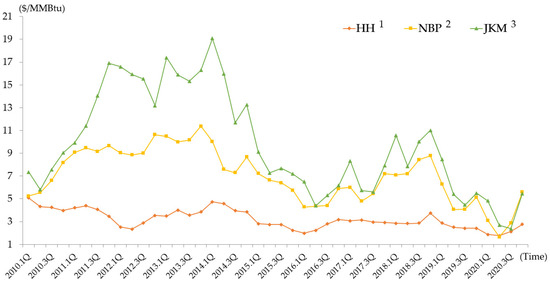
Figure 2.
Historical trends of JKM, HH, NBP for ten years. 1 HH: henry hub. 2 NBP: national balancing point. 3 JKM: Japan Korea marker.
Under these market conditions, LNG buyers address their peak demands through spot LNG purchases. Buyers forecast annual, quarterly, and monthly demand, taking into account their country’s temperature and planned maintenance schedules for base–load power generation. To secure the required quantities, which are calculated through sophisticated demand forecasting, buyers establish and implement procurement plans reflecting market conditions. Practitioners typically make spot LNG purchases using qualitative criteria based on domain knowledge and market conditions. However, the lack of objective quantitative criteria can delay decision making, thereby exposing them to price fluctuation risks. Developing quantitative criteria to support decision-making for spot LNG purchases is expected to reduce exposure to purchase price fluctuation risks and ultimately lower NG purchase costs.
This study aimed to develop a spot LNG price prediction model based on machine learning (ML) algorithms to reduce purchase price fluctuation risks for spot LNG imports into South Korea. The following are the categories of key features used to predict the JKM spot LNG price index:
- international NG prices
- international crude oil prices
- LNG import volumes by country
- average temperatures of key Asian countries
- LNG export volumes by country
Long short-term memory (LSTM), artificial neural network (ANN), and support vector machine (SVM) algorithms, which are mainly used in time series prediction modeling, were used to develop ML-based prediction models. This study is the first to develop a JKM prediction model and compare its performance with that of the autoregressive integrated moving average (ARIMA), a traditional statistical prediction technique. Furthermore, to test the developed model’s price prediction performance, the authors divided the dataset into before and after the COVID-19 outbreak to measure its performance for both periods to reflect realistic circumstances in the research results. Finally, this study introduced a new method for interpreting prediction results and presented a practical application for the developed ML model. Forecasting spot LNG price trends based on the results of this study is expected to reduce the price fluctuation risks associated with spot LNG imports into Korea and ultimately reduce NG prices.
This paper consists of 10 sections. Section 1 describes the LNG market’s characteristics and trends, as well as the study’s necessity and purpose. Section 2 analyzes research conducted on crude oil and NG price prediction using ML techniques, as well as studies applying ML prediction techniques to stocks, virtual currencies, and exchange rates. Additionally, it examines prior research using traditional prediction techniques for time series data. Section 3 describes this study’s scope and framework. Section 4 presents an overview of the methods and modeling and explains the collection of data used in JKM prediction, feature selection, preprocessing, and modeling. Section 5, Section 6, Section 7 and Section 8, which are the most important parts of this paper, analyze the training and testing process and present the results of predicting JKM through a scenario analysis using the developed ML models. Section 9 summarizes the results of this study and their major implications. Finally, Section 10 analyzes the limitations of this study and concludes the article with suggestions for future research to improve the performance of the models.
2. Literature Review
Section 2 analyzes research on crude oil and NG price prediction using ML techniques, as well as studies applying ML prediction techniques to stocks, virtual currencies, and real estate prices. In addition, it explains previous research using traditional prediction techniques for time series data. Through the literature review, the authors identified the ML algorithms commonly used to predict time-series data and defined the limitations of previous research and the necessity of this research.
2.1. Energy Prices Prediction Using ML Algorithms
The authors reviewed previous literature on predicting energy prices, such as crude oil and NG, using ML techniques. To predict crude oil prices, Gao and Lei presented a stream learning method and a new ML paradigm and developed a model that can be continuously updated using new oil price data [17]. Su et al. applied ANN, SVM, gradient boosting machines (GBM), and Gaussian process regression (GPR) techniques to HH spot price prediction, an NG price index in North America. According to their results, the ANN method yielded a better predictive performance than other ML algorithms [18]. Xian et al. studied crude oil price prediction using an SVM, ANN, and hybrid EMD–SVM. The results showed that the proposed hybrid EMD–SVM model yielded excellent performance compared to prediction models using individual algorithms, and that the predictive performance for oil prices was substantially improved using the hybrid model [19]. Gupta and Nigam studied crude oil price prediction using an ANN algorithm and identified the optimal lag and number of delay effects of the ANN algorithm. Consequently, unstable patterns of crude oil prices were continuously captured, which significantly enhanced the model’s predictive performance [20]. To explore the optimal prediction model for Korean LNG import prices, Seo applied various econometric models, including autoregressive integrated moving average with exogenous variables (ARIMAX), vector error correction model (VECM), the ML algorithm LSTM, and a hybrid model that combined the two models. According to the tests on each model, VECM–LSTM was selected as the optimal model, with high prediction accuracy and interpretability [21]. Mouchtaris et al. used SVM, regression trees, linear regression, GPR, and an ensemble of tree ML models to predict the spot prices of NG after 1, 3, 5, and 10 days. According to the results, the SVM model yielded the best predictive performance [22]. Fetih and Balkaya investigated the history of crude oil price predictions and the application of artificial intelligence (AI) techniques. They concluded that ANN algorithms were the most suitable for complex and sensitive oil price prediction, considering their hierarchical structure that can relate the target variables and numerous parameters in detail. Furthermore, they found that the prediction results could be improved by applying text mining in combination with other methods [23]. Kaymak and Kaymak conducted research on enhancing the predictive performance of oil prices during COVID-19 by improving models using ANN and SVM algorithms. They proposed a novel method that combined fuzzy time series and the greatest integer function with existing ANN and SVM models. The researchers found that the proposed model outperformed existing models that used the two algorithms alone [24]. Tschora et al. (2022) investigated the latest ML techniques to accurately predict day-ahead electricity prices in Europe, where electricity price volatility is high due to various energy production sources and storage difficulties. They added previously unused new features, such as price histories of multiple neighboring countries, to the datasets, which dramatically increased the model’s performance. DNN and SVR were found to extract meaningful information from the features and cope with market changes such as gas price prediction [25]. Tan et al. proposed a new hybrid deep learning-based model called convolutional neural network (CNN) + stacked sparse denoising auto-encoders (AE) to address the technical difficulties in accurate price prediction due to the nonlinearity, randomness, and volatility of electricity prices. The study experimented with the Australian national electricity market as a case study and showed outstanding prediction performance for price spikes. Additionally, the proposed model can save training time for neural networks in the prediction process [26]. Qin et al. compared popular single-model and multiple-model ML methods used for crude oil price prediction by applying online data from Google Trends to enhance the prediction ability. The experimental results indicated that introducing Google Trends can improve prediction performance, and the multiple-model approach indicated higher prediction accuracy [27].
2.2. ML Applications for Price Prediction Based on Time Series Data
The authors reviewed the previous literature on price predictions of other goods using ML techniques. Researchers have conducted price prediction studies on various commodities and goods such as stocks, options, cryptocurrencies (e.g., Bitcoin), and real estate prices. Ramakrishnan et al. used SVM, neural networks, and random forest (RF) ML techniques to analyze the impact of the prices of four commodities (crude oil, palm oil, rubber, and gold) on the Malaysian exchange rate. They found that the RF technique was superior in terms of accuracy and performance, and that the price of the four commodities was a strong dynamic parameter influencing the Malaysian exchange rate [28]. Fu et al. studied exchange rate predictions for four currencies (USD, EUR, JPY, and GBP) using an evolutionary SVM (E-SVM). Furthermore, they developed two regression models based on the E-SVM algorithm and evaluated their exchange rate predictive performance. The results showed that E-SVM outperformed all other benchmark models in terms of the prediction level accuracy, prediction direction accuracy, and statistical accuracy [29]. Vijh et al. applied ML techniques to predict the stock closing prices and next-day stock prices of five companies (Nike, JP Morgan, Goldman Sachs, Johnson & Johnson, and Pfizer) using ANN and RF ML models. They used six variables comprising historical time-series data to train ML models. The analysis results showed that the ANN model outperformed the RF model [30]. Truong et al. compared the performances of traditional and advanced ML models in predicting housing prices in Beijing by applying RF, extreme gradient boosting, a light gradient boosting machine, hybrid regression, stacked generalization algorithms, and 19 variables. Based on the analysis results, they suggested the need for additional research on hybrid models to supplement the different strengths and weaknesses of each model [31]. Kim et al. conducted a study to predict Ethereum prices, a major cryptocurrency, using ML techniques based on blockchain information. According to an analysis using ANN and SVM models, ANN outperformed SVM. Moreover, the most suitable independent variables for predicting Ethereum prices were macroeconomic factors, Ethereum-specific blockchain information, and Bitcoin cryptocurrency blockchain information [32]. Choi et al. developed an engineering machine learning automation platform (EMAP) that applies AI and big data technology to predict risk at different stages in the life cycle of oil and gas engineering projects. Among EMAPs, M2 is a design cost estimation module modeled using Decision Tree, Random Forest, Gradient Boosting, and XGBoost algorithms. As a result of the evaluation, Random Forest was found to be the best model [33]. Kurani et al. evaluated the applicability of these algorithms to stock predictions by conducting a study on stock price prediction using ANN and SVM models. The results showed that both algorithms solved common constraints in stock prediction, such as time windows, data constraints, and cold starts. Furthermore, the hybrid model further improved the predictive performance [34]. Chhajer et al. conducted case studies by applying AI and ML to stock market predictions. They classified cases of stock market predictions using ANN, SVM, and LSTM algorithms. Based on the analysis results, it was concluded that ML models can efficiently process historical data, trend lines, and charts, making them suitable for predicting future market trends. They also demonstrated that the ANN, SVM, and LSTM algorithms were the best in the field [35]. Xiong and Qing proposed a new hybrid forecasting framework that combines VMD with time series prediction to improve the forecasting accuracy of day-ahead electricity prices. The new framework introduced an adaptive copula-based mutual information feature extraction (ACBFS) method based on conditional mutual information (MI). It is also a day-ahead electricity price forecasting (EPF) model that combines variational mode decomposition (VMD) with a Bayesian optimization and hyperband (BOHB)-improved LSTM neural network [36]. Iftikhar et al. compared several decomposition techniques for various time series models to forecast time series properties that are difficult to model. They proposed a new prediction methodology after comprehensively analyzing monthly electricity consumption predictions. This study employed data on Pakistan’s monthly electricity consumption from 1990 to 2020 and found that the proposed method outperformed the benchmark seasonal trend decomposition (DSTL) [37].
2.3. Comparison of Traditional and ML Methods
The authors reviewed previous literature comparing the performance of traditional and ML methods for predicting time series data. Gosasang et al. conducted research on predicting the volume of container throughput in the Bangkok port using a multilayer perceptron (MLP) and linear regression. They found that MLP is superior in terms of accuracy and performance [38]. Siami-Namini and Namin compared the performances of ARIMA and LSTM models for time-series data. For financial time series data, the LSTM model had a root mean square error (RMSE) score of 87% lower than that of ARIMA, and for economic data, it scored 84% lower and revealed that the ARIMA model underperformed the LSTM [39]. Makridakis et al. studied concerns regarding statistical and ML prediction methods and suggested directions for moving forward. They found that conventional statistical methods were more accurate than ML. The ML performance has a significant effect on the length (size) of the dataset used, and the longer the length, the better the training of the ML model is optimized [40]. Sagheer applied deep LSTM (DLSTM), a deep gated recurrent unit (DGRU), and ARIMA models to predict the production data of real oilfields. A comparison of the performance of each model revealed that DLSTM outperformed the statistical model ARIMA on nonlinear prediction problems [41]. Guo conducted oil price research using deep learning and ARIMA models. The convolution neural network model is fast in training and has the performance accuracy of the LSTM and gated recurrent unit (GRU). They proposed combining neural network models and traditional seasonality models to improve performance [42]. Calkoe et al. applied ML and traditional methods for sand beach predictions. Despite exhibiting comparable performance to traditional methods described in the research, the performance of ML algorithms is heavily reliant on the quality of data.. ML has an efficient advantage in terms of computing time [43]. Poggi et al. compared traditional inferential statistical methods and newer deep learning techniques for forecasting electricity prices in the German market during highly volatile periods, such as 2020 to mid-2022. While this study did not report that any particular model was superior, it suggested that combining statistical and neural network (NN) models can be used an alternative approach [44].
2.4. Limitation of Previous Research
Owing to advancements in information technology, AI has been used in various industries. Among AI technologies, ML techniques are actively incorporated and utilized in diverse fields and items, from predicting energy prices (crude oil, NG), financial goods prices (stocks, options, cryptocurrencies), and weather (rainfall and snowfall) to battery life. However, energy price studies that apply ML techniques are lacking. In particular, there is a lack of research on the application of ML technology to the NG industry sector, and no research exists on spot LNG price prediction. Moreover, the studies do not properly reflect the unique circumstances in which uncertainty considerably increased due to the COVID-19 pandemic. In addition, in the case of the ML model, it was found that the dataset length used for the ML model had the largest effects on the ML performance, and that the ML model could perform better than the traditional method when it could not use a dataset of sufficient length.
Accordingly, this study developed a prediction model for JKM: a spot LNG price index using LSTM, ANN, and SVM algorithms, which are primarily used in prediction research based on time-series data. The authors validated the developed ML models by comparing them with ARIMA, a traditional statistical model, and measured their predictive performance during the COVID-19 period to reflect realistic circumstances in the research results. Additionally, the authors compared the ML technique with existing practices to secure legitimacy and examine its practical applicability.
3. Research Scope and Framework
Section 3 describes the scope and framework of this study. It presents the core objective and methods used in the study.
3.1. Scope of Work
This study aims to develop a spot LNG price prediction model based on ML algorithms to reduce the purchase price fluctuation risk for spot LNG imports into Korea. The scope of this study is as follows:
First, the authors developed a JKM prediction model using ML algorithms such as LSTM, ANN, and SVM, which are commonly used for time-series data prediction. The authors then used the developed ML models to predict JKM after N + 1, 5, and 10 d and measured the mean absolute error (MAE), mean absolute percentage error (MAPE), and RMSE scores, which are regression model performance indicators, to determine their prediction accuracy. The authors also validated the developed ML models by comparing their performances with that of ARIMA, a traditional statistical model. Second, in this study, the independent variables used in the training of the ML prediction model were limited to the following eight factors:
- JKM, spot LNG price index
- NBP and NG price index in Europe
- HH and NG price index in North America
- Brent: Major crude oil price index.
- LNG import Volumes of Korea
- China’s LNG import volumes
- LNG import Volumes of Japan
- Average temperatures in Seoul, Korea
Third, the data collected and processed for this study were unstructured numerical data derived from daily published price information. Taking into account the nature of statistical numerical data, the authors collected monthly data on LNG imports for each country. The import volume information for each country was pre-processed and converted into a daily sequential term.
Fourth, unstructured text information, such as headlines from daily newspapers related to the LNG business, was excluded from the data collection for JKM prediction. Finally, the authors developed a JKM prediction model to support quick and accurate decision-making in spot LNG purchases.
3.2. Research Framework
This study was conducted following the procedure described below. Section 4 explains the collection of the background dataset that served as the basic data for the spot LNG price prediction model, preprocessing, feature selection, and splitting of the dataset to train and test the ML models. Spot LNG-related energy price index information (JKM, Brent, HH, and NBP) was extracted using the KOGAS data package system (KDPS). Data on the daily average temperatures of the capital cities of Korea, China, and Japan, which are major LNG importers in the Asia–Pacific region, were collected from the Open MET Data Portal (OMDP) of the Korea Meteorological Administration (KMA). The authors organized the collected data in Microsoft Excel to facilitate uploading and loading process while developing the ML model code. This step also involved explaining the feature selection process, which included a workshop with subject matter experts (SMEs) and the preprocessing step to construct datasets for training and testing the ML models using the raw data. The preprocessed dataset was divided into normal and subsequent abnormal periods, serving as the training and test sets for the ML models.
Section 5, Section 6, Section 7 and Section 8 provide an explanation of the training, testing, and validation processes for the ML models used in spot LNG price prediction. To train the ML models, the authors established and analyzed four scenarios with dimensions of 1, 2, 7, and 8. Initially, the authors varied the combinations of independent variables to match the conditions of the ARIMA model as closely as possible, based on each test result. Subsequently, three additional scenarios were analyzed. Three algorithms (LSTM, SVM, and ANN) were employed to develop the prediction models using ML techniques. The performance indicators of regression models (MAE, MAPE, and RMSE) were used to assess the accuracy of price predictions made by the ML models. Finally, the models were validated by comparing their performance with that of the traditional statistical prediction model, ARIMA. As a result, the authors derived an optimal prediction model based on ML algorithm.
Section 9 presents the conclusions and limitations of this study and future research directions. Figure 3 illustrates the process of developing the spot price prediction models described above.
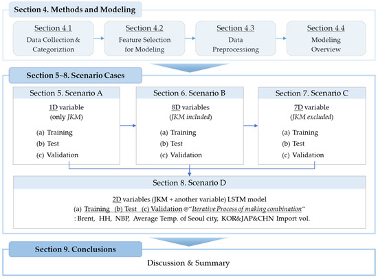
Figure 3.
The model development process.
4. Methods and Modeling
Section 4 presents an overview of the methods and modeling and explains the collection of data used in JKM prediction, feature selection, preprocessing, and modeling.
4.1. Data Collection and Categorization
The background dataset used for this study was extracted through KDPS, and the temperature data were collected through the OMDP of KMA [45]. The collection period for extracting the raw data was set to 12 years, from 2010 to 2021.
During the data collection, we initially considered including financial market indexes, such as exchange and interest rates, as a major category of the basic data. However, upon incorporating these variables into the predictive models developed in this study, we found that they did not significantly improve the models’ predictive power. Consequently, we opted to focus on collecting basic data primarily from the following five categories commonly used in short-term natural gas market forecasting within the industry, excluding the aforementioned financial market indexes.
First, the raw data collected for the 87 variables were classified into five categories. Table 1 lists the categories. The classification criteria and details are as follows:

Table 1.
The categories of the raw dataset.
Category A, a group of international NG price indexes, was extracted through the KDPS. The collection period for extracting the raw data was set to 12 years, from 2010 to 2021. The most important information in this study included data on JKM and the spot LNG price index set as the prediction targets. JKM is announced in LNG Daily, a newspaper published by Platts under S & P Global. A spot LNG price index for the Asia–Pacific region, JKM, was announced in 2009 based on spot LNG transaction information in Korea, China, Japan, and Taiwan, which are major LNG importers [13]. For spot LNG trading in the same region, sellers and buyers generally check the day’s JKM price, predict demand according to power generation, climate change, and energy market conditions related to each country, and negotiate the purchase price considering the demand and supply of spot LNG in the market. Because JKM information is the most crucial data used in this study, its importance can be regarded as very high. The gas market price indexes of each region influence spot LNG prices. Major international NG price indexes include NBP and TTF, which represent the European NG market, and HH, the benchmark price of the North American NG market. Depending on the prices in Europe and North America, the volume of spot LNG traded in the Asia–Pacific region may divert to either market. Considering that the supply and demand conditions of each market organically influence each other, this is classified as basic information for predicting JKM.
Category B, a group of international crude oil prices, was extracted from the KDPS. The collection period for extracting the raw data was set to 12 years, from 2010 to 2021. As of 2021, approximately 63% of LNG transactions worldwide have been in the form of LTFCs [46]. Owing to the nature of this contract type, signing an LTFC at a fixed price exposes both the buyer and seller to excessive risk. Therefore, rather than fixed prices, the LNG industry trades based on a floating price structure in the form of a formula linked to crude oil price. Because fluctuations in international crude oil prices significantly influence LNG prices, international crude oil price information was collected in the form of important background data.
Category C, a group of LNG import volumes by country, was extracted using the KDPS. The collection period for extracting the raw data was set to 12 years, from 2010 to 2021. The import volume data of LNG importers worldwide are objective information through which each country’s LNG demand and consumption patterns can be estimated. LNG is typically traded in the over-the-counter (OTC) market, that is, trades are made directly between the seller and buyer without going through an exchange [47]. Spot LNG is traded in this manner. LNG buyers and sellers are concerned about a decrease in their bargaining power for purchasing prices owing to position exposure; hence, the leakage of buyers’ demand information and sellers’ supply information is strictly controlled, making it difficult to access this information. As an alternative, this study collected data on country-specific LNG import volumes, which provide objective statistical information, and analyzed their impact on JKM. In particular, the authors determined that there would be a meaningful link between the LNG import volume information of major countries in the Asia–Pacific region and the prices of spot LNG traded in the region.
Category D, a group of the average temperatures of major LNG importing countries in the Asia–Pacific region, was extracted through the KMA’s OMDP [48]. The collection period for extracting the raw data was set to 12 years, from 2010 to 2021. The country-specific LNG import volume, classified into the primary data group above, was determined by changes in supply and demand conditions due to temperature changes in each country. Therefore, the average temperature data of major countries in the Asia–Pacific region, the core of the LNG market, were classified as significant in this study. The average temperature information was collected for each country’s capital city, which is densely populated, assuming that it represents changes in demand in each country. This information was collected through the KMA’s OMDP separately from previous data.
Category E, a group of LNG export volumes by country, was extracted using the KDPS. The collection period for extracting the raw data was set to 12 years, from 2010 to 2021. These data can be used as basic information to represent global LNG supply. Similar to the above-mentioned LNG import volume information, it is impossible for LNG players other than actual LNG producers to immediately check or collect information on the detailed production profiles of specific liquefaction plants or planned and unplanned maintenance schedules in liquefaction plants. These events ultimately impact production volume and can significantly influence commodity prices in markets with liquidity constraints, such as spot LNG markets. Indeed, the spot LNG price traded during a specific period often increases when an unplanned shutdown of a specific LNG plant occurs. Moreover, by excluding these uncontrollable circumstances, the spot LNG price fluctuates significantly when the purchase volume of a specific country, buyer, or seller grows rapidly, or the supply volume decreases. Accordingly, the authors determined that changes in LNG supply could be reasonably estimated using each country’s LNG production information based on statistical data. Therefore, they collected and classified this information.
4.2. Feature Selection for Modeling
Feature selection refers to the process of obtaining a subset from an original feature set according to a certain feature selection criterion that selects the relevant features of the dataset [49]. It plays a role in compressing the data-processing scale, where redundant and irrelevant features are removed. Good feature selection results can improve learning accuracy, reduce learning time, and simplify learning results [50]. It is challenging to quantify the influence of the collected data on spot LNG prices. Consequently, the authors conducted a workshop to gather insights from SMEs in the NG industry and selected the features based on their inputs. The expertise of the SMEs, derived from industry practices and their extensive work experience in related fields, greatly influenced the selection of features that impact spot LNG prices. The workshop included two SMEs with over 20 years of experience in the NG industry and five SMEs with over 10 years of experience. Based on the workshop results, the authors initially identified features estimated to have the most significant impact on JKM. From this initial group, features that had a suitable form for predicting JKM using ML models were selected. As a result, eight independent variables were chosen from these five categories.
First, three variables, JKM, HH, and NBP, were selected from category A: international NG prices. JKM is the spot LNG price index of the Asia–Pacific region, and was the prediction target in this study. HH and NBP are the representative NG price indexes for the North American and European markets, respectively. According to the Asian spot LNG market price, the LNG volume produced or re-loaded in the area is diverted to Asia, and spot prices influence each other. Therefore, they were selected as significant variables.
Second, the Brent variable was selected from category B, which represents international crude oil prices, for several reasons. Owing to the development of pipeline infrastructure systems in each region, NG is more actively traded than LNG and has formed a mature and transparent market. Therefore, trading is conducted using its own price index developed for each trading region. Conversely, LNG does not have its own price index and is traded based on a formula linked to crude oil prices. Considering that the first commercial LNG was produced in 1940, price structures linked to the JCC or ICP have been most commonly used in the Asia–Pacific region. From the early- and mid-2000s, the Brent price, which is relatively advantageous for hedging, was used for LNG trading. Compared to the JCC or ICP, Brent has an abundant volume and a mature trading market, which facilitates hedging. Consequently, many LNG players have recently preferred to use the Brent price index. Reflecting this trend, the authors selected it as an important factor that influences spot LNG prices.
Third, the LNG import volumes of three Asian countries were selected as variables from category C. China, Japan, and Korea are the world’s first, second, and third largest importers respectively. This selection was made based on the understanding that the volumes of these major LNG importers worldwide have a significant influence on spot LNG prices.
Fourth, the average temperature of Seoul, the capital of Korea, was selected as a variable from category D. Furthermore, the authors collected the average temperature data of the capital cities of China and Japan, the largest and second-largest LNG importers, through the KMA WDSP. However, due to inconsistent data intervals and many missing values, it was necessary to impute the data. This process significantly distorted the data. Therefore, the authors excluded these variables from the final selection.
Fifth, the export volume data of LNG producers were excluded from the final variable selection for category E. Initially the authors collected this data with the intention of objectively evaluating LNG supply based on the changes in export volume of LNG producers. However, the SMEs pointed out it was nearly impossible to track how much of each producer’s export volume specifically flowed into the Asia–Pacific region. As a result, the authors took their opinions into account and decided to exclude the data. Another reason for excluding the data was the issue of data distortion caused by correcting missing values. The LNG export and import volume data are based on statistical data, with the smallest units being on a monthly basis. In contrast, JKM (the prediction target) is collected on a daily basis, requiring the transformation of missing value into a daily sequence term. Although missing values can be corrected through rational estimation (such as linear interpolation), the authors believed that this process would unavoidably introduce data distortion due to increase in processed data values. Additionally, the authors hypothesized that increasing the number of variables with these characteristics would significantly impact the final results analyzed in this study. Therefore, no additional variables were included in this category. Table 2 provides a list of the eight variables selected through the aforementioned feature selection process.
Table 2.
The list of selected variables.
4.3. Data Preprocessing
Important information must be extracted from the data to develop a prediction model for specific data. For this purpose, data preprocessing is performed, wherein the researchers process the analysis data using their own knowledge [51]. This process varies depending on the characteristics of the data, and there is no single standardized procedure or correct answer. Therefore, a suitable pre-processing method must be selected based on this study’s requirements. In this study, the data collected and selected to predict spot LNG prices consisted of time-series data, and the programming language used for preprocessing was Python. Pandas and NumPy libraries provided by Python were used to create a data frame in the form of a two-dimensional array, which was collected to train and test the ML models. The dataset of variables finally selected and used for modeling was in the form of a Microsoft Excel sheet. The file was loaded using Python 3.7, after which a two-dimensional data frame of the dependent and independent variables was created. First, missing data were identified by inspecting the information in the data frame, and then the values were imputed. Second, the data format was converted to create an input for the model. To match the data input format of the time-series prediction model, the existing data were reconstructed into a three-dimensional format of “window sample number, time step, features”. The data were also converted into lookback (past steps) and look forward (future steps) formats for the input of the LSTM model. Finally, the data were standardized to complete preprocessing. As the variables used for spot LNG price prediction had low multicollinearity, the authors did not conduct a correlation analysis between the variables. The datasets collected and used in this study comprised daily and monthly numerical information based on public announcements and statistical data; hence, it was not necessary to eliminate noise. Moreover, denoising was not included in the preprocessing because it could damage the original data and cause distortion.
4.3.1. Missing Value Imputation
As the name implies, a missing value is one that does not exist [52]. Missing values in data reduce analysis efficiency, introduce complexity in data processing and analysis, and cause bias due to the difference between missing values and complete data. Therefore, missing values make data analysis more difficult [53]. In most cases, simple techniques are applied to handle missing data, which sometimes produce biased results. In contrast, imputation techniques can be applied to produce valid results without complicating the analysis [54]. For the energy price indexes used in this study, considering that announcements are not made on non-business days (such as national holidays), there is no price information for these days. Such missing values are generally eliminated if they do not significantly influence the dataset composition. However, removing missing values from time series data can cause statistical distortions in the mean, variance, and other parameters at the corresponding time points, thereby affecting the data analysis results.
Accordingly, to conduct smooth time-series data analysis, it is important to replace these missing values and convert the sequence term. The energy price indexes used in this study (JKM, Brent, NBP, and HH) have missing values by nature, considering that they are announced only on business days. Moreover, although the LNG import volume data for major Asian countries do not contain missing values, they are in the form of monthly data based on statistics. Therefore, they must be converted to daily data, the same unit as JKM, which is the prediction target of the ML prediction models.
Techniques to replace missing values in time-series data include forward-fill, which replaces a missing value with the previously observed value; backfill, which replaces a value with the next observed value; and the moving average/median method, which replaces a value with the average value/median of the previous n time windows. If a missing value is in a section where the preceding and following pattern changes is replaced with the above methods, the replaced value may differ from the actual value, thereby causing problems in the analysis. In such cases, the missing values can be handled using linear interpolation. Linear interpolation involves utilizing data already obtained statistically to infer the value between time t and t + 1. Considering the characteristics of each dataset with missing values, the authors applied linear interpolation to all missing values. For price indexes, it is common to use the value announced on the previous business day for the missing value on an unannounced day. Replacing missing values with the backfill method may cause distortion when using unannounced values in the future. Although using linear interpolation can cause errors by applying assumed values based on increasing or decreasing trends, this effect was ignored, considering that there were very few missing values in the obtained dataset. Therefore, linear interpolation was applied to all missing values in this study to improve preprocessing efficiency. However, the values for 1 January 2010, the starting point of the data used in this study, were replaced using the backfill method. Next, it was necessary to convert the LNG import volume data from monthly to daily. The import volume in a certain month may increase, decrease, or (in very few cases) remain unchanged in the next month. Based on the assumption that these numerical changes were linear, the authors converted the monthly figures into daily data through linear interpolation.
The present study sought to simplify country-specific patterns of LNG imports based on monthly data and eliminate potential noise that could arise during the conversion to daily data. Linear interpolation was identified as a suitable method to minimize distortion of the existing data while also offering the advantage of being easily verifiable by others. As such, linear interpolation was applied uniformly to preprocess tasks such as converting monthly data into daily data and correcting data gaps. This ensured that the resulting data were both accurate and reliable for subsequent analysis. There were no missing values in the daily temperature data for Seoul, the capital city of Korea.
4.3.2. Reshape and Standardization of Input Data
The data were converted to lookback (past steps) and look forward (future steps) formats for the input of neural network algorithm-based models, such as LSTM and ANN. In other words, to match the data input format of the LSTM model, the data were reconstructed into a three-dimensional format of “data size, time step, features”. “Time steps” indicates the number of columns in one data and “features” indicates the number of lows to input at once [55]. Reshaping the input data in this manner is essential for training the LSTM model.
Most ML algorithms yield a better performance when the input variable data are scaled. The most common scaling methods for numerical data prior to modeling are normalization and standardization. Normalization involves individually adjusting the size of each input variable to the most accurate floating-point value range, that is, zero to one [56]. Standardization adjusts the scale of each input variable by subtracting the mean and dividing the result by the standard deviation [56]. Therefore, it shifts the distribution such that the mean and standard deviation are zero and one, respectively. Data scaling is a recommended preprocessing step for ML algorithm models to improve the performance of predictive model algorithms. The scaling method for the input variable data varies with the details of the problem and the characteristics of each variable [56]. This study standardized the data using StandardScaler from the scikit-learn library.
4.3.3. Split of Training and Test Dataset
Based on the ML models using various algorithms, it is necessary to appropriately classify the dataset according to the purpose of selecting the optimal model and verifying its performance. In a data-rich situation, the best approach is to randomly classify the preprocessed data into training, validation, and test sets. The training set was used to fit the model, the validation set was used to measure performance (estimate prediction error) for selecting the optimal model, and the test set was used to measure the generalization error of the selected optimal model [57].
The background dataset used for this study was extracted using KDPS. The collection period for extracting the raw data was set to 12 years, from 2010 to 2021. As the first step in classifying the dataset, considering the impact of COVID-19, data from 2010–2019 and 2020–2021 were divided into normal and abnormal periods, respectively. The normal period data were then classified into training and test sets at an 8:2 ratio to train and test the ML prediction models. Abnormal period data can be judged as outliers and excluded from the dataset classification. However, the authors separately prepared data for COVID-19 to further validate each model’s predictive power under rapidly changing market conditions. A separate validation set was not considered due to the limited size of the collected dataset.
The JKM index, which is the prediction target of ML models, was first introduced to the market in 2009. At this time, owing to the low reliability of the index, it had problems including abnormal fluctuations and insufficient data. Therefore, 2009 was excluded from this study’s dataset. Eight variables were used to train the prediction models, and the dataset considering these variables had approximately 35,000 points. Unlike mechanical sensor data collected in minutes or seconds, most variables used in this study were NG-related energy price indexes. This type of information is published daily as numerical figures. Therefore, despite collecting a dataset spanning nearly 10 years, each variable row has only approximately 3500 points. This dataset was too small to train prediction models based on ML algorithms. Ultimately, this impeded the training performance of the prediction models developed in this study. Table 3 shows the collection period of the entire dataset and the size of the samples used in this study.
Table 3.
The information of the dataset.
4.4. Modeling Overview
The concept of modeling refers to the search for and selection of an ML algorithm suitable for specified research objectives by considering the characteristics of the preprocessed dataset. It also includes the entire process of training and evaluating the model using training and test datasets and selecting the best-performing model [58]. Considering that the background dataset used in this study was time-series data, it was mostly based on daily numeric information. Through a literature review, the authors determined the ML algorithms that are mainly used to predict crude oil prices. Researchers have primarily conducted prediction studies using neural network-based models (ANN, recurrent neural network (RNN), SVM, LSTM) or regression-type algorithms. Accordingly, considering the dataset type and algorithms mainly used to predict energy prices, the authors selected LSTM, ANN, and SVM as algorithms to develop the prediction models. LSTM is the most frequently used algorithm for predicting time series [59]. LSTM comprises three steps: the forget gate, the input gate, and the output gate. Each gate outputs values between zero and one using a sigmoid function [60]. The forget gate determines how much of the previous information to discard based on the previous cell state and the current input. In the input gate, a sigmoid function determines the amount of new information, and a tanh function limits the range of values for the new information. Finally, in the output gate, the decision is made regarding how much of the existing cell state to include in the hidden state and output. The determined new information and output are used to determine the new cell state. When new input arrives, the LSTM operates again, along with the previous cell state. This structure of LSTM addresses the drawback of traditional RNNs, which suffer from a decline in learning capability with longer input data, known as the problem of long dependency [61]. Thus, the authors excluded RNN from the algorithms used in this study.
An ANN, which is a representative neural network algorithm, was selected as an alternative [62]. ANN is an ML algorithm inspired by the structure of the human brain and consists of an input, hidden, and output layer [63]. The input layer receives input data from external sources; typically, all nodes are directly connected to the external inputs. The hidden layers receive input data from the input layer, analyze the relationships between the input and output layers, extract features from the input data, and pass the processed data to the output layer. The output layer, which receives the transmitted data, produces the final results, and the output data type determines the number of nodes in the output layer. With its multilayer structure and connections between neurons, ANN can learn and represent complex patterns in high-dimensional data [63]. Additionally, it is capable of efficiently processing large-scale data.
Furthermore, because the authors planned to conduct a prediction study using multidimensional independent variables, multi-support vector regression (multi-SVR) was finally selected [64]. SVM is an algorithm used for data classification or prediction by maximizing the margin between data points. It works by mapping the given data into a higher-dimensional space and finding the optimal hyperplane [65]. The hyperplane is defined by the support vectors, which are the data points closest to the hyperplane. The support vectors play a critical role in the training and prediction of the model. Additionally, maximizing the margin in SVM improves generalization ability and helps reduce overfitting.
To develop the ML models, the authors referred to the basic code of each algorithm published in the open AI community (such as GitHub, Hugging Face, and Kaggle). Additionally, the programming code was developed and modified to reflect the study objectives and characteristics of the background dataset. The purpose of this study was to measure the performance of three ML models and determine the optimal model. The study also aimed to validate the effectiveness of the developed models through performance comparisons between the optimal ML model and the conventional economic model, and to determine its practical applicability. ARIMA, which is primarily used for predicting time-series data, was selected as the economic model to verify the performance. ARIMA is a time series forecasting model that combines Autoregressive (AR), Integrated (I), and Moving Average (MA) models [66]. It predicts future values of a time series based on its past values and the patterns observed in the data. ARIMA has three key components: autoregression, moving average, and integration. It is defined by three parameters: p, d, and q, representing the order of the AR, differencing, and MA components, respectively. ARIMA is widely used in various fields and can provide accurate predictions when the underlying assumptions are met.
Regression model performance indicators, including MAE, MAPE, RMSE, and MSE, were used to measure and evaluate the performance of the developed ML prediction models. These conceptual indicators evaluate accuracy by calculating the difference (error) between the model’s predicted and actual values used in the test. The authors selected the MAE, MAPE, and RMSE indicators and measured each model’s prediction accuracy to evaluate their performance, making it possible to derive the best-performing ML model objectively.
Eight variables were used in this study, including the prediction target JKM, to train the three developed ML models. The independent variables applied to model training were each divided into four dimensional scenarios (one-dimensional, two-dimensional, seven-dimensional, and eight-dimensional) to verify the performance of the developed ML prediction models and analyze the influence of the independent variables on the predictive performance of each model. The developed prediction models were trained based on the conditions of each scenario to optimize the hyperparameters. The test dataset was then used to measure the performance of the trained ML prediction models. The test results for each model were calculated based on the evaluation indicator scores, and their performances were compared and analyzed. Figure 4 shows a schematic of the modeling process for the entire study described above.
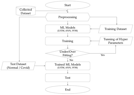
Figure 4.
Methodologies and modeling.
Four scenarios (A, B, C, and D) were devised and tested to analyze the effect of each selected variable on the model performance. Section 5, Section 6, Section 7 and Section 8 describe the analysis of each scenario.
- Scenario A: Application of a one-dimensional variable to verify the effectiveness of the ML models.
- Scenario B: Application of eight-dimensional variables to test the performance of ML models.
- Scenario C: Application of seven-dimensional variables to analyze the effect of JKM on the performance of the ML models.
- Scenario D: Application of two-dimensional variables to analyze the effect of each variable on model performance.
Table 4 summarizes the specifications of the environment and PC on which the spot LNG price prediction models were developed.
Table 4.
Data analytics environment.
5. Scenario A: Application of One-Dimensional Independent Variable
Section 5 presents an analysis of Scenario A to verify the effectiveness of ML models. Scenario A describes the application of a one-dimensional variable to the training and testing of the ML models. The predictive performances of the models were measured during normal and COVID-19 periods.
5.1. Training of ML Models
The preprocessed training dataset was used to train the developed ML models to predict the JKM and ARIMA models. First, the hyperparameters used to construct the ML model or minimize the loss function, such as the penalty parameter in SVM or the learning rate for ANN training, were optimized by iteratively training the ML models [67]. Three hyperparameters were adjusted for models using neural network-based algorithms such as LSTM and ANN: epoch, batch size, and learning rate. The developed prediction models were trained by iterating the same process based on the given variables. The number of iterations were determined by number (value) of epochs [68]. Next, the number of samples to be used in the network before updating the weights was set. The batch size setting determined the number of training samples used per epoch [68]. The learning rate indicated the rate at which the model parameters were adjusted for each batch and epoch [68]. Smaller learning rates result in slower training speeds, whereas larger learning rates may cause unpredictable behaviors during training. An inappropriate learning rate can cause the loss function value to fall below that of other existing solutions. Therefore, it is crucial to set a suitable initial value to update the learning rate [69]. Here, the authors tuned the hyperparameters using iterative model training based on the default values of each algorithm. Table 5 presents the final selected parameter values.
Table 5.
Hyper parameters of LSTM and ANN models.
The SVM algorithm-based model was developed using multi-SVR to incorporate multivariate independent variables. Since this model does not utilize epochs, there was no need to set that hyperparameter. However, it was necessary to determine the look-back and look-forward values, which are essential for predicting time series data. As the authors aimed to predict the JKM, spot LNG price, in the short term, they tested the predictive performance of the ML models for the next day, after five days, and after ten days. Therefore, the settings ‘look-back = 15′ and ‘look-forward = 1, 5, and 10′ were uniformly applied to the models.
The ARIMA model has a univariate variable structure; therefore, the JKM factor functions as both a dependent and independent variable in this model, making it unnecessary to divide the dataset into training, test, and COVID-19 test datasets, as was done for the ML models. However, to more intuitively compare ARIMA with the ML models, the authors identically split the dataset for the ARIMA model.
In Scenario A, reflecting the structural characteristics of the ARIMA model, whose performance was compared to that of the ML models for verification, only one JKM factor was applied as a univariate independent variable in the ML prediction models, after which training was conducted. Therefore, if the developed ML models show similar or higher capabilities than the ARIMA model’s verified performance, the soundness of the ML models can be verified. Furthermore, the criteria for assessing the influence of each variable used to train the ML models on prediction accuracy can be established.
5.2. Training Results
As a result of Scenario A training, all of the ML models produced performances similar to that of the ARIMA model. Nevertheless, for further predicted time points, the scores of the evaluation indicators increased, while the performance of the ML models decreased. A constant pattern of scores was recorded regardless of the ML model type. The ARIMA model showed an MAE of 0.014, MAPE of 0.046, and RMSE of 0.001, making it the best-performing model. However, the performance scores increased for further predicted time points. Table 6 and Figure 5 show the training evaluation indicator scores for each model.
Table 6.
The training results of scenario A.
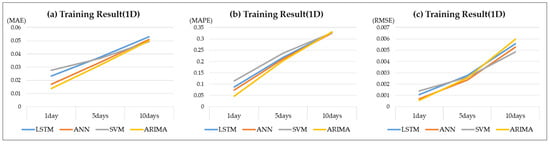
Figure 5.
The training results of scenario A. (a) MAE resulting from application of a one-dimensional variable. (b) MAPE resulting from application of a one-dimensional variable. (c) RMSE resulting from application of a one-dimensional variable.
5.3. Test and Validation
To evaluate the performance of each model, the authors used information collected over two years (2018–2019) to evaluate the normal period predictive accuracy of the ML algorithm-based prediction models trained by applying JKM as a one-dimensional independent variable. According to the test results, the ML models yielded prediction accuracies similar to those of the training results. Regarding the overall performance indicators MAE, MAPE, and RMSE, although the ML models slightly underperformed compared with the ARIMA model, their performance levels were nearly identical. The overall performance of the ML models was relatively weak; however, they outperformed the ARIMA model at certain time points and in some performance indicators. Notably, the performance indicator scores of both the ML and ARIMA models exhibited an almost constant pattern, thereby indicating that the performance according to the type of ML algorithm was nearly identical.
Through Scenario A testing, which involved using 15 days of previous JKM data as input, the authors confirmed that the performances of the ML models developed to predict JKM were nearly identical to that of the ARIMA model. This generated a new value for each time point and repeated the process of predicting values for 1, 5, and 10 days into the future. Therefore, theoretically, this structure inevitably derived predicted values that were nearly identical to actual values. Given that the developed ML prediction models produced similar performances to the ARIMA model, they can be judged as sound. Validating the soundness of the ML models is highly significant in this study, as this lays the foundation for conducting additional scenarios. The ARIMA model showed an MAE of 0.020, MAPE of 0.121, and RMSE of 0.001, making it the best-performing model. The performance scores increased for further predicted time points for both the ML and ARIMA models. Table 7 and Figure 6 show the performance indicator scores for each model.
Table 7.
The test results of scenario A.
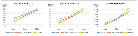
Figure 6.
The test results of scenario A. (a) MAE resulting from application of a one-dimensional variable. (b) MAPE resulting from application of a one-dimensional variable. (c) RMSE resulting from application of a one-dimensional variable.
5.4. Abnormal Period Analysis
The COVID-19 period data, which were prepared separately to compare the predictive power for the abnormal period, comprised two years of information (2020–2021), which were the same duration as the existing test dataset. The prepared COVID-19 data were used to perform the test. When measuring the predictive power for the abnormal period wherein market uncertainty was observed, the SVM model performed significantly better than the other models. Notwithstanding the accuracy of the predicted values, it failed to estimate the rising and falling trends of the actual values. In contrast, in the abnormal test, the performances of the neural network algorithm-based LSTM and ANN models were nearly identical to the normal test results. However, the prediction accuracy is likely to degrade for time points with sharply increasing prices. Table 8 and Figure 7 show the results of the abnormal (COVID-19, denoted as “COVID” in tables for simplicity) tests.
Table 8.
The COVID test results of scenario A.
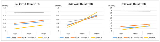
Figure 7.
The COVID test results of scenario A. (a) MAE resulting from application of a one-dimensional variable. (b) MAPE resulting from application of a one-dimensional variable. (c) RMSE resulting from application of a one-dimensional variable.
6. Scenario B: The Application of Eight-Dimensional Independent Variables
Section 6 describes the analysis of Scenario B to test the performance of the ML models. Scenario B is an application of eight-dimensional variables to the training and testing of the ML models. It measured the models’ predictive performances during normal and COVID-19 periods.
6.1. Training of ML Models
In Scenario A, the authors verified the soundness of the ML prediction models. The authors additionally analyzed the influence of the independent variables on the predictive performance of the ML models. In Scenario B, an eight-dimensional analysis was performed wherein the models were trained by applying JKM as a univariate independent variable and applying all the other seven variables.
6.2. Training Results
According to the model training results, the prediction accuracy of each ML model declined compared to those under Scenario A, although the disparity with Scenario A varied for each model. Moreover, in the Scenario B training results, the ML models underperformed compared with the ARIMA model, although the performance gap between the LSTM and SVM models and the ARIMA model decreased as the prediction period increased. Furthermore, the ML models outperformed the ARIMA model in some sections (10 d). A remarkable finding from the training results is that, compared with the other models, the SVM model exhibited consistent performance regardless of the predicted time point. Conversely, the ANN model output much lower predictive performance indicator scores than under Scenario A. Overall, the LSTM, ANN, and ARIMA models exhibited lower accuracy as the predicted time points increased. Among them, the LSTM model achieved an MAE of 0.040, MAPE of 0.157, and RMSE of 0.003, making it the best-performing model compared to the ARIMA model. It is important to note that the ARIMA model had the same analysis conditions; accordingly, the performance values are identical to those in Scenario A. Appendix A, Table A1 and Figure A1 show each model’s training scores by their evaluation indicators.
6.3. Test and Validation
Scenario B analysis was conducted by applying normal-period data to previously trained ML prediction models. According to the test results, the LSTM model produced the highest performance of the three ML models, followed in order by the ANN and SVM models. The SVM model showed stable performance regardless of the changes in the predicted time point. However, there was a large difference in the absolute prediction error compared with the other models, and its overall performance was the lowest. Furthermore, the ANN model produced lower performance for furthering predicted time points. The LSTM and ARIMA models exhibited relatively stable performances compared with the other models.
After applying the eight-dimensional variables, the MAE, MAPE, and RMSE scores, which are the performance indicators of each model, substantially increased compared with those under Scenario A, thereby indicating that the performance of all ML models decreased by a certain level. As the performance of the ML models declined, the gap in performance with the ARIMA model widened. Therefore, the seven additional variables applied in Scenario B negatively impacted the predictive performance of each ML model. Appendix A, Table A2, and Figure A2 show the evaluation indicator scores of each model calculated using the Scenario B test. For reference, the ARIMA model had the same analysis conditions; hence, the performance values were identical to those of Scenario A.
6.4. Abnormal Period Analysis
Upon comparing the predictive power of each model during the abnormal period, it was found that all models recorded relatively equal scores, regardless of the predicted time point. However, the absolute value of the prediction error differed in magnitude for each model. By analyzing the graphs of the predicted and actual values of each model, the authors confirmed that the prediction models had many practical limitations. Appendix A, Table A3, and Figure A3 show the performance indicator scores for each model during the abnormal period.
7. Scenario C: The Applications of 7 Dimensional Independent Variables
Section 7 presents an analysis of the effect of Scenario C on the JKM prediction performance of the ML models. Scenario C is an application of seven-dimensional variables to the training and testing of ML models. It measured the models’ predictive performances during normal and COVID-19 periods.
7.1. Training of ML Models
In Scenario C, seven variables were applied as multivariate independent variables to training the three ML models developed for the JKM prediction. Here, the JKM factor, which was applied as an independent variable in Scenarios A and B, was excluded from the variables.
7.2. Training Results
As a result of training, the ARIMA model produced the most accurate predictive performance, followed by the SVM and LSTM models. The ANN model showed the least accurate predictive results. The LSTM and SVM models showed relatively constant performance regardless of the predicted time point. Additionally, the performance of ANN and ARIMA model deteriorated as the prediction time point increased. The SVM showed an MAE of 0.082, MAPE of 0.204, and RMSE of 0.011, making it the best-performing model next to the ARIMA model. For reference, the ARIMA model had the same analysis conditions; thus, the performance values were identical to those under the previous scenarios. Appendix B, Table A4, and Figure A4 show the training results of each model.
7.3. Test and Validation
According to Scenario C testing, the LSTM model demonstrated the highest performance of the three ML models, followed in order by the ANN and SVM models. However, the ARIMA model achieved a substantially higher performance compared to the ML prediction models. Although the SVM and ARIMA models exhibited slightly lower performance for longer predicted time points, the accuracy of the ANN model notably improved for relatively distant predicted time points. The LSTM model showed an MAE of 0.395, MAPE of 3.323, and RMSE of 0.234, making it the best-performing model compared to the ARIMA model. For reference, the ARIMA model had the same analysis conditions, resulting in identical performance values as those in the previous scenarios. Appendix B, Table A5, and Figure A5 present the evaluation scores of each model.
7.4. Abnormal Period Analysis
The LSTM and ANN models exhibited nearly identical predictive performances for the abnormal period. Aside from outliers, where the market price spiked, the two models showed relatively accurate predictions of an upward price trend. However, the performance of the ANN model declined considerably compared with that in the normal period, making it difficult to identify upward or downward price trends. Based on the error between the predicted and actual values of each model, it was difficult to trust the predictive power of the ML models during the abnormal period. Appendix B, Table A6 and Figure A6 show the performance indicator scores of each ML model and the ARIMA model in the abnormal period.
8. Scenario D: Applications of Two-Dimensional Independent Variables
Section 8 presents an analysis of the effect of each variable on the models’ performances under Scenario D, which was an application of seven-dimensional variables to the training and testing of the ML models. It measured the models’ predictive performances during the normal and COVID-19 periods.
8.1. Training of ML Models
Based on the results of Scenario A, when JKM was applied as a univariate independent variable, the ML-based prediction models showed a similar performance to the ARIMA model. Furthermore, the results of Scenarios B and C demonstrated that applying multidimensional independent variables, including JKM, could sometimes degrade the performance of the ML models. Based on the analysis of the other scenarios results, in Scenario D, the authors analyzed each variable’s impact on JKM prediction. JKM, a univariate independent variable that produced the best performance, was applied as the basic training condition, whereas the other seven variables were applied one at a time to train the models. To efficiently conduct and analyze Scenario D, the authors conducted an analysis of the LSTM model, which exhibited the best average performance in Scenarios B and C. Table 9 summarizes each of the two-dimensional variable combinations used to train the LSTM model.
Table 9.
Combinations of variables.
8.2. Training Results
As a result of Scenario D training, the LSTM model exhibited very similar predictive performance for each two-dimensional variable combination, although there were differences for each variable. The LSTM model showed an MAE of 0.022, MAPE of 0.111, and RMSE of 0.001, making it the best-performing model compared to the ARIMA model. For reference, the ARIMA model had the same analysis conditions; therefore, the performance values were identical to those under the previous scenarios. Appendix C, Table A7, and Figure A7 show the evaluation indicator scores for each two-dimensional variable combination of the LSTM model.
8.3. Test and Validation
Based on the normal period testing, the LSTM model showed nearly identical performance, regardless of the two-dimensional variable combination. Of the variable combinations, the JKM model trained with JKM and Chinese LNG import volumes produced the lowest test performance, thereby showing a relatively large performance gap with the ARIMA model and LSTM model trainings with other two-dimensional variable combinations. This indicates that the Chinese LNG import volume had the least impact on JKM prediction. Meanwhile, the two-dimensional combinations of the remaining variables (NBP, Brent, and HH) showed nearly identical performances to that of the ARIMA model. However, the performance of the ARIMA model declined for further predicted time points. The LSTM model was relatively advantageous regarding the performance difference depending on the predicted time point. In the normal period, NBP had the greatest impact on JKM prediction, followed by Brent and HH. Appendix C, Table A8, and Figure A8 show the test results obtained by applying two-dimensional variables.
8.4. Abnormal Period Analysis
Based on the abnormal period test results, the performance of the ARIMA model was pre-eminent. Although the ARIMA model significantly outperformed the LSTM model in terms of short-term predictive power, its performance quickly declined over further predicted time points. This trend was more pronounced in the abnormal period. Meanwhile, the combination of the JKM and Brent variables, which produced high performance in the normal period, showed a marked performance decline in the COVID-19 test period. The NBP had the greatest impact on JKM prediction, followed in order by Japan’s LNG import volume and average temperature in Seoul. In conclusion, in Scenario D, the authors determined the priority of the variables that influenced the fluctuations in JKM spot LNG price. Appendix C, Table A9, and Figure A9 show the evaluation indicator scores for the abnormal period.
9. Conclusions
Section 9 summarizes the results of the research and reviews its practical applicability.
9.1. Summary
In this study, the authors developed prediction models using three ML algorithms (LSTM, ANN, and SVM) to predict JKM, which is a spot LNG price index. Furthermore, the authors validated the ML prediction models by comparing their performance with that of ARIMA, a traditional statistical prediction model. The authors varied the dimensions of independent variables applied to train the ML models, analyzed them under four scenarios, and measured the performance of each model. Based on the performance measurements of each ML model, although results differed based on each scenario’s application conditions and predicted time points, the LSTM algorithm-based model produced the best overall performance and was selected as the optimal model. Compared with other ML models, the LSTM model showed a balanced predictive performance and maintained a stable performance regardless of the predicted time point. While the LSTM model recorded similar MAE, MAPE, and RMSE scores to those of the ANN model, it was superior because it exhibited an overall balanced performance.
Regarding the characteristics of each algorithm, based on the training results, the neural-network-based LSTM and ANN models recorded relatively poor fitting scores compared with the SVM model. However, when test data were applied, they outperformed the SVM model and maintained a constant performance difference based on the predicted time point. In contrast, the regression-based SVM (multi-SVR) model produced excellent fitting results through iterative training. However, when the actual test dataset was applied, its overall performance declined significantly. This trend was observed in the analyses of all the scenarios. Furthermore, the SVM model’s predictive performance during the abnormal period was considerably lower than those of the LSTM and ANN models. In conclusion, the models applying neural network-based algorithms maintained constant performance even for a new dataset or abnormal period and had relatively strong performances. In contrast, the model that applied a regression-based algorithm showed large differences in performance for new data and the abnormal period, with high uncertainty owing to the inherent characteristics of the algorithm.
From the performance comparison between the ML models and the traditional statistical model, ARIMA, it was confirmed that the ARIMA model had considerably better predictive power. As shown in a graph of the ARIMA test results, there was almost no error between the predicted and actual values. The ARIMA model generated a new value for each time point based on the data for the previous 15 days of JKM, which was set as the prediction target, and predicted the values for 1, 5, and 10 days in the future. This is an intuitive result, considering the fundamental operating principle of the ARIMA model, which has a structure that is much closer to the concept of fitting than to that of prediction.
9.2. Discussion
The authors developed a JKM prediction model for the Spot LNG price index and derived an optimal algorithm through this research. The originality of the research topic can be highly evaluated as it set the Spot LNG price, which has never been adopted as a prediction target before. In addition, this research had three main distinctive features compared to previous studies. First, four models were developed to systematically analyze the impact of the independent variables used in the research process on the model’s prediction performance, and a total of 32 cases were analyzed. Second, the author developed multiple ML-based prediction models and not only derived the optimal model, but also verified the objectivity and limitations of the developed prediction model performance through performance comparisons with the traditional statistical ARIMA model. Third, the authors also aimed to compare and measure the performance of the developed model by classifying it before and after COVID-19, reflecting recent political and economic issues. This effort was made to reflect the current readership’s situation as much as possible by evaluating the prediction performance during a time of exceptional market volatility.
The practical application potential of the research results can be positively evaluated by the pure LNG buyers, who generally aim to procure volume to fill shortages calculated by forecasting demand. Because the spot LNG volume that LNG buyers must secure is usually fixed, they only consider when to purchase this volume. Determining the optimal purchase time and making prompt decisions have the most critical impact on the final purchased spot LNG price. Ultimately, the model would be highly applicable if it could accurately predict upward or downward price trends compared to the current point in time rather than accurately predicting future price levels. In practice, when making purchases, the absolute error between the predicted and actual values exhibited relatively low importance; hence, the models’ performances were reevaluated by estimating how accurately they predicted upward and downward trends.
The authors analyzed the test results of the LSTM model with eight-dimensional independent variables that produced the highest performance through a dichotomous accuracy test regarding rising or falling price trends. The model showed a prediction accuracy of approximately 53% and 57% for the normal and abnormal periods, respectively, indicating that the model maintained consistent trend prediction performance even for the abnormal period with uncertain market conditions. This level of performance was confirmed to be similar to that of Company A in Korea, which applied ML prediction to iron ore price forecasting and recorded a predictive accuracy of approximately 50–60%. However, because the absolute accuracy value was only slightly higher than 50%, the direct application of the model in practice had limitations. However, modifying and supplementing the model to improve its predictive performance increases its practical value; therefore, the implications of this study’s findings can be considered highly significant.
Based on the analysis results, the authors surveyed SMEs with at least ten years of experience in the LNG import/distribution business industry regarding current work practices and the model’s practical applicability. Practitioners in the LNG industry do not predict spot LNG prices. As discussed above, the forecasting accuracy is low because spot LNG prices are highly volatile. It is difficult to obtain work efficiency gains relative to the time spent forecasting the prices. However, changes in spot LNG prices are also qualitatively analyzed by considering current market conditions (each country’s LNG supply and demand conditions, nuclear plant operation rates, etc.), short-term climate change trends, and unexpected events in the LNG market. This analysis determines when to purchase spot LNG by accurately predicting the market trends. SMEs generally agree that this qualitative analysis does not consider market fluctuations, resulting in delayed purchasing decisions. The authors received positive responses that under these circumstances, an objective tool to quantitatively determine spot LNG price trends could be applied as a criterion to support spot LNG purchasing decisions. However, SMEs agreed with the precondition that it is necessary to increase trend prediction performance by improving and supplementing the ML prediction model developed in this study.
Considering the quantitative evaluation results obtained from the performance indicator scores of the ML models, it would be difficult to immediately apply the models to the LNG trading business in practice, given that the absolute value of the error between the actual and predicted values was significant. This can be interpreted as a limitation from the perspective of LNG traders, whose highest priority is to generate profit through market margins. The LNG traders seek to perform arbitrage through price differences between LNG distribution markets by securing spot LNG at competitive prices or price differences caused by cyclical demand patterns (climate and season). Therefore, the absolute prediction accuracy of the model is directly linked to profitability, making it challenging to apply the model in practice to price fluctuation risk reduction.
Several studies have been conducted to predict energy prices in situations where global uncertainty is maximized, such as the COVID pandemic and the subsequent Rus-sia–Ukraine conflict. In particular, various advanced techniques have been applied to investigate the impact of current situations on crude oil price volatility, including empirical mode decomposition (EMD) [70], geometric Brownian motion (GBM) [71], a mixture of GBM and a Poisson process [72], and a fractional integration method [73]. In the future, the development of energy price prediction systems, including those for crude oil and NG, is expected to incorporate not only the JKM prediction model proposed in this study but also the four methodologies mentioned earlier. These approaches are anticipated to be applicable for forecasting uncertainties, including extreme events.
9.3. Contributions
In recent years, many countries have considered environmental problems a vital issue. NG is recognized for its value as a bridge fuel in the transition from fossil fuels to renewable energy. Moreover, the recent conflict in Ukraine has highlighted the importance of NG in world energy security. Korea is the world’s third-largest LNG importer, importing approximately 45 million tons of LNG per year. This imported LNG is vaporized and supplied to power plants, industries, and households, and has been established as a major energy source for power generation and heating. In particular, Korea’s LNG power plants serve to reduce the peak demand. Therefore, accurately forecasting the demand and securing a stable NG supply is crucial. The most intuitive solution to satisfy the constantly fluctuating peak demand is to purchase spot LNG. However, our main concern is to help determine when to purchase spot LNG by predicting upward and downward price trends rather than accurately predicting the spot LNG price itself. Instead of focusing on price prediction accuracy when evaluating the developed ML model, supplementing this study to improve the model’s predictive power for rising or falling price trends can become a helpful tool for facilitating purchase decisions for spot LNG.
The quantitative forecasting tool of JKM can also contribute to government policy formulation. Although this study presents a forecasting model at a level that suggests the possibility of applying JKM forecasting in practice, it is important to note that if the accuracy of the JKM prediction model increases, it can enable timely response to the government’s natural gas demand through accurate international gas price predictions. Furthermore, it is expected to contribute to the government’s gas tariff policy formulation, which adheres to the price smoothing principle: the price determination rule for Korea’s urban gas.
10. Limitations and Further Works
Section 10 provides a thoughtful analysis of the limitations of this study and suggests future directions for improving the model’s performance. This study highlights several challenges in predicting the price of a specific good, such as spot LNG, which is a small component of a complex economic system comprising numerous factors with intricate interactions. Despite these challenges, this study has successfully identified limitations that can be addressed to improve the model’s performance.
The first limitation is the fundamental difficulty of predicting the spot LNG price due to the interactions of diverse economic, political, and physical variables. However, the findings of this study suggest that increasing the number of variables used for ML model training does not always lead to improved predictive performance. The second is the lack of background data to predict spot LNG prices, owing to the market’s closed nature and liquidity constraints. While the study has collected data spanning nearly ten years, the limited number of data points for each variable row ultimately impedes sufficient training of ML models, thereby degrading their performance. However, it is expected that as the spot LNG market matures and sufficient data is accumulated, the potential of the practical application will increase through the improved performance of the predictive models. The third limitation is the lack of uniform programming code for the ML models. Despite applying three different ML algorithms and modifying an overall programming code to complete model development, the authors encountered challenges in unifying the sophistication level and operating structure of all models used in the study, which affected the performance of each model. The fourth limitation is that this study did not apply advanced ML models or hybrid models combining different algorithms to maximize the strengths of each. In addition, the study did not construct a dynamic system to utilize the developed models continuously, which constitutes a fundamental limitation for practical applications. Finally, it is necessary to introduce the concept of continuously inflowing the latest data into the prediction model’s database in order to optimize the model developed in this study. Through this, it is expected that the predictive model will be able to actively conduct additional learning and improve its performance, thereby maximizing its utility.
In summary, while this study identified limitations in the model, it also suggested future directions for improving model performance and predicting the spot LNG price more accurately. With continued efforts to address these limitations, there is potential for significant progress in this field.
Author Contributions
Conceptualization, S.-F.Y., S.-W.C. and E.-B.L.; methodology, S.-F.Y. and S.-W.C.; software, S.-F.Y.; validation, S.-F.Y., S.-W.C. and E.-B.L.; formal analysis, S.-F.Y. and S.-W.C.; investigation, S.-F.Y. and S.-W.C.; resources, S.-F.Y. and E.-B.L.; data curation, S.-F.Y.; writing—original draft preparation, S.-F.Y.; writing—review and editing, S.-F.Y., S.-W.C. and E.-B.L.; visualization, S.-F.Y. and S.-W.C.; supervision, E.-B.L.; project administration, E.-B.L.; funding acquisition, S.-F.Y. and E.-B.L. All authors have read and agreed to the published version of the manuscript.
Funding
This study was carried out in 2022 as part of the natural gas supply project by the Korea Gas Corporation (KOGAS) for a stable and economical domestic natural gas supply in South Korea.
Institutional Review Board Statement
Not applicable.
Informed Consent Statement
Not applicable.
Data Availability Statement
Not applicable.
Acknowledgments
The authors would like to thank Sea-Eun Park (a Researcher at Pohang University of Science and Technology) for her academic and technical support to this study. The views expressed in this thesis/paper are solely those of the authors and do not represent those of any official organization or research sponsor.
Conflicts of Interest
The authors declare no conflict of interest.
Abbreviations
The following abbreviations and parameters are used in this paper:
| AI | Artificial Intelligence |
| ANN | Artificial Neural Network |
| CME | Chicago Mercantile Exchange |
| FOB | Free on Board |
| HH | Henry Hub |
| ICE | Intercontinental Exchange |
| ICP | Indonesian Crude Price |
| JCC | Japanese Custom Cleared Crude Oil |
| JKM | Japan Korea Marker |
| KDPS | KOGAS Data Package Systems |
| KMA | Korea Meteorological Administration |
| KOGAS | Korea Gas Corporation |
| LNG | Liquefied Natural Gas |
| LSTM | Long Short-Term Memory |
| MAE | Mean Absolute Error |
| MAPE | Mean Absolute Percentage Error |
| ML | Machine Learning |
| MMBtu | Metric Million British Thermal Unit |
| NBP | National Balancing Point |
| NG | Natural Gas |
| NYMEX | New York Mercantile Exchange |
| OTC | Over the Counter |
| PF | Project Financing |
| RMSE | Root Mean Squared Error |
| SME | Subject Matter Expert |
| SVM | Support Vector Machine |
| SVR | Support Vector Regression |
Appendix A. Scenario B
Table A1.
The training results of scenario B—details.
Table A1.
The training results of scenario B—details.
| Training Result | 1 Day | 5 Days | 10 Days | |||
|---|---|---|---|---|---|---|
| MAE | Rank | MAE | Rank | MAE | Rank | |
| LSTM | 0.040 | 2 | 0.043 | 2 | 0.058 | 3 |
| ANN | 0.051 | 3 | 0.066 | 4 | 0.079 | 4 |
| SVM | 0.055 | 4 | 0.057 | 3 | 0.058 | 2 |
| ARIMA | 0.014 | 1 | 0.032 | 1 | 0.050 | 1 |
| - | MAPE | Rank | MAPE | Rank | MAPE | Rank |
| LSTM | 0.157 | 3 | 0.198 | 1 | 0.214 | 2 |
| ANN | 0.149 | 2 | 0.207 | 4 | 0.265 | 3 |
| SVM | 0.187 | 4 | 0.207 | 3 | 0.188 | 1 |
| ARIMA | 0.046 | 1 | 0.204 | 2 | 0.330 | 4 |
| - | RMSE | Rank | RMSE | Rank | RMSE | Rank |
| LSTM | 0.003 | 2 | 0.003 | 2 | 0.006 | 2 |
| ANN | 0.004 | 4 | 0.007 | 4 | 0.010 | 4 |
| SVM | 0.004 | 3 | 0.004 | 3 | 0.004 | 1 |
| ARIMA | 0.001 | 1 | 0.003 | 1 | 0.006 | 3 |

Figure A1.
The training results of scenario B—graph. (a) MAE resulting from application of eight-dimensional variables. (b) MAPE resulting from application of eight-dimensional variables. (c) RMSE resulting from application of eight-dimensional variables.
Table A2.
The test results of scenario B—details.
Table A2.
The test results of scenario B—details.
| Test Result | 1 Day | 5 Days | 10 Days | |||
|---|---|---|---|---|---|---|
| MAE | Rank | MAE | Rank | MAE | Rank | |
| LSTM | 0.195 | 2 | 0.199 | 2 | 0.290 | 2 |
| ANN | 0.503 | 4 | 0.289 | 3 | 0.307 | 3 |
| SVM | 0.488 | 3 | 0.502 | 4 | 0.515 | 4 |
| ARIMA | 0.020 | 1 | 0.047 | 1 | 0.074 | 1 |
| - | MAPE | Rank | MAPE | Rank | MAPE | Rank |
| LSTM | 1.571 | 3 | 1.052 | 3 | 1.178 | 3 |
| ANN | 4.579 | 4 | 3.030 | 4 | 3.205 | 4 |
| SVM | 0.890 | 2 | 1.022 | 2 | 1.158 | 2 |
| ARIMA | 0.121 | 1 | 0.487 | 1 | 0.830 | 1 |
| - | RMSE | Rank | RMSE | Rank | RMSE | Rank |
| LSTM | 0.058 | 2 | 0.063 | 2 | 0.132 | 2 |
| ANN | 0.326 | 3 | 0.121 | 3 | 0.140 | 3 |
| SVM | 0.377 | 4 | 0.391 | 4 | 0.404 | 4 |
| ARIMA | 0.001 | 1 | 0.007 | 1 | 0.015 | 1 |

Figure A2.
The test results of scenario B—graph. (a) MAE resulting from application of eight-dimensional variables. (b) MAPE resulting from application of eight-dimensional variables. (c) RMSE resulting from application of eight-dimensional variables.
Table A3.
The COVID test results of scenario B—details.
Table A3.
The COVID test results of scenario B—details.
| COVID Result | 1 Day | 5 Days | 10 Days | |||
|---|---|---|---|---|---|---|
| MAE | Rank | MAE | Rank | MAE | Rank | |
| LSTM | 0.766 | 2 | 0.821 | 2 | 0.991 | 2 |
| ANN | 1.140 | 3 | 1.116 | 3 | 1.158 | 3 |
| SVM | 1.723 | 4 | 1.725 | 4 | 1.724 | 4 |
| ARIMA | 0.107 | 1 | 0.217 | 1 | 0.308 | 1 |
| - | MAPE | Rank | MAPE | Rank | MAPE | Rank |
| LSTM | 0.836 | 2 | 0.651 | 2 | 1.076 | 2 |
| ANN | 2.087 | 4 | 3.388 | 4 | 2.158 | 4 |
| SVM | 0.954 | 3 | 1.074 | 3 | 1.134 | 3 |
| ARIMA | 0.186 | 1 | 0.532 | 1 | 0.969 | 1 |
| - | RMSE | Rank | RMSE | Rank | RMSE | Rank |
| LSTM | 1.584 | 2 | 1.841 | 2 | 2.197 | 2 |
| ANN | 2.605 | 3 | 3.125 | 3 | 3.137 | 3 |
| SVM | 5.545 | 4 | 5.520 | 4 | 5.472 | 4 |
| ARIMA | 0.165 | 1 | 0.608 | 1 | 1.045 | 1 |

Figure A3.
The COVID test results of scenario B—graph. (a) MAE resulting from application of eight-dimensional variables. (b) MAPE resulting from application of eight-dimensional variables. (c) RMSE resulting from application of eight-dimensional variables.
Appendix B. Scenario C
Table A4.
The training results of scenario C—details.
Table A4.
The training results of scenario C—details.
| Training Result | 1 Day | 5 Days | 10 Days | |||
|---|---|---|---|---|---|---|
| MAE | Rank | MAE | Rank | MAE | Rank | |
| LSTM | 0.097 | 4 | 0.093 | 3 | 0.096 | 3 |
| ANN | 0.085 | 3 | 0.118 | 4 | 0.140 | 4 |
| SVM | 0.082 | 2 | 0.080 | 2 | 0.079 | 2 |
| ARIMA | 0.014 | 1 | 0.032 | 1 | 0.050 | 1 |
| - | MAPE | Rank | MAPE | Rank | MAPE | Rank |
| LSTM | 0.228 | 3 | 0.204 | 2 | 0.277 | 2 |
| ANN | 0.281 | 4 | 0.469 | 4 | 0.564 | 4 |
| SVM | 0.204 | 2 | 0.214 | 3 | 0.240 | 1 |
| ARIMA | 0.046 | 1 | 0.204 | 1 | 0.330 | 3 |
| - | RMSE | Rank | RMSE | Rank | RMSE | Rank |
| LSTM | 0.017 | 4 | 0.016 | 3 | 0.017 | 3 |
| ANN | 0.014 | 3 | 0.025 | 4 | 0.035 | 4 |
| SVM | 0.011 | 2 | 0.011 | 2 | 0.010 | 2 |
| ARIMA | 0.001 | 1 | 0.003 | 1 | 0.006 | 1 |

Figure A4.
The training results of scenario C—graph. (a) MAE resulting from application of seven-dimensional variables. (b) MAPE resulting from application of seven-dimensional variables. (c) RMSE resulting from application of seven-dimensional variables.
Table A5.
The test results of scenario C—details.
Table A5.
The test results of scenario C—details.
| Test Result | 1 Day | 5 Days | 10 Days | |||
|---|---|---|---|---|---|---|
| MAE | Rank | MAE | Rank | MAE | Rank | |
| LSTM | 0.395 | 2 | 0.394 | 2 | 0.486 | 3 |
| ANN | 0.600 | 3 | 0.468 | 3 | 0.483 | 2 |
| SVM | 0.619 | 4 | 0.614 | 4 | 0.615 | 4 |
| ARIMA | 0.020 | 1 | 0.047 | 1 | 0.074 | 1 |
| - | MAPE | Rank | MAPE | Rank | MAPE | Rank |
| LSTM | 3.323 | 3 | 1.836 | 2 | 1.866 | 2 |
| ANN | 8.403 | 4 | 5.373 | 4 | 4.986 | 4 |
| SVM | 3.128 | 2 | 3.132 | 3 | 3.047 | 3 |
| ARIMA | 0.121 | 1 | 0.487 | 1 | 0.830 | 1 |
| - | RMSE | Rank | RMSE | Rank | RMSE | Rank |
| LSTM | 0.234 | 2 | 0.247 | 2 | 0.334 | 3 |
| ANN | 0.479 | 3 | 0.278 | 3 | 0.321 | 2 |
| SVM | 0.530 | 4 | 0.522 | 4 | 0.526 | 4 |
| ARIMA | 0.001 | 1 | 0.007 | 1 | 0.015 | 1 |

Figure A5.
The test results of scenario C—graph. (a) MAE resulting from application of seven-dimensional variables. (b) MAPE resulting from application of seven-dimensional variables. (c) RMSE resulting from application of seven-dimensional variables.
Table A6.
The COVID test results of scenario C—details.
Table A6.
The COVID test results of scenario C—details.
| COVID Result | 1 Day | 5 Days | 10 Days | |||
|---|---|---|---|---|---|---|
| MAE | Rank | MAE | Rank | MAE | Rank | |
| LSTM | 1.080 | 2 | 1.099 | 2 | 1.166 | 2 |
| ANN | 1.199 | 3 | 1.105 | 3 | 1.239 | 3 |
| SVM | 1.759 | 4 | 1.756 | 4 | 1.756 | 4 |
| ARIMA | 0.107 | 1 | 0.217 | 1 | 0.308 | 1 |
| - | MAPE | Rank | MAPE | Rank | MAPE | Rank |
| LSTM | 1.179 | 2 | 1.560 | 3 | 0.924 | 1 |
| ANN | 5.146 | 4 | 2.697 | 4 | 2.106 | 4 |
| SVM | 1.481 | 3 | 1.469 | 2 | 1.526 | 3 |
| ARIMA | 0.186 | 1 | 0.532 | 1 | 0.969 | 2 |
| - | RMSE | Rank | RMSE | Rank | RMSE | Rank |
| LSTM | 2.769 | 2 | 2.870 | 2 | 2.682 | 2 |
| ANN | 2.981 | 3 | 3.047 | 3 | 3.292 | 3 |
| SVM | 5.618 | 4 | 5.599 | 4 | 5.544 | 4 |
| ARIMA | 0.165 | 1 | 0.608 | 1 | 1.045 | 1 |

Figure A6.
The COVID test results of scenario C—graph. (a) MAE resulting from application of seven-dimensional variables. (b) MAPE resulting from application of seven-dimensional variables. (c) RMSE resulting from application of seven-dimensional variables.
Appendix C. Scenario D
Table A7.
The training results of scenario D—details.
Table A7.
The training results of scenario D—details.
| Training Result | 1 Day | 5 Days | 10 Days | |||
|---|---|---|---|---|---|---|
| MAE | Rank | MAE | Rank | MAE | Rank | |
| LSTM 1 | 0.023 | 5 | 0.038 | 5 | 0.054 | 4 |
| LSTM 2 | 0.024 | 7 | 0.038 | 6 | 0.055 | 6 |
| LSTM 3 | 0.024 | 6 | 0.038 | 4 | 0.054 | 5 |
| LSTM 4 | 0.026 | 8 | 0.038 | 3 | 0.055 | 8 |
| LSTM 5 | 0.023 | 4 | 0.040 | 8 | 0.054 | 3 |
| LSTM 6 | 0.023 | 3 | 0.039 | 7 | 0.055 | 7 |
| LSTM 7 | 0.022 | 2 | 0.037 | 2 | 0.053 | 2 |
| ARIMA | 0.014 | 1 | 0.032 | 1 | 0.050 | 1 |
| - | MAPE | Rank | MAPE | Rank | MAPE | Rank |
| LSTM 1 | 0.117 | 7 | 0.228 | 7 | 0.328 | 6 |
| LSTM 2 | 0.116 | 6 | 0.217 | 3 | 0.325 | 5 |
| LSTM 3 | 0.139 | 8 | 0.235 | 8 | 0.348 | 8 |
| LSTM 4 | 0.106 | 3 | 0.219 | 5 | 0.316 | 3 |
| LSTM 5 | 0.088 | 2 | 0.216 | 2 | 0.300 | 1 |
| LSTM 6 | 0.116 | 5 | 0.217 | 4 | 0.319 | 4 |
| LSTM 7 | 0.111 | 4 | 0.225 | 6 | 0.313 | 2 |
| ARIMA | 0.046 | 1 | 0.204 | 1 | 0.330 | 7 |
| - | MAPE | Rank | MAPE | Rank | MAPE | Rank |
| LSTM 1 | 0.001 | 5 | 0.003 | 3 | 0.006 | 3 |
| LSTM 2 | 0.001 | 7 | 0.003 | 7 | 0.006 | 7 |
| LSTM 3 | 0.001 | 6 | 0.003 | 6 | 0.006 | 4 |
| LSTM 4 | 0.001 | 8 | 0.003 | 5 | 0.006 | 5 |
| LSTM 5 | 0.001 | 3 | 0.003 | 8 | 0.005 | 2 |
| LSTM 6 | 0.001 | 4 | 0.003 | 4 | 0.006 | 6 |
| LSTM 7 | 0.001 | 2 | 0.003 | 2 | 0.005 | 1 |
| ARIMA | 0.001 | 1 | 0.003 | 1 | 0.006 | 8 |

Figure A7.
The training results of scenario D—graph. (a) MAE resulting from application of two-dimensional variables. (b) MAPE resulting from application of two-dimensional variables. (c) RMSE resulting from application of two-dimensional variables.
Table A8.
The test results of scenario D—details.
Table A8.
The test results of scenario D—details.
| Test Result | 1 Day | 5 Days | 10 Days | |||
|---|---|---|---|---|---|---|
| MAE | Rank | MAE | Rank | MAE | Rank | |
| LSTM 1 | 0.039 | 6 | 0.060 | 5 | 0.083 | 6 |
| LSTM 2 | 0.038 | 5 | 0.060 | 4 | 0.082 | 4 |
| LSTM 3 | 0.046 | 7 | 0.063 | 7 | 0.085 | 7 |
| LSTM 4 | 0.077 | 8 | 0.125 | 8 | 0.181 | 8 |
| LSTM 5 | 0.036 | 4 | 0.062 | 6 | 0.080 | 3 |
| LSTM 6 | 0.035 | 3 | 0.059 | 3 | 0.083 | 5 |
| LSTM 7 | 0.034 | 2 | 0.057 | 2 | 0.080 | 2 |
| ARIMA | 0.020 | 1 | 0.047 | 1 | 0.074 | 1 |
| - | MAPE | Rank | MAPE | Rank | MAPE | Rank |
| LSTM 1 | 0.260 | 6 | 0.456 | 4 | 0.901 | 6 |
| LSTM 2 | 0.225 | 4 | 0.469 | 5 | 0.849 | 4 |
| LSTM 3 | 0.254 | 5 | 0.475 | 6 | 0.874 | 5 |
| LSTM 4 | 0.261 | 7 | 0.492 | 8 | 0.996 | 8 |
| LSTM 5 | 0.280 | 8 | 0.445 | 2 | 0.717 | 1 |
| LSTM 6 | 0.220 | 3 | 0.437 | 1 | 0.946 | 7 |
| LSTM 7 | 0.210 | 2 | 0.449 | 3 | 0.842 | 3 |
| ARIMA | 0.121 | 1 | 0.487 | 7 | 0.830 | 2 |
| - | RMSE | Rank | RMSE | Rank | RMSE | Rank |
| LSTM 1 | 0.003 | 6 | 0.007 | 4 | 0.013 | 4 |
| LSTM 2 | 0.003 | 5 | 0.007 | 3 | 0.013 | 3 |
| LSTM 3 | 0.004 | 7 | 0.007 | 7 | 0.014 | 6 |
| LSTM 4 | 0.010 | 8 | 0.024 | 8 | 0.049 | 8 |
| - | RMSE | Rank | RMSE | Rank | RMSE | Rank |
| LSTM 1 | 0.003 | 3 | 0.007 | 6 | 0.012 | 1 |
| LSTM 2 | 0.003 | 4 | 0.007 | 5 | 0.013 | 5 |
| LSTM 3 | 0.002 | 2 | 0.007 | 1 | 0.012 | 2 |
| LSTM 4 | 0.001 | 1 | 0.007 | 2 | 0.015 | 7 |

Figure A8.
The test results of scenario D—graph. (a) MAE resulting from application of two-dimensional variables. (b) MAPE resulting from application of two-dimensional variables. (c) RMSE resulting from application of two-dimensional variables.
Table A9.
The COVID test results of scenario D—details.
Table A9.
The COVID test results of scenario D—details.
| COVID Result | 1 Day | 5 Days | 10 Days | |||
|---|---|---|---|---|---|---|
| MAE | Rank | MAE | Rank | MAE | Rank | |
| LSTM 1 | 0.395 | 5 | 0.444 | 3 | 0.516 | 6 |
| LSTM 2 | 0.392 | 4 | 0.451 | 5 | 0.501 | 4 |
| LSTM 3 | 0.408 | 7 | 0.456 | 6 | 0.515 | 5 |
| LSTM 4 | 0.519 | 8 | 0.560 | 8 | 0.660 | 8 |
| LSTM 5 | 0.406 | 6 | 0.481 | 7 | 0.548 | 7 |
| LSTM 6 | 0.374 | 2 | 0.444 | 4 | 0.499 | 3 |
| LSTM 7 | 0.388 | 3 | 0.442 | 2 | 0.496 | 2 |
| ARIMA | 0.107 | 1 | 0.217 | 1 | 0.308 | 1 |
| - | MAPE | Rank | MAPE | Rank | MAPE | Rank |
| LSTM 1 | 0.278 | 4 | 0.537 | 4 | 0.772 | 4 |
| LSTM 2 | 0.282 | 5 | 0.527 | 2 | 0.742 | 3 |
| LSTM 3 | 0.301 | 7 | 0.560 | 7 | 0.862 | 6 |
| LSTM 4 | 0.326 | 8 | 0.468 | 1 | 0.647 | 1 |
| LSTM 5 | 0.256 | 2 | 0.591 | 8 | 0.937 | 7 |
| LSTM 6 | 0.284 | 6 | 0.542 | 6 | 0.808 | 5 |
| LSTM 7 | 0.259 | 3 | 0.538 | 5 | 0.734 | 2 |
| ARIMA | 0.186 | 1 | 0.532 | 3 | 0.969 | 8 |
| - | RMSE | Rank | RMSE | Rank | RMSE | Rank |
| LSTM 1 | 0.757 | 3 | 0.866 | 2 | 1.065 | 6 |
| LSTM 2 | 0.789 | 5 | 0.895 | 5 | 1.037 | 2 |
| LSTM 3 | 0.786 | 4 | 0.895 | 4 | 1.053 | 5 |
| LSTM 4 | 0.979 | 8 | 0.952 | 7 | 1.172 | 7 |
| LSTM 5 | 0.868 | 7 | 1.030 | 8 | 1.249 | 8 |
| LSTM 6 | 0.729 | 2 | 0.889 | 3 | 1.026 | 1 |
| LSTM 7 | 0.815 | 6 | 0.927 | 6 | 1.052 | 4 |
| ARIMA | 0.165 | 1 | 0.608 | 1 | 1.045 | 3 |

Figure A9.
The COVID test results of scenario D—graph. (a) MAE resulting from application of two-dimensional variables. (b) MAPE resulting from application of two-dimensional variables. (c) RMSE resulting from application of two-dimensional variables.
References
- Korea Gas Corporation. Natural Gas Extraction and Refining. Available online: https://www.kogas.or.kr:9450/site/koGas/1040301000000 (accessed on 30 November 2022).
- BP plc. Statistical Review of World Energy 2021: A Dramatic Impact on Energy Markets. Available online: https://www.bp.com/en/global/corporate/news-and-insights/press-releases/bp-statistical-review-of-world-energy-2021-a-dramatic-impact-on-energy-markets.html (accessed on 5 December 2022).
- Statista. Countries with Largest Liquefied Natural Gas (LNG) Export Capacity in Operation Worldwide as of July 2022. Available online: https://www.statista.com/statistics/1262074/global-lng-export-capacity-by-country/ (accessed on 13 February 2023).
- Raj, R.; Suman, R.; Ghandehariun, S.; Kumar, A.; Ticonflicti, M.K. A techno-economic assessment of the liquefied natural gas (LNG) production facilities in Western Canada. Sustain. Energy Technol. Assess. 2016, 18, 140–152. [Google Scholar] [CrossRef]
- Sorge, M. The Nature of Credit Risk in Project Finance. BIS Q. Rev. Dec. 2011. Available online: https://ssrn.com/abstract=1967464 (accessed on 7 December 2022).
- Bosma, P.; Nagelvoort, R.K. Liquefaction technology; developments through history. In Proceedings of the 1st Annual Gas Processing Symposium, Doha, Qatar, 10–12 January 2009; pp. 19–31. [Google Scholar]
- International Group of Liquefied Natural Gas Importers. GIIGNL 2022 Annual Report. Available online: https://giignl.org/document/giignl-2022-annual-report/ (accessed on 5 December 2022).
- Brogaard, J.; Ringgenberg, M.C.; Sovich, D. The economic impact of index investing. Rev. Financ. Stud. 2019, 32, 3461–3499. [Google Scholar] [CrossRef]
- National Gas. Gas Winter Outlook 2022/23. Available online: https://www.nationalgas.com/document/140921/download (accessed on 7 December 2022).
- Korea Energy Economics Institute. World Energy Market Insight. Available online: http://www.keei.re.kr/insight?open&p=%2Fweb_energy_new%2Finsight.nsf%2Finsight_list.html&s=%3Fopen%26menu%3Dinsight%26doctype%3D0%26region%3Dall (accessed on 17 November 2022).
- Xiong, P.; Li, K.; Shu, H.; Wang, J. Forecast of natural gas consumption in the Asia-Pacific region using a fractional-order incomplete gamma grey model. Energy 2021, 237, 121533. [Google Scholar] [CrossRef]
- Korea Economic Research Institute. Economy. Available online: http://www.keri.org/web/eng/economic-trends-and-outlook (accessed on 7 December 2022).
- S&P Global Inc. Platts JKM™ (Japan Korea Marker) LNG Price Assessment. Available online: https://www.spglobal.com/commodityinsights/en/our-methodology/price-assessments/lng/jkm-japan-korea-marker-gas-price-assessments (accessed on 6 December 2022).
- CME Group. Henry Hub Natural Gas. Available online: https://www.cmegroup.com/markets/energy/natural-gas/natural-gas.quotes.html (accessed on 13 December 2022).
- ICE. UK NBP Natural Gas Futures. Available online: https://www.ice.com/products/910/UK-Natural-Gas-Futures (accessed on 13 December 2022).
- S&P Global Commodity Insights. Platts LNG Daily. Available online: https://www.spglobal.com/commodityinsights/en/products-services/lng/lng-daily (accessed on 13 December 2022).
- Gao, S.; Lei, Y. A new approach for crude oil price prediction based on stream learning. Geosci. Front. 2017, 8, 183–187. [Google Scholar] [CrossRef]
- Su, M.; Zhang, Z.; Zhu, Y.; Zha, D.; Wen, W. Data driven natural gas spot price prediction models using machine learning methods. Energies 2019, 12, 1680. [Google Scholar] [CrossRef]
- Xian, L.J.; Ismail, S.; Mustapha, A.; Abd Wahab, M.H.; Idrus, S.Z.S. Crude oil price forecasting using hybrid support vector machine. In Proceedings of the IOP Conference Series: Materials Science and Engineering, Penang, Malaysia, 17–18 April 2020; p. 012045. [Google Scholar]
- Gupta, N.; Nigam, S. Crude oil price prediction using artificial neural network. Procedia Comput. Sci. 2020, 170, 642–647. [Google Scholar] [CrossRef]
- Seo, S.H. Forecasting Korean LNG Import Price Using ARIMAX, VECM, LSTM and Hybrid Models. Master’s Thesis, Graduate School of Technology and Innovation Management, Ulsan, Republic of Korea, 2021. [Google Scholar]
- Mouchtaris, D.; Sofianos, E.; Gogas, P.; Papadimitriou, T. Forecasting Natural Gas Spot Prices with Machine Learning. Energies 2021, 14, 5782. [Google Scholar] [CrossRef]
- Fetih, K.; BALKAYA, C. Artificial Intelligence in Crude Oil Price Forecasting. TAS J. 2021, 1, 14–24. [Google Scholar]
- Kaymak, Ö.Ö.; Kaymak, Y. Prediction of crude oil prices in COVID-19 outbreak using real data. Chaos Solitons Fractals 2022, 158, 111990. [Google Scholar] [CrossRef]
- Tschora, L.; Pierre, E.; Plantevit, M.; Robardet, C. Electricity price forecasting on the day-ahead market using machine learning. Appl. Energy 2022, 313, 118752. [Google Scholar] [CrossRef]
- Tan, Y.Q.; Shen, Y.X.; Yu, X.Y.; Lu, X. Day-ahead electricity price forecasting employing a novel hybrid frame of deep learning methods: A case study in NSW, Australia. Electr. Power Syst. Res. 2023, 220, 109300. [Google Scholar] [CrossRef]
- Qin, Q.; Huang, Z.; Zhou, Z.; Chen, C.; Liu, R. Crude oil price forecasting with machine learning and Google search data: An accuracy comparison of single-model versus multiple-model. Eng. Appl. Artif. Intell. 2023, 123, 106266. [Google Scholar] [CrossRef]
- Ramakrishnan, S.; Butt, S.; Chohan, M.A.; Ahmad, H. Forecasting Malaysian exchange rate using machine learning techniques based on commodities prices. In Proceedings of the 2017 International Conference on Research and Innovation in Information Systems (ICRIIS), Langkawi, Malaysia, 16–17 July 2017; pp. 1–5. [Google Scholar]
- Fu, S.; Li, Y.; Sun, S.; Li, H. Evolutionary support vector machine for RMB exchange rate forecasting. Phys. A Stat. Mech. Appl. 2019, 521, 692–704. [Google Scholar] [CrossRef]
- Vijh, M.; Chandola, D.; Tikkiwal, V.A.; Kumar, A. Stock closing price prediction using machine learning techniques. Procedia Comput. Sci. 2020, 167, 599–606. [Google Scholar] [CrossRef]
- Truong, Q.; Nguyen, M.; Dang, H.; Mei, B. Housing price prediction via improved machine learning techniques. Procedia Comput. Sci. 2020, 174, 433–442. [Google Scholar] [CrossRef]
- Kim, H.-M.; Bock, G.-W.; Lee, G. Predicting Ethereum prices with machine learning based on Blockchain information. Expert Syst. Appl. 2021, 184, 115480. [Google Scholar] [CrossRef]
- Choi, S.-W.; Lee, E.-B.; Kim, J.-H. The Engineering Machine-Learning Automation Platform (EMAP): A Big-Data-Driven AI Tool for Contractors’ Sustainable Management Solutions for Plant Projects. Sustainability 2021, 13, 10384. [Google Scholar] [CrossRef]
- Kurani, A.; Doshi, P.; Vakharia, A.; Shah, M. A comprehensive comparative study of artificial neural network (ANN) and support vector machines (SVM) on stock forecasting. Ann. Data Sci. 2021, 10, 183–208. [Google Scholar] [CrossRef]
- Chhajer, P.; Shah, M.; Kshirsagar, A. The applications of artificial neural networks, support vector machines, and long–short term memory for stock market prediction. Decis. Anal. J. 2022, 2, 100015. [Google Scholar] [CrossRef]
- Xiong, X.; Qing, G. A hybrid day-ahead electricity price forecasting framework based on time series. Energy 2023, 264, 126099. [Google Scholar] [CrossRef]
- Iftikhar, H.; Bibi, N.; Canas Rodrigues, P.; López-Gonzales, J.L. Multiple Novel Decomposition Techniques for Time Series Forecasting: Application to Monthly Forecasting of Electricity Consumption in Pakistan. Energies 2023, 16, 2579. [Google Scholar] [CrossRef]
- Gosasang, V.; Chandraprakaikul, W.; Kiattisin, S. A comparison of traditional and neural networks forecasting techniques for container throughput at Bangkok port. Asian J. Shipp. Logist. 2011, 27, 463–482. [Google Scholar] [CrossRef]
- Siami-Namini, S.; Namin, A.S. Forecasting economics and financial time series: ARIMA vs. LSTM. arXiv 2018, arXiv:1803.06386. [Google Scholar] [CrossRef]
- Makridakis, S.; Spiliotis, E.; Assimakopoulos, V. Statistical and Machine Learning forecasting methods: Concerns and ways forward. PLoS ONE 2018, 13, e0194889. [Google Scholar] [CrossRef] [PubMed]
- Sagheer, A.; Kotb, M. Time series forecasting of petroleum production using deep LSTM recurrent networks. Neurocomputing 2019, 323, 203–213. [Google Scholar] [CrossRef]
- Guo, J. Oil price forecast using deep learning and ARIMA. In Proceedings of the 2019 International Conference on Machine Learning, Big Data and Business Intelligence (MLBDBI), Taiyuan, China, 8–10 November 2019; pp. 241–247. [Google Scholar]
- Calkoen, F.; Luijendijk, A.; Rivero, C.R.; Kras, E.; Baart, F. Traditional vs. machine-learning methods for forecasting sandy shoreline evolution using historic satellite-derived shorelines. Remote Sens. 2021, 13, 934. [Google Scholar] [CrossRef]
- Poggi, A.; Di Persio, L.; Ehrhardt, M. Electricity Price Forecasting via Statistical and Deep Learning Approaches: The German Case. Appl. Math. 2023, 3, 316–342. [Google Scholar] [CrossRef]
- Korea Meteorological Administration. Open MET Data Portal. Available online: https://data.kma.go.kr/resources/html/en/aowdp.html (accessed on 18 January 2023).
- Zou, Q.; Yi, C.; Wang, K.; Yin, X.; Zhang, Y. Global LNG market: Supply-demand and economic analysis. IOP Conf. Ser. Earth Environ. Sci. 2022, 983, 012051. [Google Scholar] [CrossRef]
- Center on Global Energy Policy. Asian LNG Trading Hubs: Myth or Reality. Available online: https://www.energypolicy.columbia.edu/publications/asian-lng-trading-hubs-myth-or-reality (accessed on 18 January 2023).
- Korea Meteorological Administration. World Climate. Available online: https://www.kma.go.kr/eng/weather/climate/worldclimate.jsp (accessed on 13 December 2022).
- Yan, W.-L. Stock index futures price prediction using feature selection and deep learning. N. Am. J. Econ. Financ. 2023, 64, 101867. [Google Scholar] [CrossRef]
- Cai, J.; Luo, J.; Wang, S.; Yang, S. Feature selection in machine learning: A new perspective. Neurocomputing 2018, 300, 70–79. [Google Scholar] [CrossRef]
- García, S.; Luengo, J.; Herrera, F. Tutorial on practical tips of the most influential data preprocessing algorithms in data mining. Knowl.-Based Syst. 2016, 98, 1–29. [Google Scholar] [CrossRef]
- Moon, T.; Lee, J.W.; Son, J.E. Accurate Imputation of Greenhouse Environment Data for Data Integrity Utilizing Two-Dimensional Convolutional Neural Networks. Sensors 2021, 21, 2187. [Google Scholar] [CrossRef]
- Farhangfar, A.; Kurgan, L.A.; Pedrycz, W. A novel framework for imputation of missing values in databases. IEEE Trans. Syst. Man Cybern. Syst. 2007, 37, 692–709. [Google Scholar] [CrossRef]
- Donders, A.R.T.; Van Der Heijden, G.J.; Stijnen, T.; Moons, K.G. A gentle introduction to imputation of missing values. J. Clin. Epidemiol. 2006, 59, 1087–1091. [Google Scholar] [CrossRef] [PubMed]
- Brownlee, J. Long Short-Term Memory Networks with Python: Develop Sequence Prediction Models with Deep Learning; Machine Learning Mastery: San Juan, PR, USA, 2017. [Google Scholar]
- Brownlee, J. Data Preparation for Machine Learning: Data Cleaning, Feature Selection, and Data Transforms in Python; Machine Learning Mastery: San Juan, PR, USA, 2020. [Google Scholar]
- Hastie, T.; Tibshirani, R.; Friedman, J.H. The Elements of Statistical Learning: Data Mining, Inference, and Prediction; Springer: New York, NY, USA, 2009; Volume 2. [Google Scholar]
- Ding, J.G.; He, Y.H.C.; Kong, L.P.; Peng, W. Camber Prediction Based on Fusion Method with Mechanism Model and Machine Learning in Plate Rolling. ISIJ Int. 2021, 61, 2540–2551. [Google Scholar] [CrossRef]
- Tang, Y.; Song, Z.; Zhu, Y.; Yuan, H.; Hou, M.; Ji, J.; Tang, C.; Li, J. A survey on machine learning models for financial time series forecasting. Neurocomputing 2022, 512, 363–380. [Google Scholar] [CrossRef]
- Sherstinsky, A. Fundamentals of Recurrent Neural Network (RNN) and Long Short-Term Memory (LSTM) network. Phys. D Nonlinear Phenom. 2020, 404, 132306. [Google Scholar] [CrossRef]
- Hochreiter, S.; Schmidhuber, J. Long short-term memory. Neural Comput. 1997, 9, 1735–1780. [Google Scholar] [CrossRef]
- Veza, I.; Irianto; Panchal, H.; Paristiawan, P.A.; Idris, M.; Fattah, I.M.R.; Putra, N.R.; Silambarasan, R. Improved prediction accuracy of biomass heating value using proximate analysis with various ANN training algorithms. Results Eng. 2022, 16, 100688. [Google Scholar] [CrossRef]
- Duval, F. Artificial Neural Networks: Concepts, Tools and Techniques Explained for Absolute Beginners; Cre-ateSpace Independent Publishing Platform: Scotts Valley, CA, USA, 2018. [Google Scholar]
- Li, Y.; Huang, X.; Zhao, C.; Ding, P. A novel remaining useful life prediction method based on multi-support vector regression fusion and adaptive weight updating. ISA Trans. 2022, 131, 444–459. [Google Scholar] [CrossRef]
- Ernst, F.; Schweikard, A. Fundamentals of Machine Learning: Support Vector Machines Made Easy; UTB GmbH: Stuttgart, Germany, 2020. [Google Scholar]
- Salman, A.G.; Kanigoro, B. Visibility Forecasting Using Autoregressive Integrated Moving Average (ARIMA) Models. Procedia Comput. Sci. 2021, 179, 252–259. [Google Scholar] [CrossRef]
- Yang, L.; Shami, A. On hyperparameter optimization of machine learning algorithms: Theory and practice. Neurocomputing 2020, 415, 295–316. [Google Scholar] [CrossRef]
- Kuhn, M.; Johnson, K. Applied Predictive Modeling; Springer: Berlin/Heidelberg, Germany, 2018. [Google Scholar]
- Takase, T.; Oyama, S.; Kurihara, M. Effective neural network training with adaptive learning rate based on training loss. Neural Netw. 2018, 101, 68–78. [Google Scholar] [CrossRef] [PubMed]
- Zhang, X.; Yu, L.; Wang, S.; Lai, K.K. Estimating the impact of extreme events on crude oil price: An EMD-based event analysis method. Energy Econ. 2009, 31, 768–778. [Google Scholar] [CrossRef]
- Shen, Z. Optimal Oil-based Exotic Options Strategies Under the Background of War: An Empirical Study in the Context of the Russia-Ukraine Conflict. In Proceedings of the 2022 2nd International Conference on Enterprise Management and Economic Development (ICEMED 2022), Dalian, China, 27–29 May 2022; pp. 954–961. [Google Scholar] [CrossRef]
- Agaton, C.B. Will a Geopolitical Conflict Accelerate Energy Transition in Oil-Importing Countries? A Case Study of the Philippines from a Real Options Perspective. Resources 2022, 11, 59. [Google Scholar] [CrossRef]
- Monge, M.; Romero Rojo, M.F.; Gil-Alana, L.A. The impact of geopolitical risk on the behavior of oil prices and freight rates. Energy 2023, 269, 126779. [Google Scholar] [CrossRef]
Disclaimer/Publisher’s Note: The statements, opinions and data contained in all publications are solely those of the individual author(s) and contributor(s) and not of MDPI and/or the editor(s). MDPI and/or the editor(s) disclaim responsibility for any injury to people or property resulting from any ideas, methods, instructions or products referred to in the content. |
© 2023 by the authors. Licensee MDPI, Basel, Switzerland. This article is an open access article distributed under the terms and conditions of the Creative Commons Attribution (CC BY) license (https://creativecommons.org/licenses/by/4.0/).