Abstract
The conditions for the onset of dissipation thermal instability with temperature-dependent viscosity in the plane Couette flow of a Newtonian fluid are analyzed. The studied system consists of a horizontal fluid layer confined between an adiabatic (fixed) lower wall and an isothermal (moving) upper wall. Both the exponential and the linear fluidity models are considered in order to account for the thermodependency of the fluid’s viscosity. The linear stability analysis of the base solution with respect to arbitrarily oriented normal modes is carried out numerically by employing a shooting method. The most unstable disturbances are proven to be stationary longitudinal rolls, and their stability is governed by three dimensionless parameters: the viscous dissipation Rayleigh number, Prandtl number and a parameter that represents the variability of the viscosity with temperature. It is shown that the effect of the variation of the viscosity is to promote the stability of the base flow. As expected, the two viscosity models’ results diverge as the variability of the viscosity increases, and the exponential model is found to be more stable than the linear fluidity one. By considering the thermophysical properties of real fluids, it is shown that viscous dissipation thermal instability precedes hydrodynamic instability. An energy budget analysis is proposed to better understand both the stabilization effect of the thermal variability of the viscosity and differences with viscous dissipation hydrodynamic instability.
1. Introduction
The impact of temperature-dependent viscosity on the convective motion of Newtonian and non-Newtonian fluids has received widespread attention in the past due to its applications in many industrial and geophysical contexts. Studies on thermal convection usually consider a vertical thermal gradient, generated either by external heating imposed at the horizontal boundaries or by internal heating by a heat source inside the medium. Stengel et al. [1] theoretically and experimentally investigated convection in a horizontal fluid layer heated from below with no internal heat sources (i.e., Rayleigh–Bénard convection) in order to determine the influence of the temperature dependence of viscosity on critical conditions at the onset of convection and on the nature of the bifurcation to finite amplitude convection. The important parameters in this problem are the Rayleigh number , Prandtl number and the ratio c of viscosities corresponding to the temperatures of the upper and lower boundaries. By assuming an exponential viscosity variation, Stengel et al. [1] found that three regimes can be distinguished: (i) low viscosity ratio (), where the critical Rayleigh number is nearly constant; (ii) moderate viscosity ratio (), where increases; and (iii) large viscosity ratio (), where reaches a peak and then decreases. Moreover, through experimental evaluation of heat transfer by measuring the Nusselt number, Stengel et al. [1] observed a heat flux jump at the onset of convection when the viscosity ratio c exceeded 150, indicating that the bifurcation is subcritical. The recent paper by Solomatova and Jain [2] helps to understand subcritical convection in temperature-dependent viscosity fluids. The extension to non-Newtonian fluids of Rayleigh–Bénard convection with temperature-dependent viscosity was accomplished by Sekhar and Jayalatha [3] for viscoelastic fluids and by Darbouli et al. [4] and Varé et al. [5] for shear-thinning fluids. The linear stability performed in [3] showed a stabilizing effect of the variable viscosity and strain retardation time, while the stress relaxation parameter destabilized the system at the onset of convection. For shear-thinning fluids, Darbouli et al. [4] conducted an experimental investigation of the Rayleigh–Bénard convection of Xanthan gum aqueous solutions by using magnetic resonance imaging techniques. They found that the critical Rayleigh number is not modified by the shear-thinning character of the fluid, and the onset occurs with a hexagonal pattern when the Xanthan concentration is increased. According to [4], the nonlinear selection of hexagonal cells may be attributed to variations in physical properties with temperature. The secondary instability of shear-thinning Rayleigh–Bénard convection was studied in [5] by using a weakly nonlinear stability analysis. Varé et al. [5] focused on the stability of hexagonal patterns towards spatially uniform disturbances and long wavelength perturbations. It was shown that the amplitude stability domain shrinks with increasing shear-thinning effects and increases with increasing the viscosity ratio c, whereas for the phase stability domain, which confines the range of stable wave numbers, it was found that it is closed for low values of c and becomes open and asymmetric for moderate values of c.
On the other hand, convection in planetary interiors, whose viscosity is a strong function of temperature, is at least partially driven by different sources of internal heating. This problem was investigated by Jaina and Solomatov [6] by using a two-dimensional numerical simulation with exponential temperature-dependent viscosity in the presence of uniform internal heating. It was found that as the viscosity ratio increases, a high-viscosity stagnant lid develops at the upper surface, and convection occurs near the lower boundary. In contrast to the Rayleigh–Bénard problem, the bifurcation to two-dimensional patters is supercritical, independently of the viscosity ratio.
The above literature survey, which is not exhaustive, shows that the variation of viscosity with temperature in Newtonian and non-Newtonian fluids in convection problems may significantly change linear properties at the onset of instability, as well as nonlinear pattern selection. The above-mentioned theoretical and experimental studies did not take into account the viscous dissipation effect. However, when viscous dissipation is considered, friction may generate unstable temperature gradients within the flow. Viscous dissipation and its implications for magma flows were investigated by Costa and Macedonio [7]. These authors found that in magma flows with typical flow rates, viscous heating is responsible for the evolution from Poiseuille flow, with a uniform temperature distribution at the inlet, to plug flow, with a hotter layer near the walls. When the temperature gradients induced by viscous heating are very pronounced, local instabilities may occur, and the triggering of secondary flows is possible.
Parallel to thermal instability investigations, the influence of viscous heating on hydrodynamic instability has been studied in some physical systems, especially in Couette and Taylor–Couette flows. The plane Couette flow, a simple shear flow between two infinite parallel plates, is a widely studied problem in hydrodynamic stability. It is well known that this flow is stable to small disturbances for a Newtonian fluid with constant physical properties [8]. However, when viscous dissipation is considered, friction may generate unstable temperature gradients within the flow. Early investigations of the plane Couette flow [9,10,11,12,13] showed that when the viscosity is allowed to vary with temperature, the velocity profile is affected by the internal viscous heating, and the plane Couette flow may become unstable. On the other hand, the effect of viscous heating on the stability of Newtonian Taylor–Couette flow has received considerable attention through both theoretical and experimental studies. Linear stability analysis by Al-Mubaiyedh et al. [14] predicts a new mode of instability due to viscous heating for highly viscous and thermally sensitive fluids, even in the absence of buoyancy. Subsequent experiments by White and Muller [15] confirmed the presence of this new instability triggered by viscous heating.
Differently from the aforementioned works, in the present paper, we consider a situation where the energy and momentum equations are coupled not only by the viscous force through a temperature-dependent viscosity of the fluid but also by gravitational body force through thermal buoyancy. A number of recent studies on buoyancy-induced dissipation instabilities have been undertaken considering a constant viscosity (see [16] for a survey). Barletta and coworkers performed linear stability analyses of buoyancy-induced instability caused by viscous dissipation in plane Couette [17] and Poiseuille [18] flows. These authors found that longitudinal rolls are the preferred mode of convection, and the onset of instability is described through the viscous dissipation Rayleigh number and Prandtl number , where and are, respectively, the Gebhart number and the Péclet number. Requilé et al. [19] extended their analysis to the weakly nonlinear regime and conclude that subcritical bifurcations may occur depending on the values of and . These studies considered, as in the present work, an adiabatic lower wall and an isothermal upper wall. Requilé and coworkers [20] carried out a linear analysis of the so-called Rayleigh–Bénard-Couette case, where other than the internal heating due to viscous dissipation, an external temperature gradient is imposed through fixed temperature boundary conditions. They showed that viscous dissipation induces changes in the critical Rayleigh and wave numbers at the onset of convection of longitudinal rolls. Two distinct instability regimes were observed. For moderate , the linear instability properties are almost similar to Rayleigh–Bénard convection. When becomes large enough, the viscous dissipation mechanism induces a strong destabilization and may trigger instability even if heating is from above.
On the other hand, in highly viscous fluids, important temperature gradients are needed to trigger convection, and the variation in fluid viscosity with temperature may no longer be negligible. For this reason, Barletta and Nield [21] analyzed the interplay between the effects of a temperature-dependent viscosity and a temperature-dependent density (thermal buoyancy) on dissipation instabilities in the case of a fluid-saturated porous layer. To the authors knowledge, the analysis of both effects in a fluid layer without porous matrix is lacking. Therefore, the present analysis can be viewed as an extension of [21] to the fluid layer case, as well as an extension of [17] to the case of variable viscosity. The results of this study can help improve our understanding of the conditions under which convection of highly viscous fluids occurs, especially in geophysics configurations. This paper is organized as follows. In Section 2, we present the mathematical formulation of the problem and the viscosity laws adopted (namely linear and exponential fluidity models). The properties of the base solution and the range of the viscosity parameter are presented for real fluids with known thermophysical properties in Section 3. Linearized equations and a Squire transformation, which can be adopted in order to map three-dimensional oblique structures onto corresponding bidimensional transverse rolls, are presented in Section 4. Numerical results and stability diagrams are shown in Section 5, and relations to hydrodynamic instability and Rayleigh–Bénard convection with variable viscosity are discussed. An energy budget analysis is then carried out in Section 6, and its results highlight the opposing roles played by the variable viscosity terms in the energy and momentum equations. Finally, the main conclusions are presented in Section 7.
2. Mathematical Model
A Newtonian fluid layer having an infinite horizontal extent and thickness is considered. We use a Cartesian frame such that the -axis is vertical, and , are horizontal. The lower () fixed wall is impermeable and adiabatic, while the upper () wall is impermeable, isothermal and moves with a constant velocity along the -axis. Asterisks denote dimensional coordinates (), time , velocity , temperature and pressure . The physical properties of the fluid are assumed to be constant, except the dynamic viscosity, which is a function of temperature and the density in the buoyancy force term, according to the Oberbeck–Boussinesq approximation. Under these assumptions, and by taking viscous dissipation into account, the local mass, momentum and energy balance equations can be written as
where is the rate-of-strain tensor. The last term in the energy equation represents the power per unit volume generated by viscous dissipation. Furthermore, is the thermal conductivity, is the reference fluid density evaluated at the upper wall temperature , is the specific heat at constant volume, is the dynamic temperature-dependent viscosity, is the thermal expansion coefficient and g is the modulus of the gravitational acceleration. The boundary conditions are writen as
The ratio is called the fluidity function [9]. Two different models are used to express the temperature change in the fluid viscosity, i.e., the exponential fluidity model or Nahme model [22]
and the linear fluidity model [9,23]:
where is a positive constant and is the viscosity evaluated at . We note that the linear fluidity function can be considered as a first-order approximation of the exponential one, and it is therefore valid over a limited temperature range.
The governing equations are nondimensionalized using the following scales: for space, for time, for the velocity field, for pressure and for the temperature difference , where is the thermal diffusivity and the kinematic viscosity. The following dimensionless equations are obtained:
where and are the Gebhart and Prandtl numbers, respectively. The dimensionless boundary conditions are written as
where the Péclet number represents the throughflow intensity and is defined as . In dimensionless form, the two fluidity models (22) and (6) become
with as the dimensionless parameter which measures the sensitivity of the viscosity to temperature variations.
3. Base Flow and Range of Viscosity Parameter
3.1. Base Flow and Its Properties
We seek a stationary solution of system (7)–(10) such that the temperature field T and velocity component u depend only on z:
with the boundary conditions
For the exponential fluidity model, the exact analytical solution was derived by Gavis and Laurence [24]:
with .
For the linear fluidity model, we found the following after some calculations:
with .
Note that in the case of a constant viscosity (), , and reduce to
and in that case, depends only on the dimensionless number , which may be seen as a viscous dissipation Rayleigh number (see [25]).
Thermodependent viscosity introduces, in addition to , either the parameter V or the product , known in the literature as Nahme number , defined by
The Nahme number is extensively used to study the hydrodynamic stability of shear flows when viscous dissipation is considered and buoyancy forces are neglected. In the present problem, as the instability is of thermal nature, in the first step, we present the results by using the viscous dissipation Rayleigh number and the viscosity parameter V as control parameters. Afterwards, we reformulate the stability results by introducing the Nahme number for comparison purposes with the hydrodynamic stability of Couette flow.
While Equations (20) and (21) show that the basic velocity normalized by and the basic viscosity ratio depend only on the product , Equation (19) shows that the basic temperature depends also on the viscosity parameter V in addition to . Therefore, one can examine the influence on the spatial basic temperature profile of the variation of the parameter V for a fixed viscous dissipation Rayleigh number or, inversely, the influence of the variation of for a fixed V.
For a fixed value of viscous dissipation Rayleigh number , Figure 1a presents the basic temperature distribution normalized by obtained with the two fluidity models and different values of the product . As seen in this figure, internal heating due to viscous dissipation yields a nonlinear distribution of the base temperature, contrarily to its linear distribution observed in the classical Rayleigh–Bénard configuration, where a temperature difference is imposed on the external walls. Such nonlinear base temperature distribution is due to frictional heating and is also observed in the case of a constant viscosity (). Moreover, it is observed that the fluid layer is cooled as (i.e., V) increases. This means that the increasing variability of the viscosity with a fixed viscous dissipation intensity stabilizes the system. The discrepancies among the two fluidity models increase with and are negligible for .
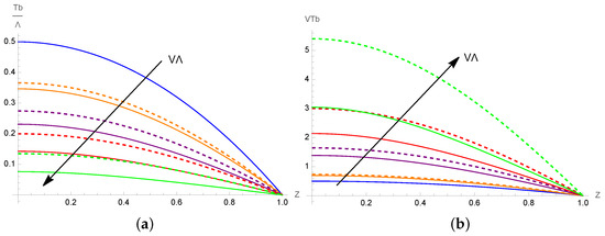
In the case of a fixed viscosity parameter V, the effect of (i.e., ) on the basic temperature profile is illustrated in Figure 1b. This figure shows that the fluid layer is heated more by increasing the viscous dissipation Rayleigh number , indicating the destabilizing effect of viscous dissipation. The plots of and are displayed in Figure 2a and Figure 2b, respectively. As it can be seen from Figure 2a, as increases from zero, the velocity profile loses its linearity and becomes more and more parabolic. Important discrepancies between the linear and exponential fluidity models are observed for . Figure 2b shows that as increases, large viscosity gradients appear near the upper boundary, while the fluid becomes less viscous near the lower boundary.
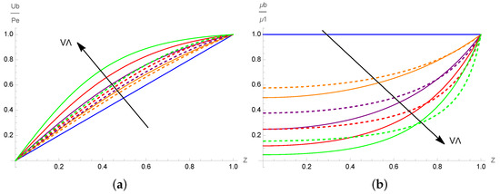
Figure 2.
Spatial distribution of (a) the basic velocity normalized by (Equation (20)) and (b) the basic viscosity normalized by the viscosity in the upper boundary (Equation (21)), obtained with the exponential (solid lines, Equation (11)) and linear (dashed lines, Equation (12)) fluidity models, for the same values of as in Figure 1.
3.2. Range of Variation in the Viscosity Parameter
Before performing a linear stability analysis of the basic state (19)–(21), it is instructive to evaluate the range of variation in the viscosity parameter in real liquids. Ali Amar et al. [25] examined the range of dimensional parameters needed to observe instabilities resulting from viscous dissipation in pure liquids, as well as in binary fluid mixtures with . It was found that one of the main constraints for the observability of such instability is that the height of the duct must exceed a minimum value, say of 1 cm. For , the physical quantities , , and for a given working fluid can be found in the literature or are measured in the laboratory. As significant and representative cases, we evaluate V for four liquids with moderate-to-high Prandtl numbers: water, mineral oil, natural ester and glycerol.
Nield [23] extended the classical Horton–Rogers–Lapwood problem (i.e., Rayleigh–Bénard convection in porous media) to the case where the viscosity of water varies with temperature. The linear stability analysis was conducted by assuming the linear fluidity model for water:
where is measured in and in C. Equation (23) states that
For fluids with an exponential viscosity variation, Stengel et al. [1] theoretically and experimentally investigated convection in a horizontal fluid layer with isothermal boundaries and no internal heat sources. With a cone–plate viscometer, these authors measured values of the dynamic viscosity of glycerol for a mean temperature ranging from to . The curve that fits all data may be approximated by an exponential viscosity variation with . On the other hand, the analysis of the thermal properties of natural ester and mineral oil was carried out by Dombek et al. [26] and Stanciu [27], respectively. The results fit exponential viscosity variation with for natural ester and for mineral oil. Table 1 presents the thermophysical properties and the corresponding values of the calculated viscosity parameter V for water, mineral oil, natural ester and glycerol, respectively. Table 1 indicates that for these representative liquids with Prandtl numbers ranging from to , the dimensionless parameter V is very small.

Table 1.
Values of the viscosity parameter V by fixing cm and expression of Nahme number determined by using models of thermodependent viscosity extracted, respectively, from ref. [23] for water, ref. [27] for mineral oil, ref. [26] for natural ester and ref. [1] for glycerol.
4. Linear Stability Analysis
Following the classical linear stability analysis procedure, we perturb the base solution with small-amplitude disturbances :
For the exponential fluidity model:
Additionally, for the linear fluidity model:
Using (19)–(27) and neglecting nonlinear terms, system (7)–(9) becomes
where the primes denote derivation with respect to z. The boundary conditions are given by
Solutions are sought in the form of normal modes
where and are the components of the wave vector, represents the temporal growth rate and is the oscillation frequency of the perturbation.
By substituting the normal modes into Equations (28)–(32), we obtain, at neutral stability conditions ():
where and . The boundary conditions become
4.1. Longitudinal Modes
For longitudinal rolls (LRs) having axes parallel to the base flow direction, we take . Then, we eliminate the pressure by cross-derivatives of Equations (35) and (37) and introduce the stream function :
By assuming that the principle of exchange of stability is valid, i.e., (such a hypothesis was verified on all the calculations performed in this work), the following set of linear perturbation equations for longitudinal modes is then obtained
where the x-component of the velocity is rescaled as , with . Note that for LRs, the Gebhart and Péclet numbers only appear in the combined form .
Boundary conditions are written as
It is useful to note that in the limit of infinite , the eigenvalue problem for longitudinal rolls is reduced to the following two equations
4.2. Squire Transformation
As in [17,25], for a general case without any approximation, Squire’s transformation cannot be applied to our problem. Nevertheless, it is shown in the following that for realistic cases where , the three-dimensional problem defined by system (34)–(38) can be Squire-transformed. By assuming , , as well as for realistic experimental setups with , which means that Equation (38) becomes
By setting in Equation (34), multiplying Equations (35) and (36) by and , respectively, and adding the result, the system (34)–(38) becomes (after replacing (38) by (46))
Comparing the formulations, one can easily reduce the three-dimensional problem to an equivalent two-dimensional problem by using the following transformation: , and .
Note that , and hence, at fixed and V, for every three-dimensional disturbance there exists a two-dimensional disturbance with the same threshold and the same frequency at a lower Péclet number given by the above transformation. Thus, in order to find the critical value at the onset of oblique rolls with an inclination angle for a fixed , it is sufficient to consider 2D transverse rolls and determine with instead of .
5. Results and Discussion
Equations (34)–(39) (or Equations (40)–(43) for LRs) form a generalized eigenvalue problem, which is solved for using a shooting method coded within the software Mathematica [28]. Details about this general shooting methodology can be found elsewhere [29]. The critical condition (, , ) is obtained by minimization of for the fixed values of , V and (or and V for LRs).
Viscous dissipation effects are the most significant when studying the stability of flows of highly viscous fluids. We therefore consider a highly viscous fluid with . It was verified that increasing the Prandtl number from this value leads to negligible differences in the stability results.
5.1. Three-Dimensional Versus Two-Dimensional Disturbances and Critical Thresholds
Figure 3a–c shows the neutral curves obtained for transverse rolls with three different values of the Péclet number at . In these figures, solid lines (dashed lines) correspond to neutral stability curves without (with) the approximation . The insets present zooms around critical conditions. As expected, the approximate solution becomes more accurate as increases. Furthermore, a comparison between the critical values in Figure 3a–c, obtained with , and , respectively, shows that the critical value decreases with the decrease in . As according to the Squire transformation, one may therefore conclude that for a fixed , the oblique rolls may develop at the onset of convection at a lower value of the viscous dissipation Rayleigh number (i.e more unstable) than the transverse rolls.
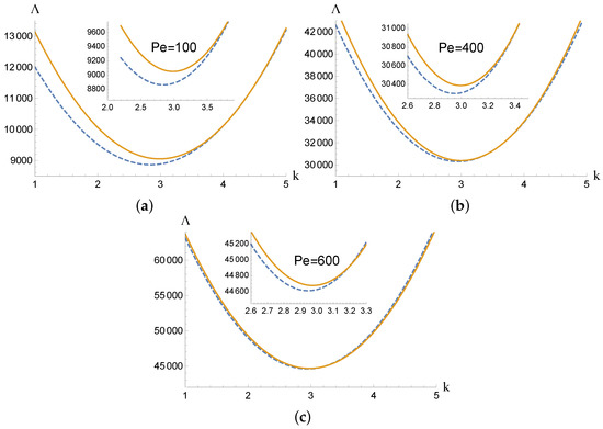
Figure 3.
Neutral curves obtained with the high approximation (dashed lines) and without it (solid lines) for , and (a) TRs with , (b) TRs with and (c) TRs with .
We first use the linear fluidity viscosity model to determine the dominant mode of instability. Figure 4a presents the stability diagram for transverse rolls, longitudinal rolls and oblique rolls with an inclination angle such that and . From Figure 4a, it can be observed that longitudinal rolls are the most unstable disturbances. The thresholds for the appearance of oblique structures lie well beyond the ones for longitudinal modes.
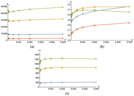
Figure 4.
Critical (a) , (b) and (c) as functions of parameter V, obtained with the linear fluidity model (Equation (12)) for stationary LR with (triangles), oscillatory oblique structures with (circles) and (squares) and oscillatory TRs with (diamonds).
Furthermore, longitudinal rolls are found to be stationary at the convection onset. All modes are slightly destabilized as V is increased from zero. After this small kink, the neutral curves in Figure 4a show a monotonic stabilization with increasing V. The evolution of the critical wave numbers and frequencies can be appreciated in Figure 4b,c. It can be noted that in the parameter range of the present study, the critical frequencies of oblique and transverse rolls seem to tend to an asymptotic value as V increases.
Let us now focus our attention on the properties of longitudinal rolls, which were also proven to be the most unstable disturbances in the constant viscosity case (the range of small Péclet numbers where the LRs are less unstable than oblique modes appears to be barely significant in practical situations [17]).
Table 2 presents the computed critical viscous dissipation Rayleigh number and critical wavenumber as a function of the viscosity parameter V, obtained with the exponential and linear fluidity models. Both models predict nearly constant and for ; otherwise, increasing V leads to an increase in and . This trend was expected given the base temperature profiles shown in Figure 1a. A very good agreement between the two viscosity models is obtained for very small values of V, as indicated by bold character in Table 2. For larger viscosity variability, the linear fluidity model tends to underestimate the critical and corresponding wave number . The effects of the Prandtl number were also investigated (not shown here). Negligible differences in the critical thresholds were observed when exceeded .
Table 2.
Critical and obtained with the linear (L) and exponential (E) fluidity models.
5.2. Relation to Hydrodynamic Instability and Rayleigh–Bénard Convection with Variable Viscosity
The stabilizing role of the thermal dependence of the viscosity was investigated in the previous sections by using the dimensionless parameter V. In order to make possible a comparison between the known results on hydrodynamic instability and Rayleigh–Bénard convection with variable viscosity, we need to reformulate the stability results in terms of the Nahme number defined by the relation (22) and viscosity ratio at the upper and lower boundaries ,
The stability diagrams in the () plane and in the () plane are, respectively, shown in Figure 5a,b.
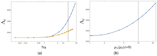
Figure 5.
Critical as a function of (a) Nahme number with exponential (circles, Equation (11)) and linear (squares, Equation (12)) fluidity models and (b) viscosity ratio , obtained with the exponential model. The vertical dashed line represents the border between the stable (left) and unstable (right) regions with respect to hydrodynamic instability.
It is important to examine the relevance of the stability results obtained in this paper by considering existing investigations of hydrodynamic viscous dissipation instability in Couette systems where buoyancy was neglected. The objective is to check whether the thermal instability studied here is established before or after the onset of hydrodynamic instability in Couette flow systems. Earlier investigations on the plane Couette flow with constant physical properties showed that this flow is linearly stable for a Newtonian fluid. A complete review can be found in the book by Drazin and Reid [8]. However, when the viscosity of fluids is assumed to depend on temperature, the plane Couette flow system may become unstable. In the case of thermodependent viscosity, the hydrodynamic stability problem is governed by both Reynolds number and Nahme number, defined by (22), which measures the viscous heating effect. In the inviscid limit (i.e., a flow with high Reynolds number), Joseph [9] used the linear fluidity–temperature model and showed that viscous heating may induce hydrodynamic instability. However, he did not consider the hydrodynamic instability properties at finite Reynolds numbers. Yueha and Weng [11] investigated the linear stability of a plane Couette flow of Newtonian fluids with finite Reynolds numbers by assuming exponential dependence of viscosity on temperature according to the Arrhenius law and Nahme law. Their results indicate that the plane Couette flow system exhibits two different modes of instability, an inviscid mode and a viscous mode, and the Arrhenius-type law was found to be more stable than the Nahme-type law. In [11], the authors used the Brinkman number, defined as , to compute the neutral stability curves in the (, ) plane with a fixed value of the viscosity parameter . It was found that the critical Reynolds number at the onset of the hydrodynamic instability increases when the Brinkman number decreases. More importantly, Yueha and Weng [11] found that the system is always stable when for all values of Reynolds number, which is the same as predicted by Joseph [9]. This result may be reformulated in terms of Nahme number by multiplying by , which is used in the computations of the eigenvalues in [11]. The result is that the hydrodynamic instability induced by viscous dissipation cannot be triggered for any Reynolds number provided that .
According to the above short review of hydrodynamic instability, the thermal viscous dissipation instabilities studied in the present work may or may not preceed hydrodynamic instability, depending on the Nahme number and critical Reynolds number. The dashed vertical lines in Figure 5a,b indicate a possible transition to hydrodynamic instability of Couette flows with variable viscosity when , or equivalently the viscosity ratio , exceed, respectively, or .
For different selected working fluids with known thermophysical properties and high , namely mineral oil, natural ester and glycerol, the determined values of and are reported in Table 3. As the values of the viscosity contrast parameter V and are documented in Table 1, we compute the corresponding critical viscous dissipation Rayleigh number at the onset of the instability, and therefore, the corresponding Nahme can be easily evaluated from the relationship .
Table 3.
Computed , and by fixing cm and using thermophysical properties extracted, respectively, from ref. [27] for mineral oil, ref. [26] for natural ester and ref. [1] for glycerol.
As seen in Table 3, the Nahme number and the viscosity ratio are, respectively, less than and 10 for these representative highly viscous Newtonian fluids. Moreover, it is very important to specify that the dimensional average velocity needed to trigger the hydrodynamic instability (i.e., ) is, respectively, m/s for mineral oil, m/s for natural ester and m/s for glycerol. These values of are too large and not physically realizable in laboratory experiments. We then conclude, according to the above discussion, that thermal instability due to viscous dissipation in Couette systems precedes the hydrodynamic instability for the three representative highly viscous fluids.
On the other hand, Stengel et al. [1] numerically and experimentally investigated the Rayleigh–Bénard convection by assuming different laws for the dependence of the viscosity on temperature. For exponential law, numerical results indicate that the behavior of the critical Rayleigh number and wavenumber depends on the viscosity ratio . Three regimes can be distinguished: (i) at low viscosity ratio ( ), the critical Rayleigh number is nearly constant; (ii) at viscosity ratio ( ), the critical Rayleigh number increases; and (iii) at large viscosity ratio ( ), the critical Rayleigh number reaches a peak and then decreases. A short inspection of Figure 5b attests that the critical viscous dissipation Rayleigh number remains nearly constant up to and then increases, including in the unphysical region of parameters where viscous dissipation hydrodynamic instability may develop.
6. Energy Budget Analysis
6.1. Thermal Energy Budget
An energy budget analysis is now carried out in order to better understand the physical mechanisms of the instability. Proceeding as in [20], the following relationship for the spatially averaged disturbance thermal energy is obtained:
with
where index r denotes the real part, constitutes the energy due to the thermal buoyancy contribution induced by viscous dissipation, corresponds to the hydrodynamic energy resulting from viscous dissipation, is the energy due to the contribution of the interaction between thermal dependence of the viscosity and viscous dissipation and corresponds to the thermal dissipation energy. The normalization of all the energy contributions allows to write the following at neutral conditions :
where , and .
The evolution of , and with V at can be appreciated in Figure 6a.
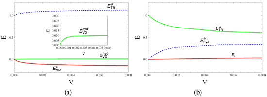
Figure 6.
Different energies versus V from the energy budget analysis of (a) thermal and (b) kinetic energy. The data were obtained using the linear fluidity model at .
It can be seen that the thermal buoyancy contribution is positive for all values of V, indicating its destabilizing effect. This destabilizing effect is accompanied by a negative (i.e., stabilizing) contribution of the variable viscosity contribution , while plays no significant role in this parameter range. We can conclude that the stabilization caused by the variable viscosity contribution is balanced by the increase in the thermal buoyancy contribution and therefore an increase in the critical viscous dissipation Rayleigh number with the viscosity parameter V, in agreement with the results of the linear modal stability analysis.
6.2. Kinetic Energy Budget
Although the stabilization effect of the thermodependence of viscosity was highlighted by the thermal energy budget analysis, we are also interested in the kinetic energy budget, with the hope of extracting some qualitative differences between thermal and hydrodynamic instabilities induced by viscous dissipation. The procedure is similar to the one used in [29], and we do not repeat it here. This procedure leads to the following relationship for the spatially averaged disturbance kinetic energy obtained:
with
where is the dissipation energy, corresponds to the contribution of the effect of thermodependence of the viscosity on viscous forces, is the thermal buoyancy contribution and is the contribution due to inertial forces. The different terms are normalized by the absolute value of the dissipation energy, and the onset of instability, we obtain:
with , and Plots of , and versus V are displayed in Figure 6a. One can note the small contribution of , which is slightly positive. It is seen from this figure that both and are positive, attesting the destabilizing role played by the two contributions. However, as the instability has a thermal origin, the destabilizing effect is more important for buoyancy forces than for viscous forces. In the case of purely hydrodynamic instability where buoyancy forces are neglected, it not surprising that the contribution of the thermodependence of viscosity to the viscous forces act in concert with inertia forces to destabilize the Couette system, as discussed previously.
It is interesting to note the opposite roles played by the variable viscosity in the Kinetic energy and thermal energy budgets. Whereas the viscous forces, due the changes in viscosity with temperature, promote destabilization in the kinetic budget, they play a stabilizing role in the thermal energy budget. As the present study focuses on thermal instabilities, the stabilizing role of thermal changes in viscosity in viscous dissipation terms of energy equation prevails, as shown in the previous sections.
7. Conclusions
A linear stability analysis was performed to investigate the combined influence of the viscous dissipation and temperature dependence of viscosity on the onset conditions of instability in Couette flow. The lower boundary of the plane channel is assumed to be thermally insulated, while the upper boundary is isothermal. Both linear and exponential fluidity laws are considered to model the thermodependence of the viscosity. A basic solution is composed by a negative nonlinear vertical temperature gradient and a spatially varying horizontal velocity and viscosity. Under the effect of increasing the temperature dependence of viscosity, the negative basic temperature gradient decreases, and the basic velocity profile becomes nonlinear. A stability analysis of this basic state against infinitesimal disturbances was carried out. A Squire transformation was proposed in order to map three-dimensional oblique structures onto corresponding two-dimensional transverse rolls. Therefore, by using the proposed Squire transformation, solving the eigenvalue problem numerically for arbitrarily oriented convective rolls is reduced to compute the eigenvalue problem for transverse rolls. As for the case of a constant viscosity, results indicate that the most unstable disturbances are stationary longitudinal rolls (). The linear characteristics of depend on the viscous dissipation Rayleigh number , Prandtl number and parameter V, which measures the viscosity variation with temperature. By considering four different types of Newtonian fluids, namely water (), mineral oil (), natural ester () and glycerol (), we show that the values of V, relevant for realistic laboratory experiments with the height of the channel fixed to cm, can hardly exceed . In this range of the parameter V, it was found that at the onset of convection, the critical viscous dissipation Rayleigh number and the corresponding critical wavenumber are nearly constant up to . When V exceeds , and increase, which means, respectively, that the thermodependence of the viscosity induces a stabilizing effect and reduces the width of the emerging rolls. The observed stabilization is more pronounced for the exponential fluidity model than for the linear one. For comparison purposes with hydrodynamic instability induced by viscous dissipation without buoyancy forces, we reformulated the stability results as a function of the Nahme number. It was shown that the thermal viscous dissipation instability with varying viscosity may develop at a Nahme number smaller than the one needed for the onset of the hydrodynamic instability. This result means that the thermal instability studied in the present work may be effective for viscous fluids. Finally, the stabilization effect of the thermodependence of viscosity is highlighted by a thermal energy budget analysis, while the kinetic energy budget analysis identified some qualitative differences between thermal and hydrodynamic instabilities induced by viscous dissipation.
Finally, we emphasize that if the viscous dissipation with temperature-dependent viscosity is an important factor to understand convection in geophysics flows, it also has practical interest in the polymer industry. Polymer solutions in viscous solvents are commonly used in the extrusion process, solidification of liquid crystals, petroleum activities and food production. These fluids are strongly viscous with a high Prandtl number and therefore are good candidates to develop viscous dissipation instability. The approach developed in the present study can be applied to explore the impact of viscous dissipation with temperature-dependent viscosity in viscoelastic fluids. This is the subject of a further work which is in preparation.
Author Contributions
Conceptualization, M.N.O. and S.C.H.; Methodology, M.N.O.; Software, A.S. and S.B.S.; Validation, A.S.; Formal analysis, M.N.O.; Investigation, A.S. and S.C.H.; Writing—original draft, S.C.H.; Writing—review & editing, M.N.O.; Supervision, S.C.H. and M.N.O. All authors have read and agreed to the published version of the manuscript.
Funding
This research was funded by Unité de Mécanique de Lille, URL 7512, Université de Lille.
Data Availability Statement
Not applicable.
Conflicts of Interest
The authors declare no conflict of interest.
References
- Stengel, K.C.; Oliver, D.S.; Booker, J.R. Onset of convection in a variable-viscosity fluid. J. Fluid Mech. 1982, 120, 411–431. [Google Scholar] [CrossRef]
- Solomatov, V.S.; Jain, C. Rayleigh–Bénard convection in temperature-dependent viscosity fluids: Constraints from two-dimensional simulations. Phys. Fluids 2021, 33, 056603. [Google Scholar] [CrossRef]
- Sekhar, G.N.; Jayalatha, G. Elastic effects on Rayleigh-Bénard convection in liquids with temperature-dependent viscosity. Int. J. Thermal Sci. 2010, 49, 67–75. [Google Scholar] [CrossRef]
- Darbouli, M.; Métivier, C.; Leclerc, S.; Nouar, C.; Bouteera, M.; Stemmelen, D. Natural convection in shear-thinning fluids: Experimental investigations by MRI. Int. J. Heat Mass Transf. 2016, 95, 742–754. [Google Scholar] [CrossRef]
- Varé, T.; Nouar, C.; Mxextivier, C.; Bouteraa, M. Stability of hexagonal pattern in Rayleigh-Benard convection for thermodependent shear-thinning fluids. J. Fluid Mech. 2020, 905, A33. [Google Scholar] [CrossRef]
- Jain, C.; Solomatov, V.S. Onset of convection in internally heated fluids with strongly temperature-dependent viscosity. Phys. Fluids 2022, 34, 096604. [Google Scholar] [CrossRef]
- Costa, A.; Macedonio, G. Viscous heating in fluids with temperature-dependent viscosity: Implications for magma flows. Nonlinear Process. Geophys. 2003, 10, 545–555. [Google Scholar] [CrossRef]
- Drazin, P.G.; Reid, W.H. Hydrodynamic Stability; University of Chicago: Chicago, IL, USA, 1981; p. 536. [Google Scholar]
- Joseph, D.D. Stability of frictionally-heated flow. Phys. Fluids 1965, 12, 2195–2200. [Google Scholar] [CrossRef]
- Sukanek, P.C.; Goldstein, C.A.; Laurence, R.L. Linear stability analysis of plane Couette flow with viscous heating. J. Fluid Mech. 1973, 4, 651–670. [Google Scholar] [CrossRef]
- Yueh, C.S.; Weng, C.L. The stability of plane Couette flow with viscous heating. J. Fluid Mech. 1996, 7, 1802–1813. [Google Scholar]
- Johns, L.E.; Narayanan, R. Frictional heating in plane Couette flow. Math. Phys. Eng. Sci. 1997, 1963, 1653–1670. [Google Scholar] [CrossRef]
- Subrahmaniam, N.; Johns, L.E.; Narayanan, R. Stability of frictional heating in plane Couette flow at fixed power input. Math. Phys. Eng. Sci. 2002, 2027, 2561–2569. [Google Scholar] [CrossRef]
- Al-Mubaiyedh, U.A.; Sureshkumar, R.; Khomami, B. Effect of viscous heating on the stability of Taylor–Couette flow. J. Fluids Mech. Fluids 2002, 462, 111. [Google Scholar] [CrossRef]
- White, J.M.; Muller, S.J. Experimental studies on the stability of Newtonian Taylor–Couette flow in the presence of viscous heating. J. Fluids Mech. Fluids 2002, 462, 133. [Google Scholar] [CrossRef]
- Barletta, A. On the thermal instability induced by viscous dissipation. Int. J. Therm. Sci. 2015, 88, 238–247. [Google Scholar] [CrossRef]
- Barletta, A.; Nield, D.A. Convection-dissipation instability in the horizontal plane Couette flow of a highly viscous fluid. J. Fluids Mech. 2010, 662, 475–492. [Google Scholar] [CrossRef]
- Barletta, A.; Celli, M.; Nield, D.A. On the onset of dissipation thermal instability for the Poiseuille flow of a highly viscous fluid in a horizontal channel. J. Fluids Mech. 2011, 681, 499–514. [Google Scholar] [CrossRef]
- Requilé, Y.; Hirata, S.C.; Ouarzazi, M.N.; Barletta, A. Weakly nonlinear analysis of viscous dissipation thermal instability in plane Poiseuille and plane Couette flows. J. Fluids Mech. 2020, 886, 1–21. [Google Scholar] [CrossRef]
- Requilé, Y.; Hirata, S.C.; Ouarzazi, M.N.; Barletta, A. Viscous dissipation effects on the linear stability of Rayleigh-Benard-Poiseuille/Couette convection. Int. J. Heat Mass Transf. 2020, 146, 1–11. [Google Scholar] [CrossRef]
- Barletta, A.; Nield, D.A. Variable viscosity effects on the dissipation instability in a porous layer with horizontal throughflow. Phys. Fluids 2012, 10, 1–18. [Google Scholar] [CrossRef]
- Nahme, R. Beitrage zur hydrodynamischen theorie der lagerreibung. Ing. Arch. 1940, 3, 191–209. [Google Scholar] [CrossRef]
- Nield, D.A. The Effect of Temperature- Dependent Viscosity on the Onset of Convection in a Saturated Porous Medium. J. Heat Transf. 1996, 118, 803–805. [Google Scholar] [CrossRef]
- Gavis, J.; Laurence, R.L. Viscous heating in plane and circular flow between moving surfaces. IEC Fundam. 1968, 7, 232–237. [Google Scholar] [CrossRef]
- Amar, K.A.; Hirata, S.C.; Ouarzazi, M.N. Soret effect on the onset of viscous dissipation thermal instability for Poiseuille flows in binary mixtures. Phys. Fluids 2022, 34, 114101. [Google Scholar] [CrossRef]
- Dombek, G. Thermal properties of natural ester and low viscosity natural ester in the aspect of the reliable operation of the transformer cooling system. Eksploat. I Niezawodn. Maint. Reliab. 2019, 21, 384–391. [Google Scholar] [CrossRef]
- Stanciu, I. A new viscosity-temperature relationship for mineral oil SAE 10W. Ovidius Univ. Ann. Chem. 2012, 23, 27–30. [Google Scholar] [CrossRef]
- Wolfram, S. Mathematica, version 9.0 Edition; Wolfram Research, Inc.: Champaign, IL, USA, 2013. [Google Scholar]
- Hirata, S.C.; Alves, L.S.B.; Delenda, N.; Ouarzazi, M.N. Convective and absolute instabilities in Rayleigh-Bénard-Poiseuille mixed convection for viscoelastic fluids. J. Fluids Mech. 2015, 765, 167–210. [Google Scholar] [CrossRef]
Disclaimer/Publisher’s Note: The statements, opinions and data contained in all publications are solely those of the individual author(s) and contributor(s) and not of MDPI and/or the editor(s). MDPI and/or the editor(s) disclaim responsibility for any injury to people or property resulting from any ideas, methods, instructions or products referred to in the content. |
© 2023 by the authors. Licensee MDPI, Basel, Switzerland. This article is an open access article distributed under the terms and conditions of the Creative Commons Attribution (CC BY) license (https://creativecommons.org/licenses/by/4.0/).