Article

An Enhanced Path Planner for Electric Vehicles Considering User-Defined Time Windows and Preferences

by
Maximiliano Cubillos
1,*,
Mauro Dell’Amico
2,
Ola Jabali
1,
Federico Malucelli
1 and
Emanuele Tresoldi
3
1
Dipartimento di Elettronica, Informazione e Bioingegneria, Politecnico di Milano, Piazza Leonardo da Vinci 32, 20133 Milano, Italy
2
Department of Sciences and Methods for Engineering, University of Modena and Reggio Emilia, Via Amendola 2, 42122 Reggio Emilia, Italy
3
Dipartimento di Informatica, Università degli Studi di Milano, Via Celoria 18, 20133 Milano, Italy
*
Author to whom correspondence should be addressed.
Energies 2023, 16(10), 4173; https://doi.org/10.3390/en16104173
Submission received: 18 April 2023 / Revised: 15 May 2023 / Accepted: 16 May 2023 / Published: 18 May 2023

Abstract

:
A number of decision support tools facilitating the use of Electric Vehicles (EVs) have been recently developed. Due to the EVs’ limited autonomy, routing and path planning are the main challenges treated in such tools. Specifically, determining at which Charging Stations (CSs) to stop, and how much the EV should charge at them is complex. This complexity is further compounded by the fact that charging times depend on the CS technology, the EV characteristics, and follow a nonlinear function. Considering these factors, we propose a path-planning methodology for EVs with user preferences, where charging is performed at public CSs. To achieve this, we introduce the Electric Vehicle Shortest Path Problem with time windows and user preferences (EVSPPWP) and propose an efficient heuristic algorithm for it. Given an origin and a destination, the algorithm prioritizes CSs close to Points of Interest (POIs) that match user inputted preferences, and user-defined time windows are considered for activities such as lunch and spending the night at hotels. The algorithm produces flexible solutions by considering clusters of charging points (CPs) as separate CSs. Furthermore, the algorithm yields resilient paths by ensuring that recommended paths have a minimum number of CSs in their vicinity. The main contributions of our methodology are the following: modeling user-defined time windows, including user-defined weights for different POI categories, creating CSs based on clusters of CPs with sufficient proximity, using resilient paths, and proposing an efficient algorithm for solving the EVSPPWP. To facilitate the use of our methodology, the algorithm was integrated into a web interface. We demonstrate the use of the web interface, giving usage examples and comparing different settings.

1. Introduction

Electric vehicle (EV) sales have significantly grown in the recent years. In Europe, for example, EV registrations have tripled from 3.5% in 2019 to 11.6% in 2020. This includes a 6.2% increase in fully electric vehicles [1]. Indeed, EVs are perceived to be a sustainable alternative to traditional combustion engine vehicles, offering advantages in terms of performance and reduced emissions [2]. However, a number of barriers impede a wider EV uptake. These include high purchase costs, limited autonomy, scarce charging infrastructure and lengthy charging times. To counter some of these barriers, an increasing number of decision support tools facilitating the use of EVs are being deployed. Such tools mainly rely on optimizing operational issues related EVs. In this vein, several contributions from the transportation science community have developed models and solution methods to EV routing problems (see Kucukoglu et al. [3] and Froger et al. [4] for examples).
We propose a methodology for planning EV paths considering user preferences, where charging is performed at public Charging Stations (CSs). The need for such a methodology for private EV users was identified through the eCharge4Drivers project, which is funded by the European Union Horizon 2020 programme. The proposed methodology was integrated in a web interface enabling a large audience to use it. The core optimization problem we deal with relates to planning the shortest path (in terms of time) for an EV needing to travel between a given origin and a given destination. This problem is particularly relevant for long-distance trips, where the shortest path between the origin and the destination exceeds the EV’s autonomy. The key decisions to be made in such problems are where to charge and how much to charge. The latter entails an amount of time which depends on the CS technology, the EV characteristics and follows a non-linear function. Moreover, as the charging infrastructure in road networks outside cities is fairly sparse, EVs often need to deviate from their shortest paths to reach CSs. The intertwined relationship between the time spent in detouring and the time spent charging is the main complicating feature of the Electric Vehicle Shortest Path Problem (EVSPP).
As EV charging times may take several hours, users (i.e., drivers) may prefer having charging stops at locations that match their interests. We consider that such interests may be captured via Points of Interests (POIs) that include categories such as restaurants, shopping areas, and nature sites. Moreover, we also consider that the user may want to perform some particular activity during specific time windows, like having lunch or spending the night at a hotel. Such user-defined time windows are also matched with relevant POIs locations. Thus, our overarching goal is to propose an efficient offline methodology integrating user preferences for POIs and user-specific time window into an EVSSP setting. To do so, we introduce the Electric Vehicle Shortest Path Problem with time windows and user preferences (EVSPPWP).
We model the EVSPPWP and propose an efficient heuristic algorithm to solve it. In particular, the algorithm prioritizes CSs that are close to POIs matching the user preferences. Furthermore, while we provide planned (offline) paths, we propose a number of algorithmic enhancements aimed at producing solutions that are practically executable in real time on large road networks. Specifically, the algorithm provides the user with robust and flexible solutions. To incorporate robustness, we only consider paths that have at least a given number CSs in their vicinity. This ensures that the EV could always reach a CS, in case its predicted energy consumption does not match the actual one. Additionally, it may occur that the EV encounters an occupied CS, which was planned in its path. To counter such situations, our algorithm produces flexible solutions by considering a CS as a cluster of charging points (CPs). While previous studies have used clustering for districting to reduce problem sizes in EVRPs [5], we focus on providing solutions so that users can find alternative CPs in cases where selected CPs are not available. Specifically, we produce small sized clusters of CPs that we treat as separate CSs. We plan the path based on those CSs. This entails having a number of CPs in the vicinity of a planned charging stop. Thus, if a CP is busy upon arrival, the user would have multiple alternatives in its vicinity.
Considering the previously discussed enhancements, we develop a heuristic algorithm for the EVSPPWP. We first include weights for each CS according to its vicinity to POIs that match the user-defined preferences. We then use a modified A * algorithm to establish the nodes where the user-defined time windows are going to be performed. Considering these nodes along with the user-defined origin and destination, we sequentially solve a series of modified EVSPPs (using the algorithm of Kullman et al. [6]), which we then aggregate into a complete solution. Lastly, the algorithm provides up to three alternative paths in a web interface where the users can visualize the path details.
To summarize, the main contributions of this papers are as follows.
  • We incorporate time windows for activities during the trip that are defined by the user, such as taking lunch breaks, visiting POIs, or spending the night at a hotel.
  • We account for user preferences by using weights for different POI categories.
  • We consider CSs based on clusters of CPs with sufficient proximity, thus allowing the user flexibility in the choice of a CP upon arrival.
  • We ensure resilient paths that have a minimum number of CSs within a threshold distance
  • We propose an efficient heuristic algorithm to solve the resulting EVSPPWP.
  • We demonstrate our methodology on a series of real usage examples.
The remainder of this paper is organized as follows. In Section 2, we present a brief literature review on related work. In Section 3, we describe the EVSPPWP and present a Mixed Integer Linear Programming (MILP) model for it. In Section 4, we present our solution methodology. In Section 5, we illustrate the usage of the algorithm, giving usage examples and comparing different settings in the area of northern Italy. Finally, we provide conclusions in Section 6.

2. Related Work

Our core problem falls into the category of EVSPPs, which mainly consists of shortest path problems in which the objective is to minimize the travel time between a given origin and a given destination accounting for the EV’s limited autonomy and charging constraints. The main decisions in the EVSPP relate to where and how much to charge at a given set of available CSs. Our algorithm for solving the EVSPP is embedded in a decision support tool for planning EV paths. There are existing decision tools for planning variants of the EVSPP, including A Better Route Planner [7], Zap-Map EV [8], and PlugShare [9]. These tools allow the user to select an origin and a destination, including user-defined waypoint stops. As these tools are commercial, we are not able to verify their modeling assumptions, nor certify the quality of their solutions. Therefore, in the following we focus on academic contributions on the EVSPP.
The EVSPP is strongly related to the Electric Vehicle Routing Problem (EVRP). The main decisions in this latter problem relate to routing a set of EVs from a central depot to serve a set of customers. The limited autonomy of the EV is typically handled by allowing it to detour to CSs and recharge. There has been a rapid growth in studies addressing the EVRP in recent years, with several variants being proposed (see Schniffer et al. [10] and Kucukoglu et al. [3] for comprehensive reviews). From the early formulations of the problem [11], variants of the EVRP have evolved to include features such as time windows and cargo capacity constraints [12]; heterogeneous fleets and charging infrastructure [13,14]; energy consumption functions and charging profiles [15,16,17]; energy consumption uncertainty [18]; and limited charging capacity [4].
A critical modeling assumption in the EVRP regards the amount of energy to charge at each recharging stop. While some studies assume the EV must completely recharge before leaving a CS [11,19,20], other works consider the charging amount to be a decision of the model [12,17,21]. Several studies have assumed linear charging functions [13,22]. In practice, the charging function of an EV is nonlinear with respect to time, and depends on the charging technology of the CS. The nonlinear charging functions are modeled as piece-wise linear concave functions by Montoya et al. [17] and Froger et al. [21]. We adopt similar assumptions in this paper. For a repository with such functions for approximately 300 EV models, used in our tests, the reader is referred to OpenEV [23].
Different variants and methodologies have been proposed to solve the EVSPP. These variants use different assumptions, objective functions, and solution methods. Zündorf [24] studies the EVSPP considering different types of charging stations having distinct technologies with variable charging quantities. The author proposes heuristics to solve large EVSPP instances based on a multi-objective search and obtains a fast and feasible path on continental graphs. Sweda et al. [25] focus on the EVSPP considering that the availability of CSs is uncertain. They present two heuristic methods for finding adaptive policies considering both adaptive recharging decisions only, and adaptive routing and recharging decisions. Baum et al. [26] study the EVSPP with varying charging power and battery-swapping stations. The authors propose a combination of algorithmic techniques to achieve good performance using realistic instances. Baum et al. [27] propose a functional representation of the optimal energy consumption between two locations, which subsequently led to the development of an efficient heuristic algorithm for computing energy-optimal paths. Recent studies have focused on the computation of energy consumption of EV based on practical driving conditions, including driving patterns, road conditions, and other restrictions. Methodologies to include such vehicle dynamics include Markov Chain models with reinforcement learning [28] and deep reinforcement learning [29].
An important subproblem of the EVRP is the Fixed Route Vehicle Charging Problem (FRVCP), which was first introduced by Montoya et al. [19]. Given a fixed sequence of customers, the FRVCP determines which CSs to visit and the amount of energy to charge in them. The objective is to minimize the completion time of the path, while respecting the battery capacity constraints. Roberti and Wen [30] propose a labeling algorithm for the FRVCP considering a linear charging function and partial charging. Montoya et al. [17] propose a mixed integer linear programming model and a heuristic considering piece-wise linear charging functions and partial charging. Froger et al. [21] propose an exact labeling algorithm for the same problem considered by Montoya et al. [17]. The exact labeling algorithm is available in the Python frvcpy package [6] and used in the implementation of our algorithm. Specifically, we solve FRVCP instances in the second step of our algorithm (see Section 4.2.2).
The addition of POIs into vehicle routing decisions has been studied in the literature mainly in tourist routing applications [31]. One of the main treated problems in this context is the Tourist Trip Design Problem (TTDP) [32]. The objective of this problem is to define paths that maximize the number of visited attractions or POIs, while minimizing the total travel costs or meet time constraints. An extension of the TTDP including EVs is known as the Electric Vehicle Routing Tour Planning (EVRTP) [33]. In this problem, the maximization of the tourist satisfaction is considered while meeting path constraints such as total length, visiting times at each POI, or budget constraints. Extensions of the TTDP include the use of uncertain scenarios [34], hybrid fleets [2], and multi-period fleets [35]. To the best of our knowledge, Cassia et al. [36] is the first study to consider the EVSPP with both user preferences as POIs and time windows. However, the proposed heuristic in that paper considers a limited set of charging levels, and thus greatly simplifies the problem.

3. The Electric Vehicle Shortest Path Problem with Time Windows and User Preferences

We define the EVSPPWP as follows. Let G = S O , D , A be a directed graph, where S O , D = { O D S } is a set of nodes containing the origin O , destination D , and the set S of CSs at which recharging may take place. A is the set of arcs connecting each pair of nodes i , j S O , D , i j . Each arc is associated with a driving time t i j 0 , a distance d i j 0 , and an energy consumption e i j 0 . These parameters are computed based on the fastest path on the real road network. We assume that the EV has an average consumption of η (kWh/km). To account for the EV’s limited autonomy, we discard all arcs with a distance larger than d max . The path between the O and D nodes is performed by a single EV with a battery capacity of Q that may be partially recharged at CSs. The EV starts at node O at t start with an initial state of charge (SoC) (i.e., percentage of the level of the battery with respect to its capacity), equal to q start , and it must arrive to the destination node D with a final SoC greater than or equal than q end . The EV must arrive at each CS with an amount of energy which is greater than or equal to q min . Both q start and q end are user-defined parameters.
Each CS, i S , has a piece-wise linear concave charging function Φ i ( Δ ) , where Δ is the time spent charging. If q is the SoC of the EV when it arrives at the charging station i, then the SoC when it leaves is Φ i ( Δ + Φ i 1 ( q ) ) . Let B i = { 0 , b 1 , , b m i } be the ordered set of breakpoints of the piece-wise linear approximation of the charging curve of CS i. Let c i k and a i k be the charging time and SoC of breakpoint k B i . Each breakpoint connects ( c i , k 1 , a i , k 1 ) and ( c i k , a i k ) with a linear function with slope equal to ρ i k (see Figure 1).
Let P be the set of categories of POIs. Each CS is associated with an importance value for each category p P (see Section 4.1.2 for their computation procedure), which represents the accessibility of POIs (relevant to p) from the CS. As minimizing total travel times conflicts with maximizing the total collected importance when visiting nodes, we use a modified arc weight s ˜ i j defined as:   
s ˜ i j = t i j + Δ j μ p P σ j p ,
where σ j p represents the importance value of j S for POI category p P , μ is a weight on the total importance value of the POIs with respect to travel time, and  Δ j is the time spent charging at CS j.
We consider that the user can impose certain types of stops during the path, and use the time spent at the stops to charge the EV. We model this feature by a set of ordered time windows W . Each time window requires a specific POI category, and the EV must stop during all the time windows in their given order. A time window w W is defined by a minimum start time γ w L , a maximum start time γ w U , and a minimum time that the EV needs to stop t w min . We define the set S w S as the set of CSs with POIs in their neighborhood that match the POI specified for w W . The objective is to find the path that minimizes the total modified weights (defined in Equation (1)) of the selected arcs between O and D , while satisfying all the charging and time windows constraints.

A Mixed-Integer Linear Programming Formulation

We now present a MILP formulation for the EVSPPWP. This formulation is an adaptation of the one presented by Cassia et al. [36]. Let S O = S { O } , S D = S { D } . Let q ̲ i and q ¯ i be the SoC when the EV arrives and departs from CS i. The variables h ̲ i and h ¯ i are respectively the start and end time for charging an EV. The variables λ ̲ i k and λ ¯ i k represent the coefficients associated with the breakpoint ( c i k , a i k ) in the linear approximation, when the EV enters and leaves CS i. Let w ̲ i k and w ¯ i k be binary variables equal to 1 when the SoC is in the interval [ a i , k 1 , a i k ] , when respectively the EV enters and leaves the CS i, and 0 otherwise. Variables τ ̲ i and τ ¯ i track respectively the time when the EV arrives and leaves the CS i S .
The binary variable x i j equals 1 if the EV uses arc ( i , j ) , and 0 otherwise. Binary variable y j w equals 1 if the EV stops in j in time window w, and 0 otherwise. The model is defined as follows:
min ( i , j ) A s ˜ i j x i j
s . t . ( i , j ) A x i j 1 i S O
( i , j ) A x i j ( j , i ) A x j i = 1 if i = O 1 if i = D 0 otherwise i S O , D
s . t . e i j x i j 1 x i j Q q ¯ i q ̲ j e i j x i j + 1 x i j Q ( i , j ) A
q ¯ O = q start
q ̲ D q min
q min ( i , j ) A x i j q ̲ i q ¯ i Q ( i , j ) A x i j i S
q ̲ i = k B i λ ̲ i k a i k i S
h ̲ i = k B i λ ̲ i k c i k i S
k B i λ ̲ i k = k B i \ { 0 } w ̲ i k i S
k B i \ { 0 } w ̲ i k = ( i , j ) A x i j i S
λ ̲ i 0 w ̲ i 1 i S
λ ̲ i k w ̲ i k + w ̲ i , k + 1 i S , k B i \ { 0 , b m i }
λ ̲ i , b i w ̲ i , b i i S
q ¯ i = k B i λ ¯ i k a i k i S
h ¯ i = k B i λ ¯ i k c i k i S
k B i λ ¯ i k = k B i \ { 0 } w ¯ i k i S
k B i \ { 0 } w ¯ i k = ( i , j ) A x i j i S
λ ¯ i 0 w ¯ i 1 i S
λ ¯ i k w ¯ i k + w ¯ i , k + 1 i S , k B i \ { 0 , b m i }
λ ¯ i , b i w ¯ i , b i i S
Δ i = h ¯ i h ̲ i i S
τ ¯ O = t start
t start ( i , j ) A x i j τ ̲ i τ ¯ i i S
τ ̲ i + Δ i τ ¯ i i S
w W y j w 1 j S
y j w ( i , j ) A x i j w W , j S w
τ ̲ j γ w L y j w w W , j S w
τ ¯ j γ w U y j w w W , j S w
j S w y j w = 1 w W
Δ i w W t w min y i w i S
x i j { 0 , 1 } ( i , j ) A
y j w { 0 , 1 } j S w , w W
z w { 0 , 1 } w W
q ̲ i 0 , τ ̲ i 0 , i S D
q ¯ i 0 , τ ¯ i 0 i S O
λ ̲ i k 0 , λ ¯ i k 0 i S , k B i
w ̲ i k , w ¯ i k { 0 , 1 } i S , k B i \ { 0 }
h ̲ i 0 , h ¯ i 0 , Δ i 0 i S
The objective function (2) minimizes the total modified weights of the used arcs. Constraints (3) require a CS to be visited once at most. Constraints (4) impose the flow conservation conditions. Constraints (5) track the SoC of the EV for each pair of nodes. Constraint (6) imposes that at the beginning to the trip the EV has a charge equal to q start . Similarly, constraint (7) imposes the minimum charge at destination. Constraints (8) require that the SoC of the EV when leaving an SC is greater than the SoC when it arrives. These constraints also impose that the EV must arrive at the CS with a minimum residual energy, and leave with less than the EV battery capacity.
Constraints (9)–(15) define the SoC and the charging time based on linear approximation of the charging function of a CS. In the same fashion, constraints (16)–(22) define the SoC and the charging time upon departure from a CS. Constraints (23) define the time spent at CS i. Constraint (24) imposes the starting time. Constraints (25) impose that the arrival time has to be lower than the departure, and both must be greater than t start . Constraints (26) link arrival, departure and waiting times. Constraints (27) assure that every CS j S must be used for at most one time window w W , while constraints (28) link x i j and y j w variables. Constraints (29) and (30) impose that, for every w W , the arrival time is between γ w L and γ w U . Constraints (31) ensure that every required time window is served. Constraints (32) impose a minimum waiting time. Finally, (33)–(40) define the domains of the variables.

4. Solution Method

In this section, we present our methodology to solve the EVSPPWP. The main innovations of this methodology are as follows: (1) we create CSs composed of clusters of CPs with sufficient proximity, thus providing the user with alternative CPs within a cluster; (2) we account for user preferences by assigning weights for different POI categories and attribute weights to each CS according to its proximity to POIs; (3) we use resilient paths, that is, using only arcs that only have a minimum number of CSs within a distance of d r to ensure access to CSs in case of emergencies; and (4) we consider user-defined time windows for activities during the trip such as having lunch, visit POIs, or spending a night at a hotel. The proposed methodology has been successfully applied to five geographical regions (see Section 5 for details).
We divide this section into two parts. First, in Section 4.1 we present a pre-processing step to generate the graph which is used for planning the path. This pre-processing step is used to create a more compact graph in the backend. In Section 4.2, we describe the two-step algorithm heuristic that is used to produce up to three paths for a given user request, i.e., an origin and a destination along with other user preference specifications.

4.1. Graph Generation
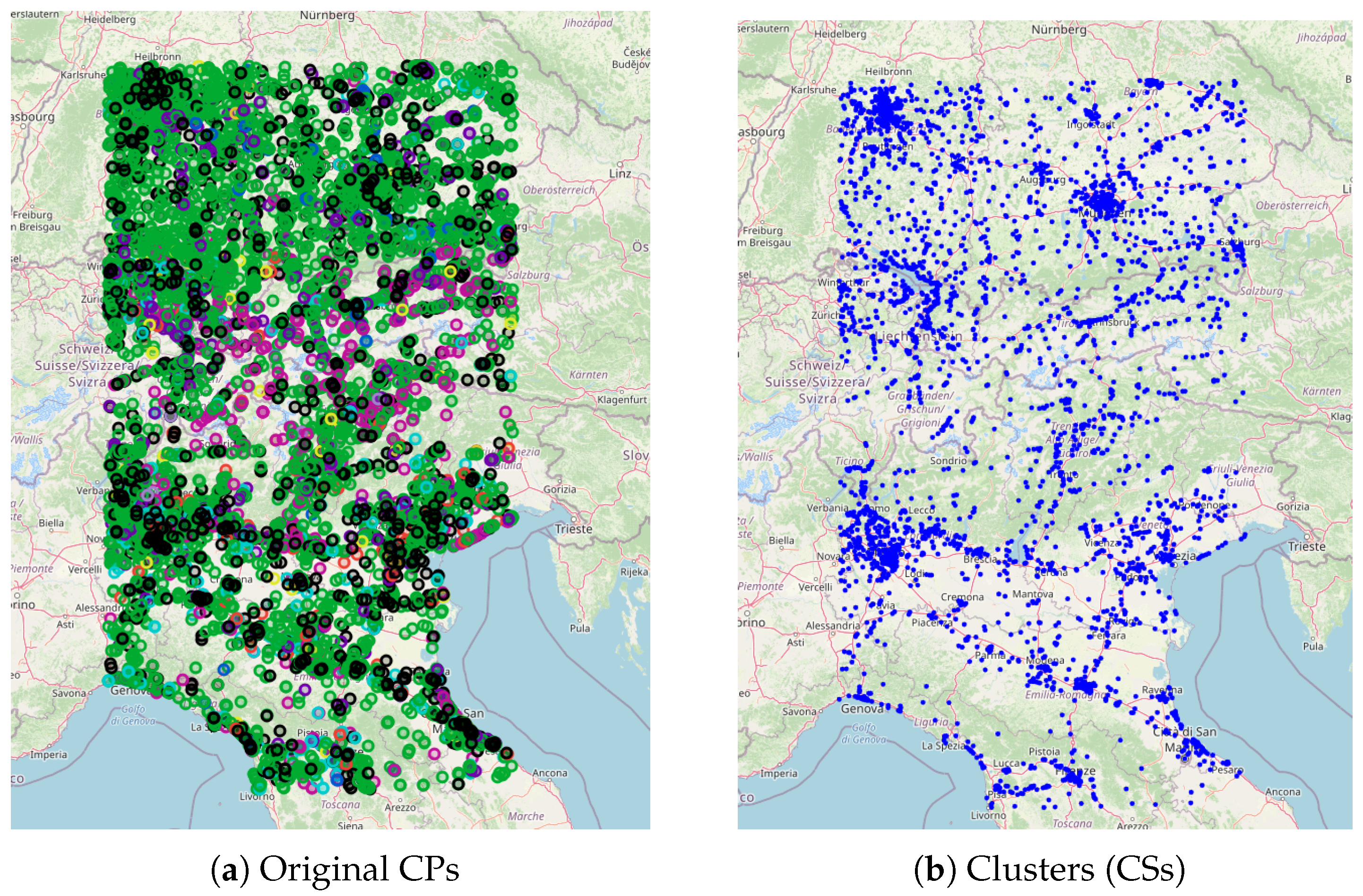
In this pre-processing step we generate a graph G = S O , D , A based on CP data and POI locations, which were provided by the project partners. To generate this graph, we create a set of CSs by clustering CPs, compute the modified weight of the arcs s ˜ i j , including the importance value of the CSs, and filter arcs by computing the resilience value for each arc in the graph. We describe each of these steps in the subsequent sections.

4.1.1. Clustering

We consider public charging interoperable CSs. Each such CS may group several CPs. At the same time, each CP may have different plug types. The data are typically provided in terms of CPs and not CSs. We generate CSs by clustering the CP data using the following procedure. We consider a maximum number n max of CPs per cluster, a minimum number n min of CPs per cluster, and the maximum geodesic distance d c between CPs in a cluster. These parameters are selected to provide the user with alternative CPs that are close enough to each other. The purpose of this procedure is to cover the case when a selected CP is not available at the moment of arrival, by providing alternatives to the user. Thus, the selection of the parameters depends on the characteristics of the geographical area, such as the total number of CPs and their sparsity.
Let C be the set of original CP locations, and  C ¯ be the set of clustered CPs, initially C ¯ = { } . The clustering algorithm starts by selecting a random CP i C , which initializes the first cluster. The coordinates of the center of the cluster are set to be the coordinates of CP i. Sequentially, we add CPs that are within a distance d c to the center of the cluster. Each time a CP is added, the coordinates of the center of the cluster are updated to be the average between the previous center and the coordinates of the new CP. A cluster is closed when either n max is reached or there are no other CPs available within d c . When a cluster is closed, a new random CP is selected, and the procedure is repeated with the remaining CPs in the dataset. The algorithm terminates when there are no other CPs available. If the final size of a cluster is lower than n min the cluster is removed from C ¯ . At the end of the procedure, each cluster is characterized by the coordinates of its center, and the information of each of the CPs in the cluster. In what follows we refer to a cluster of CPs as a CS and all distances are computed based on the center of the clusters.

4.1.2. Modified Arc Weights

In order to compute the modified weights of the arcs s ˜ i j as defined in Equation (1), we first compute the importance value σ j p associated with CS j and POI category p. To do so, we divide the POIs into three categories: (1) food (the user prefers to stop in clusters with restaurants), (2) nature (the user prefers to stop in clusters close to nature sites), and (3) shop (the user prefers to stop in places with several shops like malls, department stores, etc.). For each such category p, the importance value σ j p is computed as the number of available POIs within a distance d POI from the CS j S in the given category p P .

4.1.3. Resilience Value

For each arc ( i , j ) A we define a resilience value r i j to represent the availability of CSs within a critical distance from the actual road path represented by the arc. The resilience value ensures a minimum number of CSs are within a critical distance d r from the path in case of charging emergencies. To compute the resilience value, we divide the path between nodes i and j into sections of length d t . For each section k, we define the number of CSs that are within a distance of d r as C k = | { j S | d ( j , k ) d r } | , where d ( ) represents the shortest geodesic distance between CS j and section k. The resilience value r i j for the path between nodes i and j is defined as:
r i j = m e d ( { C k , k ( i , j ) A } ) ,
where m e d ( ) is the median value of the set. In our methodology, we consider a modified set of arcs A ¯ = { ( i , j ) A | r i j > r min , d i j > d r } , where r min is the minimum resilience value allowed for each arc. The later condition (i.e., d i j > d r ) implies that if two CSs are close enough to each other, the arc connecting them is considered to be resilient.

4.1.4. User Input Parameters

A user request is an origin–destination pair of locations. The user must also specify the EV type from a preset list. This choice establishes EV related parameters (i.e., the capacity Q of the battery, the average consumption of η , and the breaks in the charging curve B i ). Such parameters are obtained from the OpenEV repository [23]. In addition, the user may specify the starting SoC ( q start ), desired SoC at destination ( q end ), start time at the origin, and a rating for each POI category. These ratings are established with a slidebar that defines a weight parameter ranging from 0 to 100%. These user-defined weights are included in the model by directly multiplying them with the corresponding importance value σ j p . The user may also specify two types of time windows, one for lunch and one for night stays. Lunch stops are clusters that have at least one restaurant, whereas night stops consider hotels with CSs on their premises. Each optional intermediate stop is defined by a minimum start time γ w L , a maximum start time γ w U , and a minimum time that the EV needs to stop t w min . Finally, the user may select the plug types (“Type 2” and “Ccs”). CPs in CSs that do not match the selected plug types are discarded. Subsequently, the compatible CP with the maximum charging power in each CS is considered, ties are broken arbitrarily. Thus, the final address and CP specifications in the solution corresponds to the fastest compatible CP in the cluster.

4.1.5. Graph Reduction

In order to reduce computational run-times, we apply another filtering strategy using non EV-paths. In this step, we compute up to three alternative shortest paths between the origin and destination without considering CSs. These three paths are computed using mapbox [37]. We filter the graph G by only considering the CSs in S that are within a threshold of d f kilometers around the three non EV-paths. This step defines a new reduced graph G ˜ = S ˜ O , D , A ˜ , where S ˜ O , D is the filtered set of nodes and A ˜ A ¯ is the set of considered arcs between S ˜ O , D . In Figure 2, we illustrate the graph in this reduction step. The three solid lines show the three non EV-paths between the origin and destination. The colored areas show an approximation of the threshold from each path using d f = 50 km. All arcs and nodes that do not fall into the colored area are discarded.

4.2. Two-Step Algorithm

We solve the EVSPPWP on the modified graph G ˜ using a two-step algorithm. In the first step, we use a modified A * algorithm to establish the nodes where the user-defined time windows are going to be performed. The result of this step is a set of consecutive nodes, each one representing the location at which each time window is performed. Let N W S ˜ O , D be the ordered set of nodes selected by the algorithm to perform time windows in W . The output of the algorithm defines then | N W | + 1 legs. In what follows, we refer to legs as the paths to be performed from O to the first node in N W , the path between the ordered nodes in N W , and the path between the last node in N W and D . In the second step, we solve the FRVCP for each leg defined in the first step using the labeling algorithm proposed by Kullman et al. [6]. The final solution of the algorithm is the merged solution of each FRVCP instance defined by the legs in the first step.

4.2.1. A * Algorithm

We implement a modified A * search algorithm to find the nodes in which the user-specified time windows are performed in order to minimize the total travel time. For this search, we assume that recharging stops are only performed when the remaining energy in the battery is less than the energy needed to reach the next node. At each recharging stop, we assume that the EV is fully charged. The algorithm starts at node O and sequentially generates the tree of all paths to reach the next node using a best-first search until the destination node is reached. The best-first search is conducted by selecting the next node that minimizes the following objective:
f ( i ) = g ( i ) + h ( i )
where i is the current node, g ( i ) is the duration of the path from O to i, and  h ( i ) is an estimate of the duration of the shortest path from i to D . Duration computed in g ( i ) and h ( i ) include both travel and charging times. We use the modified travel times s ˜ i j as defined in Equation (1). By the use of a labeling search, the modified A * algorithm finds the nodes in G ˜ where times windows k W are performed, which define the legs in the following step.

4.2.2. FRVCP

We solve the FRVCP for each leg (i.e., considering the two extreme nodes of the legs as the fixed nodes) to determine the decisions on where and how much to charge at each recharging stop while minimizing the total travel time. To ensure the final SoC requirement q end is fulfilled at the destination, we add a dummy node at the end of each leg with a sufficient distance from the leg destination node, which is removed at the end of this step. We solve the problem for each leg exactly by the labeling algorithm of Kullman et al. [6] using the Python library frvcpy. The labeling algorithm returns the optimal energy-feasible path for each leg, i.e., the location of the stops, the amount to be charged at each stop, and the total duration. After computing the optimal solution for each leg, we merge together all solutions to obtain a single complete EV-path from O to D . The heuristic solution of the merged legs is the solution of the EVSPPWP.

5. Case Study

Within the eCharge4Drivers project and with the support of project partner Route 220 S.p.A. (Evway), we implemented our path planning methodology in the webpage available at https://planner.evway.net/, accessed on 15 May 2023. Specifically, the tool was implemented in five regions: Northern Italy and Regions North of Italy (NIRNI), Puglia, Greece, Turkey, and Spain. In Figure 3 we show the original CPs used in each of the five regions. For each region, the algorithm was tested using several combinations of origins and destinations. We implemented all parts of the algorithm in Python 3.8. In our tests, all run times for a single path were observed to be under 30 s. In the following, we focus on examples in the NIRNI area. In Section 5.1, we demonstrate how the graph is generated. In Section 5.2, we provide examples on various user inputs, and in Section 5.3, we demonstrate the results of our path planner on various origin–destination examples.

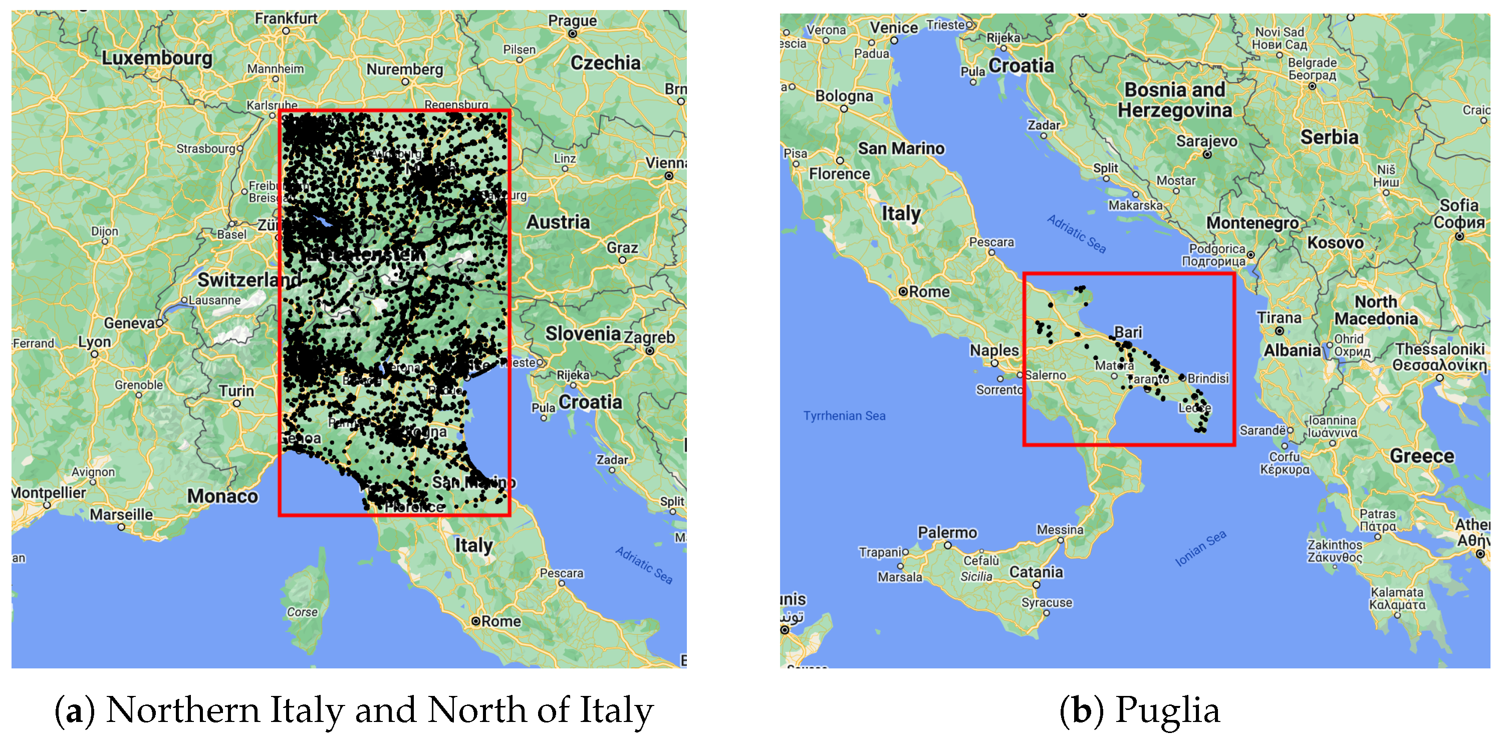
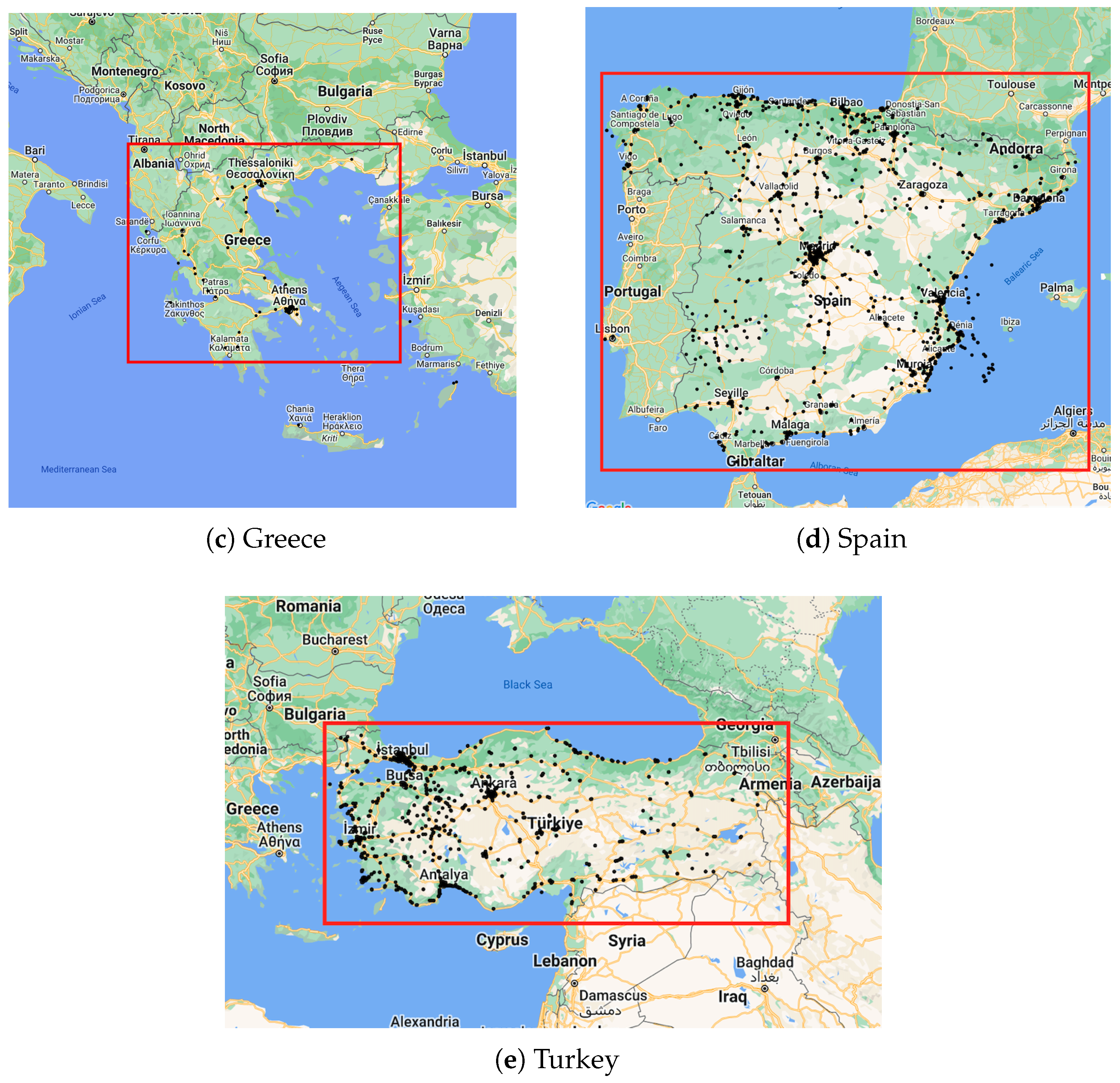
5.1. Graph Generation

The original dataset provided by the project partners contains 14,767 CPs, providing the location, address, and plug types. A second dataset contains the information on the POIs. This dataset was obtained by both the partner company and OpenStreetMap. Given the high density of CPs in the NIRNI area, we calibrated the three parameters of our clustering algorithm to have a balance between the number of clusters and the availability of CPs outside urban areas. We selected the following parameters in the graph generation step: n max = 15 , n min = 3 , d c = d POI = d t = l min = 1 km, d r = 10 km, d max = 300 km, d f = 50 km, μ = 0.5 , r min = 0.1 , and q min = 0.2 Q .
In Figure 4, we show the original CP locations and the final CPs clustered in CSs using the procedure described in Section 4.1.1. The resulting graph contains a total number of 3223 CSs.

5.2. User Input

The web interface provides users with the ability to select several inputs directly. These inputs include the start point, destination, and any intermediate waypoints for the trip. In addition, the user can choose the type of EV they will be using, selecting from available options in the OpenEV repository. This choice sets the parameters on battery capacity, average consumption, and charging curve breaks. The user can also set the battery SoC at the start of the trip, and desired SoC at the end of the trip. Additionally, the user can specify preferences for the three categories of stops, using sliders to set the level of importance for each category. The weights are directly multiplied by the importance value for each category. The interface also includes options for setting up lunch and hotel stops during the trip, and specifying their time windows. Finally, the user can choose the plug type they require, with options for “Type 2” and/or “Ccs” plugs.
As previously mentioned, we assume that the EV has an average consumption of η (kWh/km), which is multiplied by d i j to yield e i j . While there may be tools that allow a more accurate calculation of energy between nodes (e.g., accounting for vehicles dynamics according to geophysical properties of the traversed segments), such tools were not available to us. Specifically, we were able to query the systems of our project partners and obtain aggregate path information on a path between two addresses (e.g., distance, travel time). Therefore, as in most of the EVRP literature (see Kucukoglu et al. [3] for a classification of studies by their assumptions on energy consumption), we opted to estimate the energy consumption as a linear factor of the distance. We recognize that this is a shortcoming; yet, we note that, from an algorithmic perspective, energy consumption between nodes is an input. Therefore, the methodology will not change by more accurate energy consumption estimates.
The use of vehicle dynamics to obtain more accurate energy estimates entails the use of a more elaborate set of parameters related to each vehicle. To account for the geographical properties of the roads, one would need to retrieve detailed intersection by intersection road information between every pair of nodes. For example, in the NIRNI area, this corresponds to retrieving detailed intersection by intersection information for approximately 10,380,000 paths corresponding to the pairs of CSs. While such an additional step is computationally intensive, it would belong to the preprocessing stage since energy consumption is an input to our algorithm. From a computational perspective, we expect the run times not to be affected by changing the algorithm’s input.
After setting the user preferences on the web interface, the algorithm computes up to three path options between the origin and the destination. These three paths are based on the non EV paths as described in Section 4.1.5. Then the algorithm described in Section 4.2 is executed on each of the three paths establishing where to stop and how much to charge. In Figure 5a we show the three path options given by the algorithm for a trip between Milan, Italy, and Stuttgart, Germany. The figure consists of a left panel displaying the main results for each path, and a right panel displaying a map with the paths in different colors. Using the left panel, the user can select one of the paths for further details. After selecting the first path, as shown in Figure 5a, details on the place and duration of the recharging stops are shown in the left panel, while in the right panel, the selected path is displayed along with grey points representing alternative CPs. In Figure 5b, we compare the original path with a path using the option of adding a waypoint. Figure 6a shows the recommended path, whereas Figure 6b shows the path after the user selects a waypoint in Munich, Germany. The actual path and the charging stops are shown in green, and alternative CPs are shown in grey. The user may change a proposed CP by selecting an alternative CP. If an alternative CP is selected, the algorithm is re-run while fixing the selected CP.

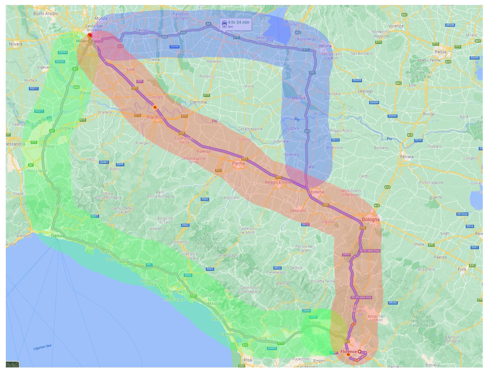
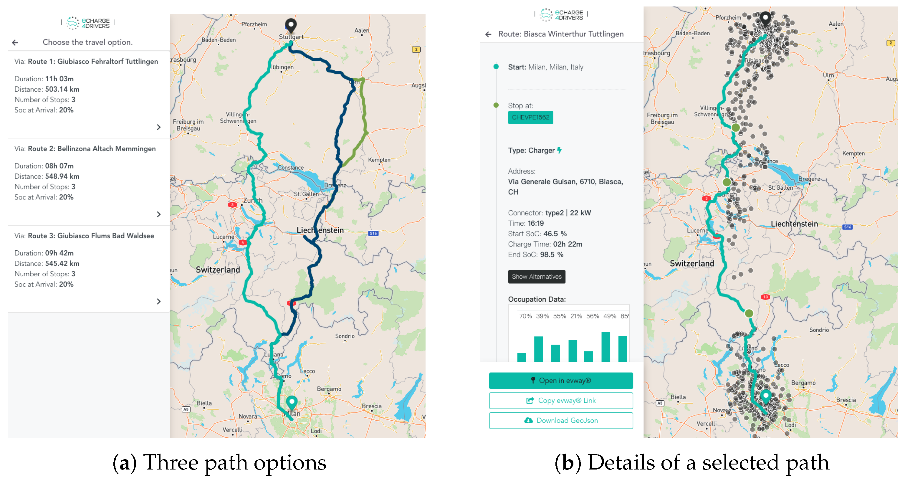
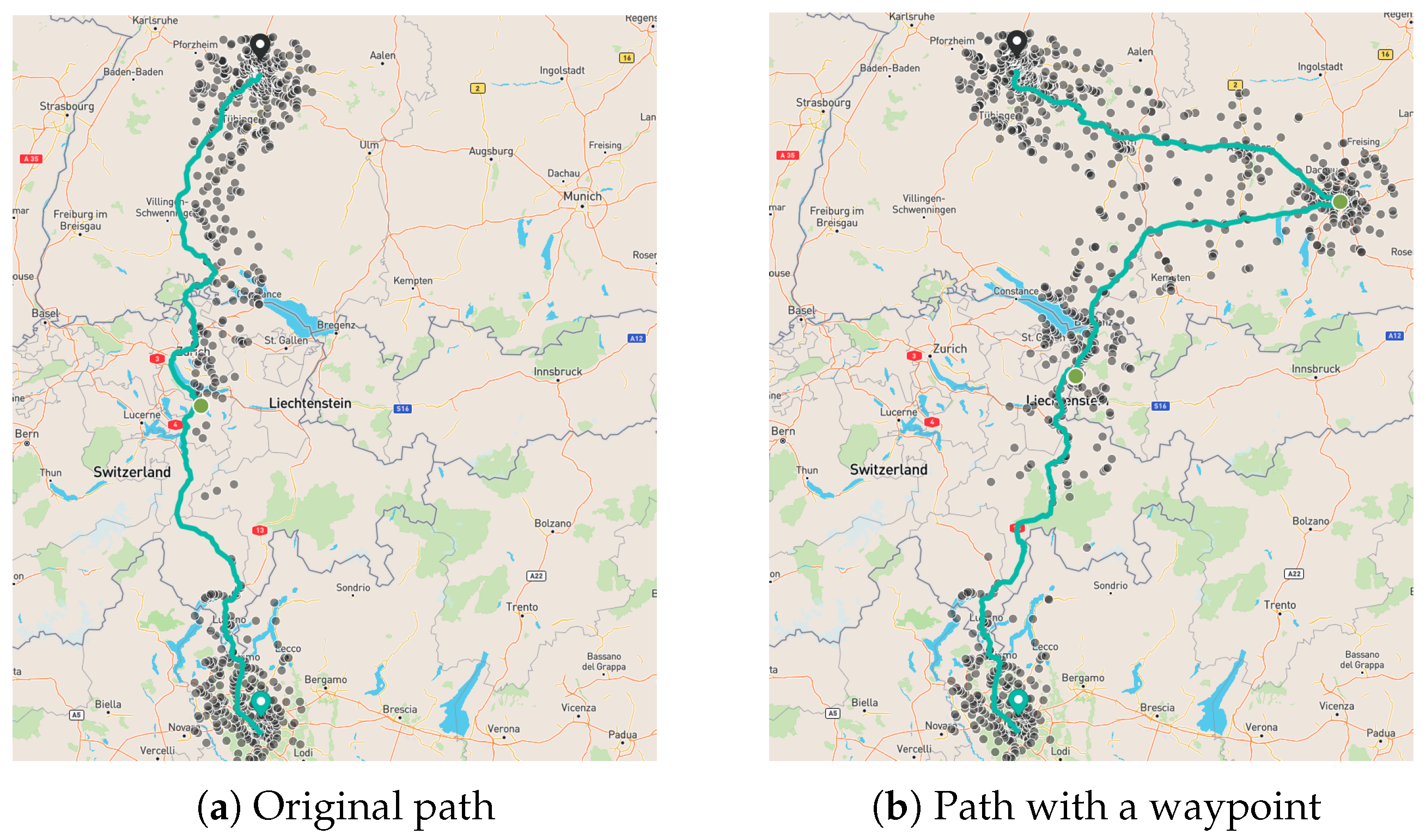
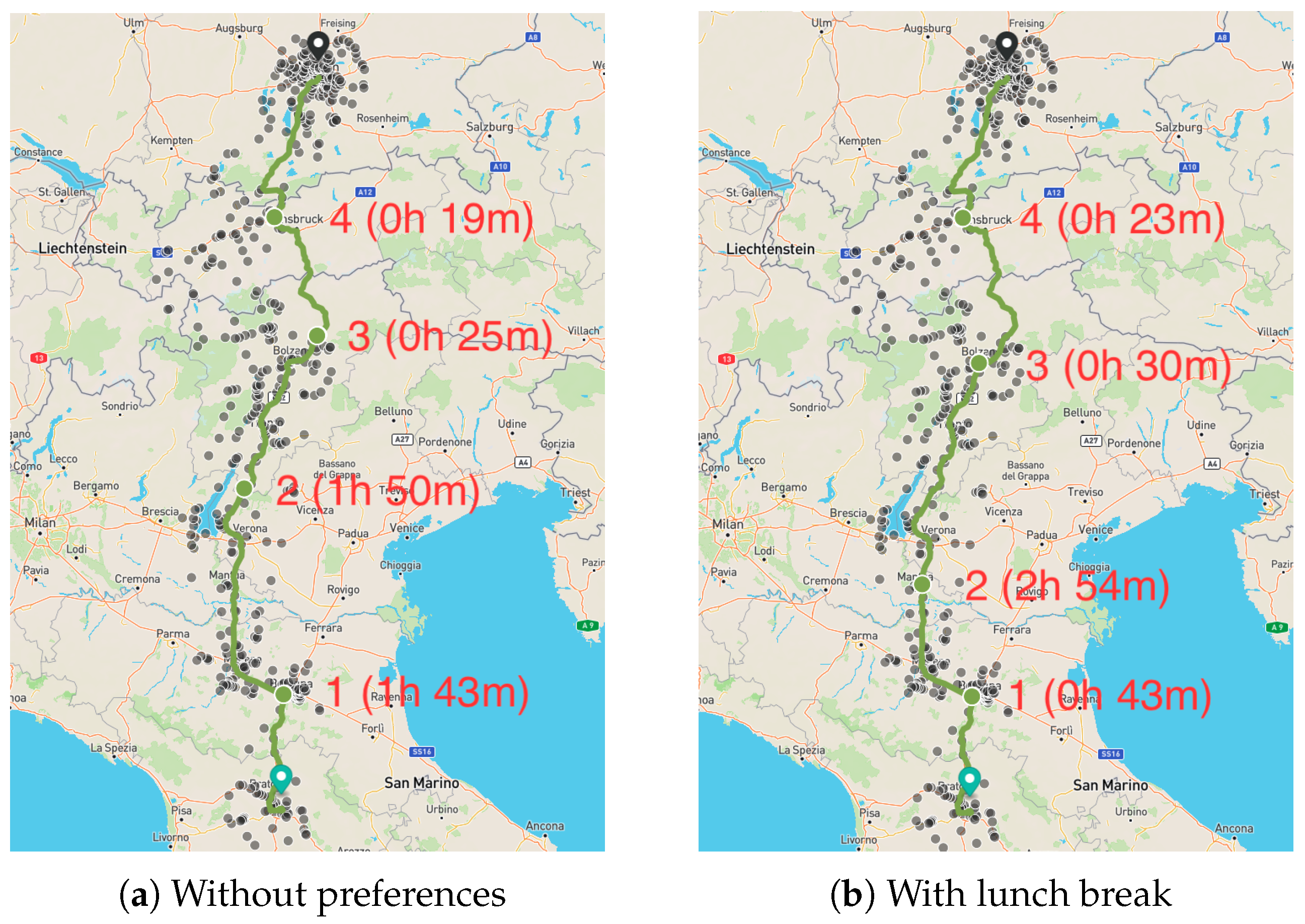
5.3. Origin–Destination Examples

We illustrate the use of our path planner methodology using three origin–destination pairs accounting for short, medium, and long-distance trips in the NIRNI area. For each trip, we compute the path using four configurations of user preferences: a base case without preferences, one assigning 100% to the shopping POI weight, one having a lunch stop, and one having a night stop. From the three possible path recommendations, we selected the fastest path. In all cases, we set the EV type to be BWM i3S 120Ah, a start SoC of 80%, and a desired end SoC of 20%. For the lunch break, the earliest arrival is set to 12:30, latest arrival is set to 13:30, and a duration of two hours is selected. For the night rest, the earliest desired check-in is 20:00, the latest check-in is 22:00, and the check-out is at 8:30. Table 1 reports the results for the three origin and destinations: Venice–Milan, Trento–Stuttgart, and Florence–Munich. All paths are set to start at 10:00, except from Venice–Milan and Trento–Stuttgart with night stops, which are set to start at 20:00 for its duration to match a night stop. For each path, we report the start time, end time, duration, distance, and number of recharging stops. We observe that the duration and distance of the trips vary depending on the preference selection. These differences are due to different selected stops and/or different charging times at the stops given the preferences. For example, trips with the night stop option have a notable increase in the total duration since this preference has a fixed check out at 8:30.
In Table 2, we show the address, start time, duration, SoC at start, and SoC at end for all four recharging stops in the path between Florence and Munich, for the four user preferences combinations. Except for the first stop, the addresses for the charging stops differ depending on the preference. A similar behavior can be observed in terms of the start time and duration of the charging stops. In Figure 7, we show a comparison of the paths without preferences and with lunch break. We can observe in the map that the first and last charging stops (1 and 4) are the same; however, they have different charging times. The intermediate charging stops (2 and 3) both show different locations and charging times.
In Table 3, we compare the duration, distance (km), and number of stops in a trip from Florence and Munich for four EV models. We show results using different starting SoCs, ranging from 60% to 100%, and the same desired SoC at arrival of 10%. We observe clear differences in the duration and number of stops in the trip depending on the selected EV type. Considering a starting SoC of 100%, the Tesla Roadster 2022 shows the fastest path with a duration of seven hours and five minutes with no recharging stops, while the slowest trip with Kia EV6 2WD 2021 lasts twelve hours and twenty-one minutes with two recharging stops. The same pattern can be seen when comparing EV models with lower starting SoC. As expected, we observe for all EV models a decrease in the number of stops from the starting SoC. In all cases, decreasing this value from 100% to 60% of SoC results in one additional recharging stop.

6. Conclusions

Given an origin and a destination, we proposed a path-planning methodology for EVs, considering user preferences. The main innovations in our methodology are the use of weights for three categories of POIs to reflect user preferences in the selection of CSs, the use of clustered CSs to ensure alternatives in the vicinity of CSs, the use of resilient paths, and allowing the user to define time windows for activities such as lunch and hotel stays. We divided our methodology into two parts. We first performed a pre-processing step in which we generate a graph with clustered CSs and resilient paths from raw CP and POI data. Then, we proposed a two-step algorithm to solve the shortest path problem. The final solution of our methodology is a heuristic solution for the EVSPPWP.
We conducted experiments for three origin–destination pairs in the NIRNI area, and for each trip, the fastest path is selected from four configurations of user preferences. We compared the duration, distance, and number of charging stops to demonstrate the usage of our methodology. In addition, we compared four EV models for a trip from Florence to Munich, which showed clear differences in duration and the number of stops, with the Tesla Roadster 2022 having the fastest path at seven hours and five minutes with no recharging stops when starting at 100% SoC, while a Kia EV6 2WD 2021 lasts twelve hours and twenty-one minutes with two recharging stops. Decreasing the starting SoC from 100% to 60% resulted in one additional recharging stop for all EV models.
An interesting extension to our methodology is to include the geophysical properties of the roads to obtain more accurate estimations of the energy consumption between CSs. Also, future extensions include considering dynamic planning, which accounts for dynamic energy consumption based on vehicle dynamics, driving conditions, traffic, road conditions, and other real-time restrictions.

Author Contributions

Conceptualization, M.C., M.D., O.J., F.M. and E.T.; methodology, M.C., M.D., O.J., F.M. and E.T.; software, M.C. and E.T.; validation, M.C., M.D., O.J., F.M. and E.T.; formal analysis, M.C., M.D., O.J., F.M. and E.T.; writing—original draft preparation, M.C. and O.J.; writing—review and editing, M.C. and O.J. All authors have read and agreed to the published version of the manuscript.

Funding

This work is a part of the eCharge4Drivers project. This project has received funding from the European Union Horizon 2020 research and innovation programme under grant agreement No. 875131. This content reflects only the author’s view and the European Commission is not responsible for any use that may be made of the information this publication contains.

Data Availability Statement

Not applicable.

Conflicts of Interest

The authors declare no conflict of interest.

Nomenclature

The following nomenclature is used in this manuscript:
EVElectric Vehicle
CPCharging Point
CSCharging Station
POIPoint of Interest
SoCState of Charge
kWhKilowatt-hour
EVSPPElectric Vehicle Shortest Path Problem
EVSPPWPElectric Vehicle Shortest Path Problem with time windows and user preferences
MILPMixed Integer Linear Programming
EVRPElectric Vehicle Routing Problem
FRVCPFixed Route Vehicle Charging Problem
TTDPTourist Trip Design Problem
EVRTPElectric Vehicle Routing Tour Planning
NIRNINorthern Italy and Regions North of Italy
S Set of charging stations
O Origin node
D Destination node
S O , D Set of nodes containing the origin O , destination D , and the set S
t start Start time at O
q start Initial SoC
q end Final SoC
q min Minimal energy at arrival
Δ Time spent charging at a CS
Φ i ( Δ ) 
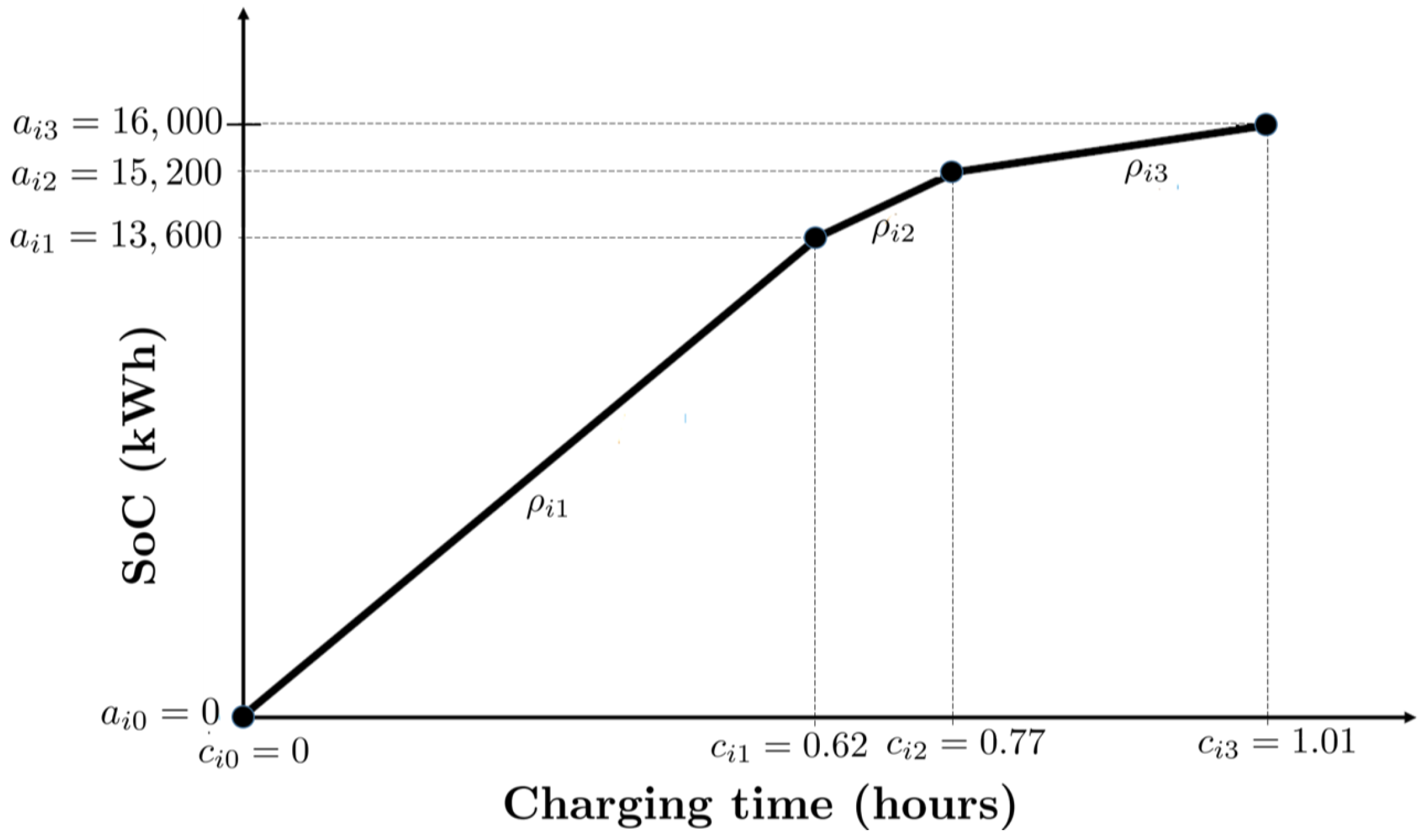
Piece-wise linear concave charging function of charging station i
G Graph
A Set of arcs in the graph G
t i j Driving time between nodes i and j
d i j Distance between nodes i and j
e i j Energy consumption between nodes i and j
η EV average consumption
QBattery capacity
B i Ordered set of breakpoints of the charging curve of CS i
c i k Charging time of breakpoint k B i
a i k SoC of breakpoint k B i
ρ i k Slope of the linear function that connects breakpoints ( c i , k 1 , a i , k 1 ) and ( c i k , a i k )
σ j p Importance value of j S for POI category p P
d max Maximum distance between arcs
μ Weight on the total importance value of the POIs with respect to travel time
P Set of POI categories
Δ j Time spent charging at CS j
W Set of ordered time windows that require a specific POI category
γ w L Minimum start time of time window w
γ w U Maximum start time of time window w
t w min Minimum time that the EV needs to stop for time window w
S w Set of CSs with POIs in their neighborhood that match the POI specified for w W
s ˜ i j Modified weight of the arc between nodes i and j
q ̲ i SoC when the EV arrives at i
q ¯ i SoC when the EV departs from i
h ̲ i Start time for charging an EV at i
h ¯ i End time for charging an EV at i
λ ̲ i k Coefficients associated with the breakpoint ( c i k , a i k ) when the EV enters i
λ ¯ i k Coefficients associated with the breakpoint ( c i k , a i k ) when the EV leaves i
w ̲ i k Binary variable equal to 1 when the SoC is in [ a i , k 1 , a i k ] , when the EV enters i
w ¯ i k Binary variable equal to 1 when the SoC is in [ a i , k 1 , a i k ] , when the EV leaves i
τ ̲ i Time when the EV arrives at i
τ ¯ i Time when the EV departs from i
x i j Binary variable equal to 1 if the EV uses arc ( i , j )
y j w Binary variable equal to 1 if the EV stops in j in time window w
d POI Distance threshold for considering POIs around a CS
r i j Resilience value of the arc between nodes i and j
d r Critical distance for ensuring availability of CSs
d t Length of a section in which the resilience value is computed
C k Number of CSs within a distance of d r from section k
d f Threshold distance around the non EV-paths
G ˜ Reduced graph
S ˜ O , D Filtered set of nodes
A ˜ Set of considered arcs between S ˜ O , D
N W Ordered set of nodes selected by the algorithm to perform time windows in W

References

  1. EEA. Average Carbon Dioxide Emissions from New Cars Registered in EUROPE Decreased by 12% in 2020. 2022. Available online: https://www.eea.europa.eu/highlights/average-carbon-dioxide-emissions-from (accessed on 13 April 2023).
  2. Martins, L.d.C.; Tordecilla, R.D.; Castaneda, J.; Juan, A.A.; Faulin, J. Electric vehicle routing, arc routing, and team orienteering problems in sustainable transportation. Energies 2021, 14, 5131. [Google Scholar] [CrossRef]
  3. Kucukoglu, I.; Dewil, R.; Cattrysse, D. The electric vehicle routing problem and its variations: A literature review. Comput. Ind. Eng. 2021, 161, 107650. [Google Scholar] [CrossRef]
  4. Froger, A.; Jabali, O.; Mendoza, J.E.; Laporte, G. The electric vehicle routing problem with capacitated charging stations. Transp. Sci. 2022, 56, 460–482. [Google Scholar] [CrossRef]
  5. Sánchez, D.G.; Tabares, A.; Faria, L.T.; Rivera, J.C.; Franco, J.F. A Clustering Approach for the Optimal Siting of Recharging Stations in the Electric Vehicle Routing Problem with Time Windows. Energies 2022, 15, 2372. [Google Scholar] [CrossRef]
  6. Kullman, N.D.; Froger, A.; Mendoza, J.E.; Goodson, J.C. frvcpy: An open-source solver for the fixed route vehicle charging problem. INFORMS J. Comput. 2021, 33, 1277–1283. [Google Scholar] [CrossRef]
  7. A Better Route Planner. 2023. Available online: https://abetterrouteplanner.com (accessed on 15 March 2023).
  8. ZapMapEV. 2023. Available online: https://www.zap-map.com (accessed on 15 March 2023).
  9. PlugShare. 2023. Available online: https://www.plugshare.com (accessed on 15 March 2023).
  10. Schiffer, M.; Schneider, M.; Walther, G.; Laporte, G. Vehicle routing and location routing with intermediate stops: A review. Transp. Sci. 2019, 53, 319–343. [Google Scholar] [CrossRef]
  11. Erdoğan, S.; Miller-Hooks, E. A green vehicle routing problem. Transp. Res. Part E Logist. Transp. Rev. 2012, 48, 100–114. [Google Scholar] [CrossRef]
  12. Schneider, M.; Stenger, A.; Goeke, D. The electric vehicle-routing problem with time windows and recharging stations. Transp. Sci. 2014, 48, 500–520. [Google Scholar] [CrossRef]
  13. Felipe, Á.; Ortuño, M.T.; Righini, G.; Tirado, G. A heuristic approach for the green vehicle routing problem with multiple technologies and partial recharges. Transp. Res. Part E Logist. Transp. Rev. 2014, 71, 111–128. [Google Scholar] [CrossRef]
  14. Hiermann, G.; Hartl, R.F.; Puchinger, J.; Vidal, T. Routing a mix of conventional, plug-in hybrid, and electric vehicles. Eur. J. Oper. Res. 2019, 272, 235–248. [Google Scholar] [CrossRef]
  15. Goeke, D.; Schneider, M. Routing a mixed fleet of electric and conventional vehicles. Eur. J. Oper. Res. 2015, 245, 81–99. [Google Scholar] [CrossRef]
  16. Keskin, M.; Çatay, B. Partial recharge strategies for the electric vehicle routing problem with time windows. Transp. Res. Part C Emerg. Technol. 2016, 65, 111–127. [Google Scholar] [CrossRef]
  17. Montoya, A.; Guéret, C.; Mendoza, J.E.; Villegas, J.G. The electric vehicle routing problem with nonlinear charging function. Transp. Res. Part B Methodol. 2017, 103, 87–110. [Google Scholar] [CrossRef]
  18. Pelletier, S.; Jabali, O.; Laporte, G. The electric vehicle routing problem with energy consumption uncertainty. Transp. Res. Part B Methodol. 2019, 126, 225–255. [Google Scholar] [CrossRef]
  19. Montoya, A.; Guéret, C.; Mendoza, J.E.; Villegas, J.G. A multi-space sampling heuristic for the green vehicle routing problem. Transp. Res. Part C Emerg. Technol. 2016, 70, 113–128. [Google Scholar] [CrossRef]
  20. Andelmin, J.; Bartolini, E. An exact algorithm for the green vehicle routing problem. Transp. Sci. 2017, 51, 1288–1303. [Google Scholar] [CrossRef]
  21. Froger, A.; Mendoza, J.E.; Jabali, O.; Laporte, G. Improved formulations and algorithmic components for the electric vehicle routing problem with nonlinear charging functions. Comput. Oper. Res. 2019, 104, 256–294. [Google Scholar] [CrossRef]
  22. Desaulniers, G.; Errico, F.; Irnich, S.; Schneider, M. Exact algorithms for electric vehicle-routing problems with time windows. Oper. Res. 2016, 64, 1388–1405. [Google Scholar] [CrossRef]
  23. OpenEV. GitHub-Chargeprice/Open-ev-Data. 2022. Available online: https://github.com/chargeprice/open-ev-data (accessed on 15 March 2023).
  24. Zündorf, T. Electric Vehicle Routing with Realistic Recharging Models. Master’s Thesis, Karlsruhe Institute of Technology, Karlsruhe, Germany, 2014, unpublished. [Google Scholar]
  25. Sweda, T.M.; Dolinskaya, I.S.; Klabjan, D. Adaptive routing and recharging policies for electric vehicles. Transp. Sci. 2017, 51, 1326–1348. [Google Scholar] [CrossRef]
  26. Baum, M.; Dibbelt, J.; Gemsa, A.; Wagner, D.; Zündorf, T. Shortest feasible paths with charging stops for battery electric vehicles. Transp. Sci. 2019, 53, 1627–1655. [Google Scholar] [CrossRef]
  27. Baum, M.; Dibbelt, J.; Pajor, T.; Sauer, J.; Wagner, D.; Zündorf, T. Energy-optimal routes for battery electric vehicles. Algorithmica 2020, 82, 1490–1546. [Google Scholar] [CrossRef]
  28. Aljohani, T.M.; Mohammed, O. A Real-Time Energy Consumption Minimization Framework for Electric Vehicles Routing Optimization Based on SARSA Reinforcement Learning. Vehicles 2022, 4, 1176–1194. [Google Scholar] [CrossRef]
  29. Aljohani, T.M.; Ebrahim, A.; Mohammed, O. Real-Time metadata-driven routing optimization for electric vehicle energy consumption minimization using deep reinforcement learning and Markov chain model. Electr. Power Syst. Res. 2021, 192, 106962. [Google Scholar] [CrossRef]
  30. Roberti, R.; Wen, M. The electric traveling salesman problem with time windows. Transp. Res. Part E Logist. Transp. Rev. 2016, 89, 32–52. [Google Scholar] [CrossRef]
  31. Ruiz-Meza, J.; Montoya-Torres, J.R. A systematic literature review for the tourist trip design problem: Extensions, solution techniques and future research lines. Oper. Res. Perspect. 2022, 9, 100228. [Google Scholar] [CrossRef]
  32. Gavalas, D.; Konstantopoulos, C.; Mastakas, K.; Pantziou, G. A survey on algorithmic approaches for solving tourist trip design problems. J. Heuristics 2014, 20, 291–328. [Google Scholar] [CrossRef]
  33. Wang, Y.W.; Lin, C.C.; Lee, T.J. Electric vehicle tour planning. Transp. Res. Part D Transp. Environ. 2018, 63, 121–136. [Google Scholar] [CrossRef]
  34. Karbowska-Chilinska, J.; Chociej, K. Genetic algorithm for generation multistage tourist route of electrical vehicle. In Proceedings of the International Conference on Computer Information Systems and Industrial Management, Bialystok, Poland, 16–18 October 2020; Springer: Berlin, Germany, 2020; pp. 366–376. [Google Scholar]
  35. Cortés-Murcia, D.L.; Afsar, H.M.; Prodhon, C. Multi-period profitable tour problem with electric vehicles and mandatory stops. Int. J. Sustain. Transp. 2022, 17, 473–489. [Google Scholar] [CrossRef]
  36. Cassia, A.; Jabali, O.; Malucelli, F.; Pascoal, M. The electric vehicle shortest path problem with time windows and prize collection. In Proceedings of the 2022 17th Conference on Computer Science and Intelligence Systems (FedCSIS), Sofia, Bulgaria, 4–7 September 2022; IEEE: Piscataway, NJ, USA, 2022; pp. 313–322. [Google Scholar]
  37. Mapbox. Mapbox Optimization Tool. 2023. Available online: https://www.mapbox.com (accessed on 15 March 2023).
Figure 1. Example of a piece-wise linear approximation for a CS i S with a power of 22 kWh adapted from Montoya et al. [17].
Energies 16 04173 g001
Figure 2. Illustration of the graph reduction phase for three non EV-paths from Florence to Milan, using a threshold of d f = 50 km.
Energies 16 04173 g002
Figure 3. The five regions in which the path-planning methodology was tested.
Energies 16 04173 g003aEnergies 16 04173 g003b
Figure 4. (a) Original 14,767 CPs colored by plug type, and (b) resulting 3223 clusters of CPs in the NIRNI area.
Energies 16 04173 g004
Figure 5. Example of three path options for a trip from Milan to Stuttgart on the web interface.
Energies 16 04173 g005
Figure 6. Example of the addition of one waypoint in Munich, for a trip between Milan and Stuttgart.
Energies 16 04173 g006
Figure 7. Comparison of paths between Florence and Munich using (a) no user preferences and (b) selecting a lunch break of two hours, with charging stop number and duration.
Energies 16 04173 g007
Table 1. Path details for three origin–destination pairs. For each pair, four different user preferences are selected.
OriginDestinationPreferenceStart TimeEnd TimeDurationDistance (km)Charging Stops
VeniceMilan-10:0015:1705 h 17 min268.581
100% weight for shopping10:0013:3603 h 36 min269.871
Lunch10:0015:1605 h 16 min274.322
Night20:0010:3114 h 31 min268.581
TrentoStuttgart-10:0017:247 h 24 min499.843
100% weight for shopping10:0018:1508 h 15 min506.253
Lunch10:0018:1608 h 16 min500.403
Night20:0013:1017 h 10 min500.403
FlorenceMunich-10:0021:5411 h 54 min649.154
100% weight for shopping10:0022:5112 h 51 min651.754
Lunch10:0021:5611 h 56 min639.944
Night10:0010:0924 h 09 min649.154
Table 2. Recharging stop decisions details for a trip from Florence to Munich. Results are shown for four different user preferences.
PreferenceStopAddressStart TimeDurationSoC Start (%)SoC End (%)
-1Via Isonzo 16, 40033, IT11:1401 h 43 min36.4100.0
2Via Dante 14, 38063, IT14:4801 h 50 min23.176.5
3Schindergries Parking, 39043, IT18:0500 h 25 min20.075.0
4Roßhütte 419, 6100, AT19:5400 h 19 min27.871.5
100% weight for shopping1Via Isonzo 16, 40033, IT11:5901 h 36 min36.4100.0
2Via Dante 14, 38063, IT15:3301 h 50 min23.176.5
3Schindergries Parking, 39043, IT18:5001 h 02 min20.0100.0
4Marienpl. 17, 82467, DE21:4900 h 39 min39.058.0
Lunc h1Via Isonzo 16, 40033, IT11:1400 h 43 min36.463.4
2Via del Commercio 33, 46030, IT13:0302 h 54 min20.094.8
3Via Lancia - Lanciastraße 14, 39100, IT17:4200 h 30 min20.079.0
4Roßhütte 419, 6100, AT19:5300 h 23 min20.071.5
Night1Via Isonzo 16, 40033, IT11:1401 h 43 min36.4100.0
2Via Dante 14, 38063, IT14:4801 h 50 min23.176.5
3Schindergries Parking, 39043, IT18:0500 h 21 min20.067.2
4Roßhütte 419, 6100, AT19:5112 h 38 min20.0100.0
Table 3. Duration, distance (km), and number of stops for a trip between Florence and Munich for different EV models and SoCs at start.
EV ModelSoC at Start (%)
60708090100
Tesla Roadster 2022Duration09 h 45 min08 h 51 min07 h 53 min07 h 05 min07 h 05 min
Distance654.94652.11652.11648.42648.42
Stops11100
Tesla Model Y Long Range 2020Duration12 h 05 min11 h 20 min10 h 40 min10 h 06 min9 h 24 min
Distance659.21655.19655.19658.57652.04
Stops22221
BMW - i3S - 120 A h 2020Duration11 h 16 min12 h 10 min11 h 54 min12 h 10 min11 h 33 min
Distance643.4649.15649.15638.2639.6
Stops44433
Kia EV6 2WD 2021Duration12 h 12 min15 h 05 min14 h 33 min12 h 15 min12 h 21 min
Distance662.49662.63662.62663.13658.61
Stops32222
Disclaimer/Publisher’s Note: The statements, opinions and data contained in all publications are solely those of the individual author(s) and contributor(s) and not of MDPI and/or the editor(s). MDPI and/or the editor(s) disclaim responsibility for any injury to people or property resulting from any ideas, methods, instructions or products referred to in the content.

