Short-Term Load Forecasting Models: A Review of Challenges, Progress, and the Road Ahead

Abstract

Short-term load forecasting (STLF) is critical for the energy industry. Accurate predictions of future electricity demand are necessary to ensure power systems’ reliable and efficient operation. Various STLF models have been proposed in recent years, each with strengths and weaknesses. This paper comprehensively reviews some STLF models, including time series, artificial neural networks (ANNs), regression-based, and hybrid models. It first introduces the fundamental concepts and challenges of STLF, then discusses each model class’s main features and assumptions. The paper compares the models in terms of their accuracy, robustness, computational efficiency, scalability, and adaptability and identifies each approach’s advantages and limitations. Although this study suggests that ANNs and hybrid models may be the most promising ways to achieve accurate and reliable STLF, additional research is required to handle multiple input features, manage massive data sets, and adjust to shifting energy conditions.

1. Introduction

The efficient operation and planning of the power system require accurate load forecasting. Short-term load forecasting (STLF) is critical in power system applications, as it allows the optimal scheduling of energy resources and the efficient management of energy storage systems [1]. Short-term load forecasting (STLF) is a crucial task for the energy industry, as accurate predictions of future electricity demand are necessary to ensure power systems’ reliable and efficient operation [2]. STLF models, shown in Figure 1, involve predicting the electricity demand for the next few hours, days, or weeks, typically up to a maximum of one month. Accurate load forecasting is essential for efficient energy planning, scheduling, and dispatch, as it helps to balance supply and demand, minimize production costs, and avoid power outages [3]. Various STLF models have been proposed in recent years, each with strengths and weaknesses [4]. These models include time series, artificial neural networks (ANNs), regression-based, and hybrid models. Time series models use historical load data to identify patterns and trends in the load profile and make predictions based on statistical and mathematical techniques such as autoregressive integrated moving averages (ARIMA) and exponential smoothing [5]. ANNs are machine learning models that can capture complex nonlinear relationships between input and output variables and can be trained on large and diverse datasets using backpropagation algorithms [6]. Regression-based models use linear or nonlinear regression analysis to establish causal relationships between load and environmental factors such as temperature, humidity, and time of day [7]. Hybrid models combine the strengths of multiple model classes, such as ANNs and time series models, to achieve better accuracy and robustness [8]. Despite the growing interest in STLF, several challenges and limitations are associated with each model class. Time series models may be limited by their inability to capture long-term trends and non-stationary load data and their sensitivity to data outliers and missing values. ANNs may be limited by their computational complexity, interpretability, and overfitting, as well as their susceptibility to noise and bias in the training data [9]. Regression-based models may be limited by their assumptions of linearity and additivity in the input–output relationships and their difficulty in handling categorical or non-numeric data [10]. Hybrid models may be limited by their complexity, parameter tuning, and scalability, as well as their potential overfitting and data redundancy [11]. To address these challenges, it is essential to compare and evaluate the performance of different STLF models on real-world load data using a variety of metrics and validation techniques.

Given the fast-paced progress in machine learning, artificial intelligence, and data processing methods, there is a continuous need for updated reviews encompassing the latest developments in short-term load forecasting (STLF) models. This review paper aims to cover these recent advancements and provide insights into state-of-the-art models, which might not be covered in older reviews. As the world moves toward a more sustainable energy future, accurate load forecasting is becoming even more critical in managing power systems’ increasing complexity and variability.

Table 1. Contributions and limitations of recent publications.

Refs.	Contributions	Limitations
[12]	A comprehensive review of deep learning techniques Detailed analysis of CNNs, LSTMs, and GRUs	Limited to deep learning techniques Lacks comparison with traditional or hybrid methods
[13]	Comparative study of hybrid models Clear analysis of model performance	Limited to specific hybrid combinations Lacks analysis of individual model components
[14]	Meta-analysis of ensemble learning techniques Thorough discussion of bagging, boosting, and stacking	Limited to ensemble techniques Does not consider standalone models
[15]	Case study on feature selection in load forecasting Demonstrates the potential of feature selection	Limited to one case study Lacks generalization to other scenarios
[16]	Explores Bayesian neural networks for forecasting. Explanation of methodology and advantages	Limited to probabilistic methods Lacks comparison with deterministic approaches

lists the contributions and limitations of the latest published articles on the topic of short-term load forecasting.

This review paper highlights the challenges in the field of short-term load forecasting and suggests suitable solutions. The latest development in statistical, hybrid, and intelligent STLF models is explored with mathematical analysis. The various features of deep learning strategies are analyzed. This in-depth analysis is valuable for researchers and practitioners, enabling them to make informed decisions when selecting and applying appropriate forecasting models. Our paper presents a critical analysis of the models’ advantages and limitations, offering insights into potential improvements and suggesting new approaches that can enhance the performance of STLF models. This contribution aids in advancing the field by addressing existing challenges and identifying areas for future research.

2. Challenges and Solutions

One of the critical challenges in developing accurate STLF models is dealing with the dynamic nature of load data. Weather, economic conditions, and consumer behavior affect load data, which can change over time [17]. Therefore, STLF models need to be able to adapt to changes in the underlying data-generating process. One approach to dealing with non-stationary data is using time-varying models, such as autoregressive moving average (TVARMA) models [13]. TVARMA models allow autoregressive coefficients and moving average terms to vary over time, allowing the model to capture changes in the underlying data-generating process. TVARMA models have been shown to outperform stationary models such as ARIMA in some STLF applications. Another approach to dealing with non-stationary data is to use machine learning models, such as deep learning models [18]. Deep learning models, such as deep neural networks (DNNs), can automatically learn complex patterns and relationships and adapt to changes in the data-generating process [18]. However, training and implementing deep learning models require much data and computational resources.

In addition to dealing with non-stationary data, another challenge in STLF is uncertainty and risk management. STLF models provide point forecasts of the future load values but do not provide information on the uncertainty or risk associated with the forecasts. Therefore, there is a need for models that can provide probabilistic forecasts, such as quantile regression models [19]. Quantile regression models provide estimates of the conditional quantiles of the load distribution, allowing for the construction of prediction intervals and risk assessment. Quantile regression models are effective in providing probabilistic forecasts in STLF applications. One more strategy to deal with uncertainty and risk management is scenario-based forecasting. Scenario-based forecasting involves generating multiple scenarios of the future load values based on the different assumptions of the underlying data-generating process [20]. Scenario-based forecasting allows for assessing the risk associated with different scenarios and can inform decision-making under uncertainty.

STLF models must also be scalable and adaptable to different power systems and operating conditions. Power systems vary in size, complexity, and generation mix, and STLF models must be able to accommodate these variations [21]. Transfer learning is one approach to developing scalable and adaptable STLF models. Transfer learning involves using a pre-trained model on one power system and adapting it to another. Transfer learning can reduce the data and computational resources required to train a new model and enable the transfer of knowledge and expertise across different power systems. Using meta-learning is a different strategy for developing scalable and adaptable STLF models. Meta-learning involves learning the optimal model and hyperparameters for a new power system based on the characteristics of the power system and the available data. Meta-learning can reduce the time and resources required to develop a new STLF model and enable the development of models tailored to the power system’s specific characteristics [22].

Another challenge in STLF is dealing with the uncertainty and variability of renewable energy sources, such as wind and solar. Renewable energy sources are highly variable and uncertain, and their integration into power systems can affect the accuracy of STLF models [23]. One method of handling the variability of renewable energy sources is to use hybrid models that combine STLF and renewable energy forecasting models. Renewable energy forecasting models use weather data and other predictors to forecast the output of renewable energy sources, such as wind and solar. Hybrid models can combine the forecasts of the STLF models with the forecasts of the renewable energy forecasting models, improving the load forecasts’ accuracy [24]. Another strategy to cope with the variability of renewable energy sources is the use of demand response and energy storage. Demand response involves incentivizing consumers to reduce their electricity consumption during periods of high demand or low renewable energy output, while energy storage involves storing excess renewable energy for later use. Demand response and energy storage can reduce the variability and uncertainty of renewable energy sources and improve STLF model accuracy.

Another difficulty in STLF is addressing the high-dimensional and complex nature of the data. STLF models often require many predictors, such as weather data, holiday schedules, and economic indicators [25]. However, using too many predictors can lead to overfitting and reduced accuracy. One strategy for handling the high-dimensional and complex nature of the data is to use feature selection techniques. Feature selection techniques involve selecting a subset of the most relevant predictors for the forecasting task [26]. This strategy can reduce the number of predictors used in the model, reduce overfitting, and improve the accuracy of the forecasts. Another method for handling the high-dimensional and complex nature of the data is to use dimensionality reduction techniques. Dimensionality reduction techniques involve transforming the data into a lower-dimensional space while preserving the essential information. This technique can reduce the number of predictors used in the model, reduce the computational resources required, and improve the accuracy of the forecasts [27].

STLF also faces the difficulty of the non-Gaussian and heavy-tailed nature of the load data. Load data often exhibits non-Gaussian and heavy-tailed distributions, which can violate the assumptions of many STLF models [28]. One method to deal with the non-Gaussian and heavy-tailed nature of the load data is to use robust STLF models. Robust STLF models are designed to be less sensitive to outliers and heavy-tailed distributions and can provide more accurate forecasts in these scenarios. Another technique to deal with the non-Gaussian and heavy-tailed nature of the load data is to use distributional STLF models [29]. Distributional STLF models model the entire distribution of the load data rather than just the mean, allowing for the estimation of quantiles, prediction intervals, and risk assessment.

A further challenge in STLF is dealing with the nonlinear and non-monotonic relationships between the load data, weather data, and other predictors [30]. STLF models often require nonlinear and non-monotonic models to capture these relationships. One strategy to cope with nonlinear and non-monotonic relationships is to use non-parametric models, such as decision trees or random forests [31]. Non-parametric models can handle nonlinear and non-monotonic relationships and automatically learn complex patterns and relationships in the data. One more approach to dealing with nonlinear and non-monotonic relationships is to use kernel-based models, such as kernel regression or support vector machines [32]. Kernel-based models can handle nonlinear and non-monotonic relationships and be more computationally efficient than non-parametric models.

Another critical challenge in STLF is dealing with the spatial dimension of load data. Load data varies over time and space, and STLF models must account for spatial dependencies and heterogeneity. One way to deal with the spatial dimension of load data is to use spatial–temporal models. Spatial–temporal models account for the spatial and temporal dependencies of the load data and can provide more accurate forecasts by incorporating information from neighboring locations [33]. Another strategy to handle the spatial dimension of load data is to use clustering and spatial interpolation techniques. Clustering techniques involve grouping similar places based on their load patterns. By contrast, spatial interpolation techniques involve estimating the load values at unobserved locations based on the load values at nearby observed locations.

In addition to the challenges mentioned above, STLF models must be transparent and interpretable. STLF models are used in critical decision-making processes, such as load shedding and demand response, and power system operators and decision-makers need to understand their results quickly. One method of developing transparent and interpretable STLF models is to use explainable artificial intelligence (XAI) techniques [34]. XAI techniques involve developing models that explain their decisions and predictions. This can increase the transparency and trustworthiness of the models and enable power system operators and decision-makers to better understand the underlying factors that contribute to the load forecasts. Another way to develop transparent and interpretable STLF models is to use causal inference techniques [35]. Causal inference techniques involve developing models that can identify the causal relationships between the load data and other predictors and provide insights into the underlying drivers of load demand.

Finally, another challenge in STLF is dealing with the lack of data and data quality issues. STLF models require a large amount of data to train and validate, and the data quality can affect the forecasts’ accuracy [36]. Data augmentation techniques are one method to deal with the lack of data and data quality issues. Data augmentation techniques involve generating new data from the existing data by adding noise, perturbing the data, or generating synthetic data. Data augmentation can increase the data available for training and improve the model’s generalization. Another way to deal with the lack of data and data quality issues is to use transfer learning and domain adaptation techniques [37]. These techniques can reduce the data required to train a new model and enable the transfer of knowledge and expertise across different power systems.

3. Development in STLF Models

Traditional STLF models use historical load, weather, and calendar data as input features. However, the availability of new data sources, such as social media data and smart meter data, presents an opportunity to develop more accurate and robust STLF models. Advanced machine learning techniques, such as deep learning and reinforcement learning, have shown great potential in improving the accuracy of STLF models [38]. Deep learning techniques can automatically learn complex patterns and relationships in the data, while reinforcement learning can learn to optimize actions based on feedback from the environment [39]. Probabilistic forecasting provides a measure of uncertainty around the point forecast, which can help power system operators make more informed decisions in the face of uncertainty. Various STLF models have been developed, but they can be broadly classified into statistical, intelligent, and hybrid [40]. Figure 2 shows three main types of STLF models: statistical, intelligent, and hybrid models.

3.1. Statistical Models

Statistical models are based on time series analysis and can capture the temporal patterns of load demand. Figure 3 shows common statistical models for STLF including autoregressive integrated moving averages (ARIMA), seasonal ARIMA (SARIMA), exponential smoothing (ES), and generalized linear models (GLM) [41]. ARIMA models assume that the current value of the load demand is a function of its past values and the random error term. SARIMA models incorporate seasonal patterns in the data, which can be helpful in power system applications where load demand exhibits daily, weekly, or monthly cycles. ES models use a weighted average of the past load demand values to predict future values [42]. Statistical models are relatively simple and require low computational resources. However, they may not be able to capture the nonlinear relationships and complex dynamics of power system systems, which can result in lower forecasting accuracy [43]. Short-term load forecasting (STLF) is a critical component of energy management systems (EMS) for power system applications. Accurate STLF is essential for optimizing power system energy supply and demand. It can improve energy efficiency, reduce costs, and enhance reliability [44].

3.1.1. Autoregressive Integrated Moving Average (ARIMA) Models

ARIMA models are widely used in STLF applications due to their simplicity and ability to capture the temporal dependence of the load data. ARIMA models are based on three components: the autoregressive (AR) component, the integrated (I) component, and the moving average (MA) component [45]. The AR component models the dependence of the load on its past values, the I component models the trend in the load data, and the MA component models the dependency on past errors. ARIMA models can be customized by adjusting the parameters of the three components, such as the order of the AR and MA components and the degree of differencing in the I component [46]. However, ARIMA models assume that the load data follows a stationary process, which may not always be valid for power system applications.

Furthermore, ARIMA models may not capture the nonlinear relationships between the load and other factors that influence the load, such as weather and occupancy. The algorithm of ARIMA models is shown in Figure 4, The ARIMA model is denoted as ARIMA(p,d,q), where p is the order of the AR model, d is the order of differencing, and q is the order of the MA model. These parameters are chosen based on the characteristics of the time series being analyzed and can be estimated using statistical methods such as maximum likelihood estimation. Once the parameters have been evaluated, the ARIMA model can be used to forecast future values of the time series. The model works by using past observations to generate a prediction of the next value in the series, based on the AR and MA components of the model, and then using this predicted value to update the error term and make a new prediction for the following time step. This process is repeated recursively to generate a forecast for a specified number of time steps into the future.

The AR component assumes that the current value of the time series depends on its previous values. An AR model of order p is represented as AR(p), and the equation is:

$$Y\left(t\right)=c+{\phi }_{1}Y\left(t-1\right)+{\phi }_{2}Y\left(t-2\right)\dots \dots \dots +{\phi }_{p}Y\left(t-p\right)+\epsilon \left(t\right)$$

(1)

where:

• Y(t) is the value of the time series at time t;
• c is a constant;
• φ₁, φ₂, ..., φₚ are the autoregressive coefficients;
• p is the order of the AR model;
• ε(t) is the error term at time t.

The parameter d denotes differencing in the ARIMA model. The first-order differencing of a time series is:

$$∆Y\left(t\right)=Y\left(t\right)-Y\left(t-1\right)$$

(2)

Higher-order differencing can be applied by differencing the already differenced series multiple times. For example, the second-order differencing is:

$${∆}^{2}Y\left(t\right)=Y^{\prime }\left(t\right)-Y^{\prime }\left(t-1\right)$$

(3)

The MA component represents the dependency of the current value of the time series on the past error terms. An MA model of order q is represented as MA(q), and the equation is:

$$Y\left(t\right)=c+\epsilon \left(t\right)-{\theta }_1\epsilon \left(t-1\right)-{\theta }_2\epsilon \left(t-2\right)-\dots -{\theta }_q\epsilon \left(t-q\right)$$

(4)

where:

• Y(t) is the value of the time series at time t;
• c is a constant;
• ε(t) is the error term at time t;
• θ₁, θ₂, …, θ_q are the moving average coefficients;
• q is the order of the MA model.

Combining the AR, I, and MA components, we can represent an ARIMA(p,d,q) model as:

$${∆}^{d}Y\left(t\right)=c+{\phi }_1{∆}^{d}Y\left(t-1\right)+\dots {\phi }_p{∆}^{d}Y\left(t-p\right)+\epsilon \left(t\right)-{\theta }_1\epsilon \left(t-1\right)-\dots -{\theta }_q\epsilon \left(t-q\right)\left(t\right)=∆Y\left(t\right)-∆Y\left(t-1\right)$$

(5)

3.1.2. Seasonal Autoregressive Integrated Moving Average (SARIMA) Models

SARIMA models are extensions of ARIMA models that can capture the seasonal patterns in the load data. SARIMA models include additional parameters to model the seasonal variation in the load data, such as the seasonal period and the order of the AR, I, and MA components [47]. SARIMA models are helpful for STLF applications in the power system that exhibit strong seasonal patterns, such as peak load periods during the day or week. However, SARIMA models suffer from the same limitations as ARIMA models, such as the assumption of a stationary process and the inability to capture nonlinear relationships between the load and other factors [48]. SARIMA models may also require a large amount of historical data to estimate the seasonal parameters accurately, which may not be available for new power system installations. The algorithm of SARIMA models is shown in Figure 5, The SARIMA model is specified using three main parameters: p, d, and q for the non-seasonal component, and P, D, and Q for the seasonal component. The p parameter represents the order of autoregression, the d parameter represents the degree of differencing, and the q parameter represents the order of moving average for the non-seasonal component.

Similarly, the P, D, and Q parameters represent the order of autoregression, the degree of differencing, and the order of moving averages for the seasonal component. The algorithm for fitting a SARIMA model involves several steps. First, the model parameters are estimated using maximum likelihood estimation. This process involves selecting the values of p, d, q, P, D, and Q that maximize the likelihood of the observed data [49]. Once the parameters are estimated, the model is fitted to the data using forecasting. This strategy involves using the model to predict future periods based on historical data.

The equations for the SARIMA model components are as follows:

Autoregressive (AR) component:

$$\phi \left(B\right)X_t=c+\vartheta \left(B\right){\epsilon }_t$$

(6)

where $\phi \left(B\right)$ is the autoregressive operator, B is the backshift operator, X_t is the time series at time t, c is a constant, $\vartheta \left(B\right)$ is the moving average operator, and ε_t is the error term.

Differencing (I) component:

$${\left(1-B\right)}^d{X}_t=Y_t$$

(7)

where (1 − B)^d is the differencing operator, and Y_t is the differenced time series.

Moving average (MA) component:

$$X_t=\mu +{\epsilon }_t+{\theta }_1ϵ\left(t-1\right)+\dots +{\theta }_qϵ\left(t-q\right)$$

(8)

where μ is the series’ mean and θ_i are the MA coefficients.

Seasonal autoregressive (SAR) component:

$${\varnothing }_s\left(B^s\right)Y_t={\vartheta }_s\left(B^s\right){\epsilon }_t$$

(9)

where ${\varnothing }_s\left(B^s\right)$ is the seasonal autoregressive operator and ${\vartheta }_s\left(B^s\right)$ is the seasonal moving average operator.

Seasonal differencing (SI) component:

$${\left(1-B^s\right)}^D{Y}_t=Z_t$$

(10)

where (1 − B^s)^D is the seasonal differencing operator, and Z_t is the seasonally differenced time series.

Seasonal moving average (SMA) component:

$$Y_t={\epsilon }_t+{\theta }_s\epsilon \left(t-s\right)+\dots +{\theta }_{s}Q\epsilon \left(t-Q_s\right)$$

(11)

where θ_si are the seasonal MA coefficients.

Combining these components, the SARIMA model equation can be represented as:

$$\phi \left(B\right){\phi }_s\left(B^s\right){\left(1-B\right)}^d{\left(1-B^s\right)}^D{X}_t=c+\vartheta \left(B\right){\vartheta }_s\left(B^s\right){\epsilon }_t$$

(12)

3.1.3. Exponential Smoothing (ES) Models

ES models are time series models that use an exponentially weighted average of past observations to forecast future values. ES models can be customized by adjusting the smoothing parameter, which controls the weights assigned to past observations. ES models include several variants, such as simple exponential smoothing (SES), Holt’s linear exponential smoothing (Holt), and Holt–Winters seasonal exponential smoothing (HW) [49]. SES models use a single smoothing parameter to forecast the load data based on past values. Holt models include an additional trend component to capture the linear trend in the load data. HW models include both a trend and a seasonal component to capture the seasonal patterns in the load data. HW models are helpful for STLF applications in the power system that exhibit trend and seasonal patterns [50].

ES models are computationally efficient and require less historical data than ARIMA and SARIMA models. ES models can also capture the nonlinear relationships between the load and other factors that influence the load, such as weather and occupancy. However, ES models assume that the load data follows a stationary process and may not perform well for power systems with non-stationary load data [51]. The algorithm of ES models is shown in Figure 6. The ES model is specified using two main parameters: alpha and beta. The alpha parameter controls the weight given to the most recent observation, while the beta parameter controls the weight given to the trend component. The algorithm for fitting an ES model involves several steps. First, the initial level and trend estimates are calculated using the first few observations of the time series. Then, the level and trend estimates are updated for each subsequent observation using the following equations:

$$L\left(t\right)=\alpha \ast y\left(t\right)+\left(1-\alpha \right)\ast \left(L\left(t-1\right)+T\left(t-1\right)\right)$$

(13)

$$T\left(t\right)=\beta \ast \left(L\left(t\right)-L\left(t-1\right)\right)+\left(1-\beta \right)\ast T\left(t-1\right)$$

(14)

Here L(t) represents the level of observations and T(t) shows the trend of data values.

Once the level and trend estimates are updated, the ES model can be used to predict future periods. The forecast for period t + 1 is calculated using the following equation:

$$F\left(t+1\right)=L\left(t\right)+T\left(t\right)$$

(15)

3.1.4. Generalized Linear Models (GLMs)

GLMs are a class of statistical models that can capture the nonlinear relationships between the load and other factors that influence the load. GLMs include several variants, such as Poisson regression, negative binomial regression, and gamma [48]. GLMs are a class of statistical models that extend the linear regression framework to handle non-normal distributions of the response variable. GLMs can capture nonlinear relationships between the load and other factors that influence the load, such as weather and occupancy, by modeling the conditional mean of the response variable as a function of the predictor variables through a link function [49]. One popular GLM for STLF is Poisson regression, which models the load count as a function of predictor variables. Poisson regression assumes that the response variable follows a Poisson distribution and uses a log link function to model the expected value of the response variable as a linear function of the predictor variables. Poisson regression can capture the nonlinear relationships between the load and other factors that influence the load and is well-suited for power systems with count data, such as the number of appliances or devices in use [50]. Using a log-linear relationship, the Poisson regression model relates the expected count (λ) to the predictor variables (X). The model can be written as:

$$\log \left(\mathsf{\lambda }\right)={\beta }_0+{\beta }_1{X}_1$$

(16)

where:

• β₀ is the intercept;
• β₁ is the coefficient for the predictor variable X₁.

Another GLM for STLF is negative binomial regression, an extension of Poisson regression that can handle over-dispersed count data. Overdispersion occurs when the variance of the response variable exceeds its mean, which is common in power system applications due to the high variability in load data [51]. Negative binomial regression uses a log link function to model the expected value of the response variable as a linear function of the predictor variables. It includes an additional dispersion parameter to model the variance in the response variable [52].

The dispersion model can be written as:

$$\log \left(\mathsf{\mu }\right)={\beta }_0+{\beta }_1{X}_1$$

(17)

where:

• µ is the expected count (mean) of the response variable;
• β₀ is the intercept;
• β₁ is the coefficient for the predictor variable X₁.

For the dispersion parameter k, you can either fix it at a constant value or model it as a function of the predictor variables. To model k as a function of the predictor variables, we can use a log link

$$\log \left(\mathrm{k}\right)={\gamma }_0+{\gamma }_1{Z}_1$$

(18)

where:

• γ₀ is the intercept for the dispersion part of the model;
• γ₁ is the coefficient for the predictor variable Z₁ affecting the dispersion.

Gamma regression is a critical GLM that can be used for STLF in power system applications. Gamma regression models the continuous load data as a function of predictor variables if the response variable follows a gamma distribution [53]. Gamma regression uses a log link function to model the expected value of the response variable as a linear function of the predictor variables. The gamma regression model can be written as

$$g\left(\mu \right)=\mathsf{\eta }$$

(19)

The Equation (19) represents the relationship between the mean of the response variable (μ) and the linear predictor (η) through a link function (g).

Combining the link function and the linear predictor, we have

$$g\left(\mu \right)={\beta }_0+{\beta }_1{X}_1+{\beta }_2{X}_2+\dots +{\beta }_p{X}_p$$

(20)

GLMs are computationally efficient and can handle various predictor variables, including categorical and interaction terms [54]. GLMs also provide interpretable coefficients that can be used to identify the most significant predictor variables and quantify their impact on the load. However, GLMs assume that the response variable follows a specific distribution, which may not always be valid for power system applications [55]. GLMs may also require a large amount of historical data to estimate the model parameters accurately, which may not be available for new power system installations [56].

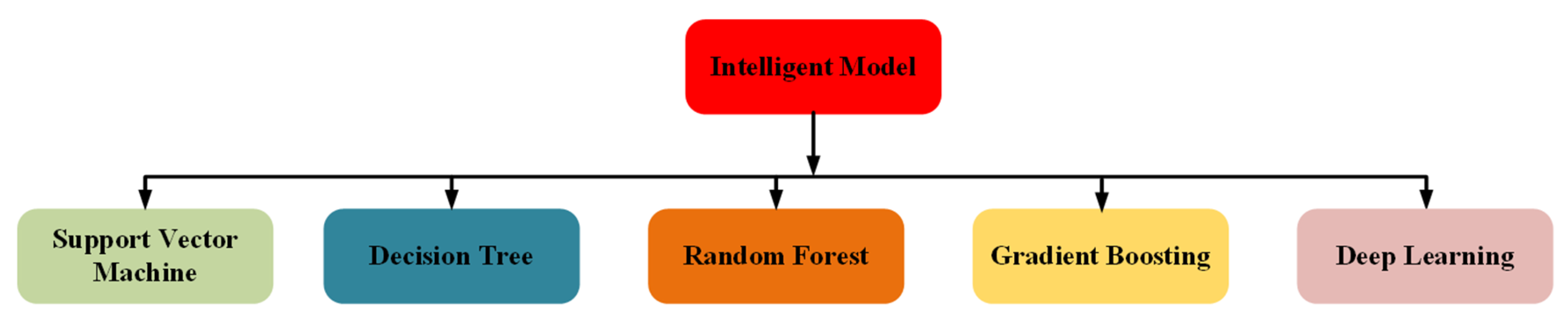
3.2. Intelligent Models

Intelligent models in short-term load forecasting (STLF) refer to forecasting techniques that leverage advanced computational methods, such as artificial intelligence, machine learning, and optimization algorithms, to predict the electricity load in the short term. These models are designed to capture complex patterns, nonlinear relationships, and dependencies in the load data, leading to improved forecasting accuracy and reliability [57]. Figure 7 displays some of the main intelligent models used in STLF.

3.2.1. Support Vector Machine

One important ML model for STLF is the support vector machine (SVM), a supervised learning model that can handle linear and nonlinear relationships between the load and other factors that influence the load. SVMs can control various predictor variables, including categorical variables and interaction terms [58]. They can also handle noisy data using a kernel function to map it to a higher-dimensional space. SVMs have been used successfully in power system applications to forecast the load based on temperature, humidity, and time of day. In the context of short-term load forecasting (STLF), SVMs can be employed to predict electricity load or demand for a specific upcoming period, usually ranging from a few hours to a week ahead. The primary goal of an SVM is to find the optimal hyperplane that maximally separates two classes of data points. In a two-dimensional space, a hyperplane is a line that separates the data into two classes. It is a hyperplane (a subspace with one dimension less than the containing space) in higher-dimensional spaces. The margin is the distance between the hyperplane and the closest data points from both classes. These closest points are called support vectors, which “support” the hyperplane. The objective of an SVM is to maximize the margin while correctly classifying the data points. Given a dataset of labeled data points (x_i, y_i), where x_i ∈ Rⁿ is the feature vector, and y_i ∈ {−1, 1} is the class label, the hyperplane can be defined as [59]:

$$w·x+b=0$$

(21)

Here, w is the weight vector, x is the input feature vector, and b is the bias term. The dot product (w·x) measures the projection of x onto the direction of w. The goal is to find the optimal w and b that maximize the margin between the two classes.

The decision function for classification is

$$f\left(x\right)=sign\left(w·x+b\right)$$

(22)

where sign(.) is the signum function that outputs the class label based on the sign of its argument.

The margin for each data point can be computed as:

$$y_i\left(w·x_i+b\right)$$

(23)

where:

• y_i is the true label of the i-th data point; in the binary classification case, it takes the value of either −1 or +1.
• w is the weight vector, which is orthogonal to the decision boundary (hyperplane).
• x_i is the feature vector of the i-th data point.
• b is the bias term, which shifts the decision boundary away from the origin.
• w⋅x_i is the dot product between the weight vector w and the feature vector x_i, which represents the projection of x_i onto the weight vector.

The objective of the SVM is to maximize the margin while ensuring that all data points are correctly classified. The margin can be maximized by minimizing the norm of the weight vector, ‖w‖. This is because the distance between the hyperplane and the closest data point is inversely proportional to ‖w‖.

$$Margin=\raisebox{1ex}{$1$}\!\left/ \!\raisebox{-1ex}{$\Vert w\Vert $}\right.$$

(24)

The optimization problem for an SVM can be formulated as a constrained optimization problem:

$$Minimize:\frac{1}{2}\ast \Vert w{\Vert }^2$$

(25)

subject to: y_i(w·x_i + b) ≥ 1, for all i = 1, …, N.

Here, N is the number of data points in the dataset.

This is a convex quadratic programming problem with linear constraints. We can use the Lagrange multipliers method to solve this problem, which leads to the dual problem. The dual problem is a more convenient form for solving the SVM optimization problem, especially for nonlinear cases when using kernel functions [60].

The step-wise working of STLF is shown in Figure 8 and explained below.

• The first step involves collecting historical electricity load data and relevant exogenous variables such as weather data, day of the week, and time of the day. These data are cleaned and preprocessed to remove any inconsistencies, outliers, or missing values, and are often normalized or standardized to improve the performance of the SVM.
• Next, the most relevant features are selected for the forecasting task. This step is crucial, as irrelevant or redundant features can negatively impact the model’s performance. Techniques such as recursive feature elimination (RFE), correlation analysis, or principal component analysis (PCA) can be applied to identify the most significant features of the problem.
• The SVM model is trained with the preprocessed data and the selected features. SVMs aim to find the optimal hyperplane that best separates the data into different classes or categories. In the case of STLF, it is a regression problem, so the model will learn to predict continuous values for the electricity load. To do this, the SVM algorithm uses kernel functions (such as linear, polynomial, or radial basis functions) to transform the input data into a higher-dimensional space, making finding the optimal separating hyperplane easier.
• To ensure the SVM model performs well on unseen data, it is validated using techniques such as cross-validation. During this process, the dataset is divided into training and validation subsets, with the model being trained on one subset and tested on the other. This helps to assess the model’s performance and generalizability. Moreover, hyperparameters such as the cost parameter (C), kernel type, and kernel parameters are tuned to find the best combination for the specific STLF problem.
• After training and tuning the SVM model, it is tested on an unseen dataset to evaluate its forecasting accuracy. Performance metrics such as mean absolute error (MAE), mean squared error (MSE), or mean absolute percentage error (MAPE) are used to quantify the model’s predictive capabilities.
• Once the SVM model has been trained, validated, and tested, it can be used to make short-term load forecasts based on new input data. The model takes in the relevant features for the desired forecasting period and outputs the predicted electricity load.

3.2.2. Decision Tree

Another ML model for STLF is the decision tree (DT), a supervised learning model that can handle both categorical and continuous predictor variables [60]. DTs work by partitioning the predictor variables into subsets based on their relevance to the load and constructing a decision tree that can be used to predict the load based on the predictor variables. DTs have been used successfully in power system applications to forecast the load based on weather conditions, occupancy, and time of day. The key concepts in decision trees are [61]:

Node: A decision tree consists of nodes, where each node represents a decision or a split based on a feature’s value [62].

Leaf: The terminal nodes of the tree, where no further splitting occurs, are called leaves. They represent the final decision or output for a given input.

Split criterion: The choice of feature and the split value at each node is based on a split criterion, which aims to maximize the homogeneity (purity) of the resulting child nodes.

For a classification task, two common split criteria are:

• Gini impurity: Gini impurity measures a node’s impurity (class mixture), with lower values indicating higher purity [63]. The Gini impurity for a node with class probabilities p_i is:

$$Gini impurity=1-\Sigma \left({\pi }^2\right)$$

(26)

b.

Information gain: Information gain is based on entropy, which measures the randomness or uncertainty in a set. The entropy for a node with class probabilities π is:

$$Entropy=-\Sigma (p_i\ast {\log }_2\left(\pi \right))$$

(27)

The information gain is the difference in entropy before and after the split:

Information gain = Entropy(parent) − weighted sum(Entropy(children))

(28)

The goal is to maximize the information gain, which leads to more homogeneous child nodes.

For a regression task, the common split criterion is mean squared error (MSE). The MSE measures the average squared difference between the actual and predicted target values [64]. The objective is to minimize the MSE for each split.

$$MSE=\frac{1}{N}\ast \Sigma (y_i-{\widehat{y_i})}^2$$

(29)

Figure 9 shows the working of a decision tree algorithm, and this process is explained below.

• The first step involves collecting historical electricity load data and relevant exogenous variables such as weather data, day of the week, and time of the day. These data are cleaned and preprocessed to remove any inconsistencies, outliers, or missing values. Feature scaling is generally not required for decision trees, as they are less sensitive to the scale of input features.
• The most relevant features for the forecasting task are selected to ensure that irrelevant or redundant features do not negatively impact the model. Techniques such as recursive feature elimination (RFE), correlation analysis, or information gain can be applied to identify the most significant features of the problem.
• With the preprocessed data and selected features, the decision tree model is trained. The algorithm recursively splits the data into subsets based on the input features’ values to minimize the impurity of the resulting subsets. For a regression task such as STLF, the impurity can be measured using criteria such as mean squared error (MSE). The algorithm splits the data until a stopping criterion is reached, such as a maximum tree depth or a minimum number of samples in a leaf node.
• Decision trees can be prone to overfitting, especially when they grow too deep. To address this issue, the model is validated using techniques such as cross-validation. The dataset is divided into training and validation subsets, with the model being trained on one subset and tested on the other. This method helps assess the model’s performance and generalizability. Additionally, pruning techniques, such as cost-complexity or reduced-error pruning, can simplify the tree and reduce overfitting.
• After training and pruning the decision tree model, it is tested on an unseen dataset to evaluate its forecasting accuracy. Performance metrics such as mean absolute error (MAE), mean squared error (MSE), or mean absolute percentage error (MAPE) are used to quantify the model’s predictive capabilities [65].
• Once the decision tree model has been trained, validated, and tested, it can make short-term load forecasts based on new input data. The model takes in the relevant features for the desired forecasting period and traverses the tree from the root node to a leaf node, following the decision rules at each split. The output at the leaf node is the predicted electricity load.

3.2.3. Random Forest and Gradient Boosting

Random forest (RF) is an extension of DTs that can handle overfitting and improve the accuracy of the load forecasts. RFs construct multiple decision trees using bootstrap samples of the training data and averaging the predictions of the individual trees [66]. RFs have been used successfully in power system applications to forecast the load based on temperature, humidity, and solar radiation. Figure 10 shows the working of a random forest algorithm. The m features are selected from the incoming instances. The different numbers of trees are made, leading to unique prediction classes. The majority vote determines the final class [66].

Gradient boosting (GB) is an ensemble ML model that can improve the accuracy of load forecasts [67]. GB works by sequentially adding decision trees to the model, which corrects the errors of the previous trees, resulting in a final model that can capture the nonlinear relationships between the load and other factors that influence the load. GB has been used successfully in power system applications to forecast the load based on weather conditions, occupancy, and time of day [68]. Figure 11 is a block diagram of the gradient boosting algorithm. The data training determines the weak learners used to make a more accurate prediction.

The step-wise working of random forest and gradient boosting algorithms is below.

• The first step involves collecting historical electricity load data and relevant exogenous variables such as weather data, day of the week, and time of the day. These data are cleaned and preprocessed to remove inconsistencies, outliers, or missing values. Feature scaling is generally not required for random forest as decision trees, its base learners, are less sensitive to the scale of input features.
• The most relevant features for the forecasting task are selected to ensure that irrelevant or redundant features do not negatively impact the model. Although random forest has an inherent ability to handle many features and automatically estimate feature importance, using domain knowledge or techniques such as recursive feature elimination (RFE) and correlation analysis can help further improve model performance.
• With the preprocessed data and selected features, the random forest model is trained. The algorithm creates multiple decision trees, and each tree is trained on a different bootstrap sample of the original dataset (sampling with replacement). Additionally, a random subset of features is considered at each split in the tree construction process, which introduces further diversity among the trees and reduces overfitting.
• The cross-validation technique ensures that the random forest model performs well on unseen data. The dataset is divided into training and validation subsets, with the model being trained on one subset and tested on the other. This process helps assess the model’s performance and generalizability.
• Random forest has several hyperparameters, such as the number of trees (n_estimators), the maximum depth of the trees, and the minimum number of samples required to split a node. These hyperparameters can be tuned using techniques such as grid or random search and cross-validation to find the best combination for the specific STLF problem.
• Once the random forest model has been trained, validated, and tested, it can make short-term load forecasts based on new input data. The model takes in the relevant features for the desired forecasting period and produces a prediction from each decision tree. The final prediction is the average of the individual tree predictions, which provides a more accurate and stable forecast.

3.2.4. Multilayer Perceptron Model

A multilayer perceptron (MLP) is an artificial neural network consisting of multiple layers of interconnected nodes, also known as neurons or perceptrons. It is widely used in supervised learning tasks, such as classification and regression. An MLP is shown in Figure 12, it has the following components [69]:

• Input layer: This is the first layer of the MLP model, receiving the input data (e.g., numbers, images, and text). Each node in this layer corresponds to a single input data feature.
• Hidden layers: These are the layers between the input and output layers. They consist of neurons that learn to represent and process the data. The more hidden layers and neurons per layer, the more complex patterns the model can learn.
• Output layer: The last layer in the MLP model produces the final results or predictions. The number of nodes in this layer depends on the problem one is trying to solve. For example, if images are classified into ten categories, the output layer will have ten nodes.
• Neurons: Each neuron in the MLP model receives input from other neurons, processes it using an activation function, and sends the output to other neurons in the next layer. The activation function introduces non-linearity, which enables the MLP to learn complex patterns in the data.
• Weights and biases: Each connection between neurons has a weight that determines the strength of the association. The weights are adjusted during training to minimize the difference between the predicted and actual values. Biases are additional constants that help shift the activation function, improving the model’s learning ability.
• Training: MLP models are trained using a backpropagation algorithm, which adjusts the weights and biases by minimizing the error between the predicted and actual values. The process is iterative, involving multiple passes through the data to fine-tune the model.
• Loss function: This is a measure of how well the MLP model is performing. A lower value indicates better performance. During training, the goal is to minimize the loss of function.

Mathematically, the output of a neuron can be represented as [66]:

$$a_j=f\left(\sum (w_{ij}\ast x_i\right)+b_j)$$

(30)

where:

• a_j is the output (activation) of neuron j;
• f is the activation function;
• w_ij is the weight connecting input i to neuron j;
• x_i is the input value for input i;
• b_j is the bias term for neuron j.

For each layer in the MLP, this equation can be applied in a matrix form:

$$A=f\left(WX+B\right)$$

(31)

where:

• A is the activation matrix (each column represents the activation of a neuron);
• f is the activation function applied element-wise;
• W is the weight matrix;
• X is the input matrix (each column represents an input feature vector);
• B is the bias matrix.

After computing the activations for all layers, the output layer produces the final prediction. For classification tasks, a softmax function is typically used in the output layer to convert the activations into probabilities:

softmax(a_i) = exp(a_i)/Σ(exp(a_j))

(32)

where:

• a_i is the activation of output neuron i,
• a_j is the activation of output neuron j,

softmax(a_i) is the probability for class i.

3.2.5. Deep Learning Models

Deep learning (DL) is a class of ML models that can capture complex nonlinear relationships between the load and other factors that influence the load [70]. DL models consist of multiple layers of interconnected nodes that process and transmit information through weighted connections [71]. One popular DL model for STLF is the convolutional neural network (CNN), which can capture the spatial and temporal patterns in the load data. CNNs have been used successfully in power system applications to forecast the load based on weather conditions, occupancy, and time of day [72]. Another critical DL model for STLF is the recurrent neural network (RNN), which can capture the temporal dependencies in the load data. RNNs use feedback connections to allow information to be passed from one time step to the next, enabling the model to capture the dynamics of the load over time. One type of RNN is the long short-term memory (LSTM) network, which is well-suited for STLF as it can capture both short-term and long-term dependencies in the load data [73].

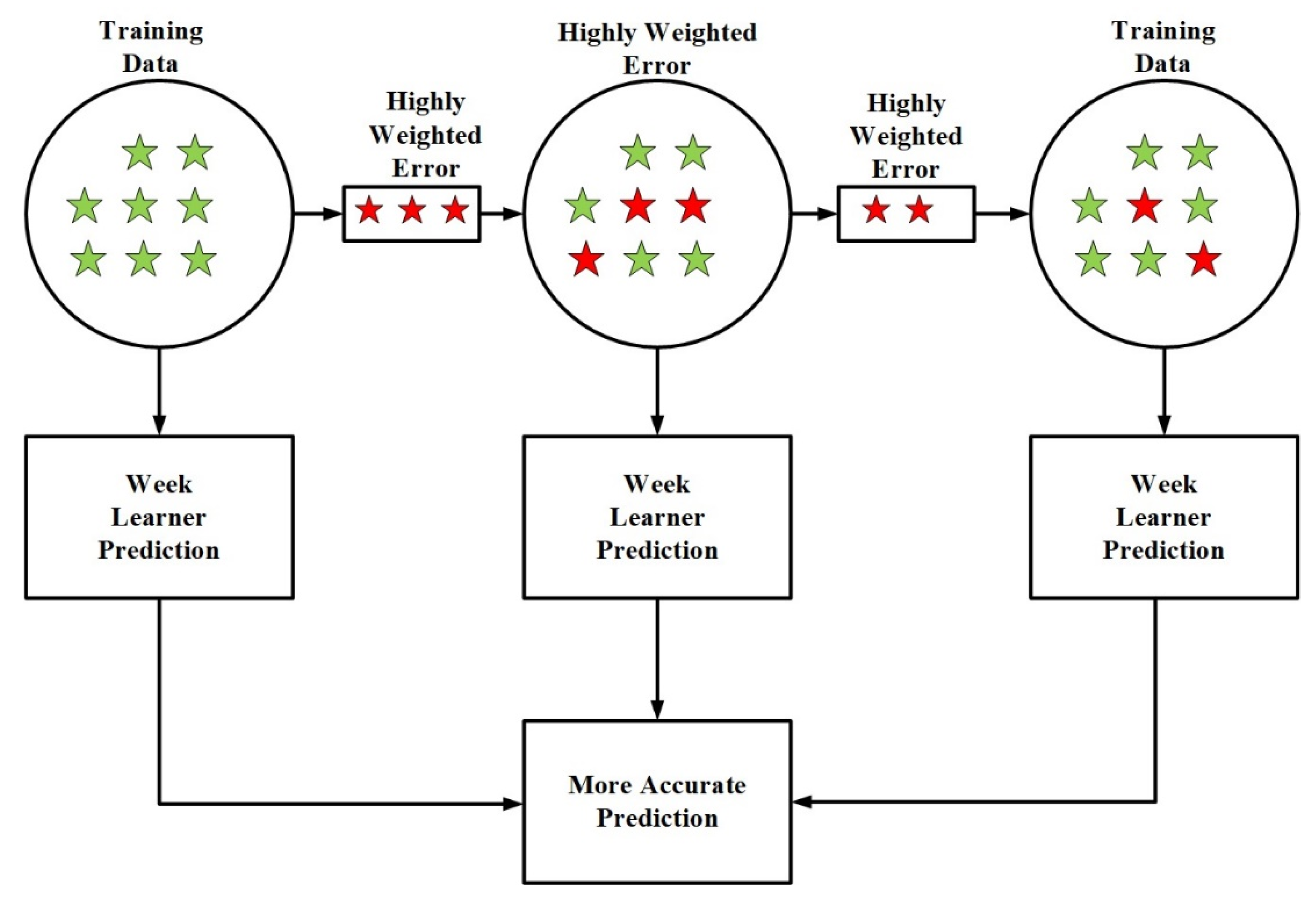
3.2.6. Ensemble Models

Ensemble models are machine learning models that combine multiple models’ predictions to produce a final prediction [74]. The basic idea behind ensemble models is to use the strengths of different models and combine their predictions to create a more accurate and robust forecast. Ensemble models can be used in various machine learning tasks, including classification, regression, and clustering [75]. One of the main advantages of ensemble models is their ability to reduce variance and overfitting. Variance is a measure of how much the predictions of the models in the ensemble vary from each other. Overfitting occurs when a model is too complex and fits the training data too closely, leading to poor performance on new, unseen data. Ensemble models can reduce variance and overfitting by combining the predictions of multiple models, thereby reducing the overall variance and producing a more robust forecast [76]. One of the main disadvantages of ensemble models is their complexity. Ensemble models can be more complex to implement and interpret than single models and may require more computational resources [77].

Additionally, the performance of ensemble models can depend on the specific combination of models used, and finding the optimal combination can be challenging. Another disadvantage of ensemble models is their sensitivity to the quality of the models in the ensemble [78]. Poor-quality models can negatively affect ensemble models, such as overfitting or underfitting the data. It is essential to carefully select the models in the ensemble and ensure that they are high quality. Several techniques for creating ensemble models include bagging, boosting, and stacking shown in Figure 13. Each technique has its strengths and limitations, and the choice of method depends on the specific application and dataset.

• Bragging.

Bagging, or bootstrap aggregating, is a technique that involves training multiple models on different subsets of the training data and then combining their predictions using a weighted average. Bagging can be used with any model and can reduce variance and overfitting. The basic idea behind bagging is to create multiple copies of the original dataset, each with a different subset of the data [79]. The models are then trained on each of these copies, combining their predictions to produce a final prediction. By combining the predictions of multiple models, bagging can produce a more accurate and robust forecast.

B.

Boosting.

Boosting is a technique that involves training multiple models sequentially, with each model focusing on the examples that the previous model misclassified. Boosting can improve the accuracy of the forecast but may be more prone to overfitting than bagging. The basic idea behind boosting is to start with a simple model and then sequentially add more complex models that focus on the examples that the previous model misclassified [80]. The models are combined using a weighted sum, with weights that depend on their accuracy. By focusing on the examples that the previous model misclassified, boosting can produce a more accurate and robust forecast.

C.

Stacking.

Stacking, or stacked generalization, is a technique that involves training multiple models on the training data and then using their predictions as input to a higher-level model. The higher-level model learns to combine the predictions of the lower-level models to produce a final prediction. Stacking can improve the accuracy and robustness of the forecast but may be more complex to implement and interpret than bagging or boosting [81]. The basic idea behind stacking is to train multiple models on the training data and then use their predictions as input to a higher-level model. The higher-level model learns to combine the predictions of the lower-level models to produce a final prediction. By combining the predictions of multiple models, stacking can create a more accurate and robust forecast.

3.3. Hybrid Models

Hybrid models combine the advantages of both statistical and machine learning models. The most used hybrid models for STLF are ARIMA–SVR and ES–ANN. ARIMA–SVR integrates the ARIMA and SVR models and can capture the temporal patterns and nonlinear relationships of load demand [82]. ES–ANN combines ES and ANN models and can capture the seasonal and nonlinear patterns of load demand. Hybrid models can improve the accuracy and interpretability of STLF models for power system applications. However, they require more computational resources than statistical models and may be more challenging to implement than machine learning models [83]. Hybrid models, which combine different modeling techniques, have been proposed to improve the accuracy of load forecasts [84]. The following are some of the essential hybrid models:

3.3.1. ARIMA–ANN Hybrid Model

The autoregressive integrated moving average (ARIMA) model is a classical time-series forecasting method that captures linear dependencies in the data. Artificial neural networks (ANNs) are capable of learning complex nonlinear patterns. By combining the linear forecasting ability of ARIMA with the nonlinear forecasting ability of ANNs, this hybrid model can capture both linear and nonlinear dependencies in the load data, resulting in improved STLF accuracy [85].

3.3.2. Wavelet-Transform-Based Hybrid Models

Wavelet transform is a technique that decomposes a time series into different frequency components, which can be analyzed separately. The high-frequency components represent noise and sudden changes, while low-frequency components capture the underlying trends. Wavelet transform can be combined with various forecasting techniques, such as ANN, support vector machines (SVM), or long short-term memory (LSTM) networks, to create a hybrid model. It can handle the frequency components separately, leading to improved forecast accuracy [86].

3.3.3. EEMD–ANN Hybrid Model

The ensemble empirical mode decomposition (EEMD) is an advanced signal processing technique that decomposes a non-stationary time series into a set of intrinsic mode functions (IMFs). Combining EEMD with ANN allows this hybrid model to handle non-stationary and nonlinear load data more effectively. The EEMD preprocesses the load data by extracting the IMFs, and the ANN is trained on these IMFs to generate forecasts. The forecasts are then combined to produce the final STLF [87].

3.3.4. Fuzzy-Logic-Based Hybrid Models

Fuzzy logic is a mathematical approach that deals with uncertainty and imprecision in data. It can be combined with other forecasting techniques such as ANN, SVM, or regression models to create a hybrid model that handles the uncertainty in load data more effectively. Fuzzy logic can preprocess the input data, model the uncertainties in the forecasting model, or fuse the forecasts from different models [88].

3.3.5. Deep-Learning-Based Hybrid Models

Deep learning techniques, such as convolutional neural networks (CNN) and LSTMs, have shown great potential in STLF due to their ability to learn hierarchical and temporal features in the data. These deep learning models can be combined with other forecasting techniques, such as statistical models, wavelet transform, or fuzzy logic, to create hybrid models that leverage the strengths of both approaches for improved STLF accuracy [89].

3.4. Performance Comparison of STLF Models

The performance of STLF models depends on various factors, such as the size and quality of the data, the forecasting horizon, and the complexity of the underlying relationships between the variables. Intelligent models outperform statistical models, and hybrid models outperform both statistical and intelligent models [90]. However, the models’ relative performance can vary depending on the application and dataset. For example, statistical models may perform well when the data are stationary and linear and when limited data are available. Intelligent models may perform well when the data are nonlinear and non-stationary and when a large amount of data is available. Hybrid models may perform well when there are both linear and nonlinear relationships between the variables and when the data are noisy or missing.

Table 2. Performance comparison of STLF Models.

Refs.	Model	Contributions	Applications	Limitations
[91]	ARIMA	Suitable for modeling time series data with trend and seasonality	Forecasting of various economic and financial data, weather forecasting, and sales forecasting	Assumes stationarity and requires careful selection of model parameters
[92]	SARIMA	Incorporates seasonal factors into ARIMA model	Forecasting of time series data with seasonal patterns, such as sales data during holiday seasons	Requires careful selection of model parameters
[93]	Exponential Smoothing	Simple yet effective method for time series forecasting	Used in various industries, such as finance, supply chain management, and marketing	Assumes no trend or seasonality in data
[94]	Generalized Linear Model	Extends linear regression to accommodate non-normal response variables	Used in various fields, such as medical research, environmental science, and social sciences	Assumes linearity between predictors and response variable
[95]	Support Vector Machine	Nonlinear classification and regression method	Used in various fields, such as finance, biology, and image recognition	Requires careful selection of model parameters
[96]	Decision Tree	Non-parametric method for classification and regression	Used in various fields, such as finance, marketing, and healthcare	Prone to overfitting and requires careful selection of hyperparameters
[97]	Random Forest	Ensemble method that uses multiple decision trees for classification and regression	Used in various fields, such as finance, marketing, and healthcare	Prone to overfitting and requires careful selection of hyperparameters
[98]	Gradient Boosting	Ensemble method that uses multiple weak learners to improve predictions	Used in various fields, such as finance, healthcare, and image recognition	Prone to overfitting and requires careful selection of hyperparameters
[99]	Deep Learning	Neural-network-based models for complex data analysis	Used in various fields, such as image recognition, natural language processing, and speech recognition	Requires large amounts of training data and computational resources
[100]	Ensemble Methods	Combine multiple models to improve prediction accuracy	Used in various fields, such as finance, marketing, and healthcare	Requires careful selection of models and hyperparameters
[101]	Multilayer Perceptron	Neural-network-based models for classification and regression	Used in various fields, such as finance, healthcare, and image recognition	Prone to overfitting and requires careful selection of hyperparameters
[102]	Hybrid Models	Combine multiple models or methods to improve prediction accuracy	Used in various fields, such as finance, marketing, and healthcare	Requires careful selection of models and hyperparameters

summarizes the findings.

4. The Road Ahead

Short-term load forecasting (STLF) is critical in the energy industry. It enables power system operators to make informed decisions about resource allocation, power generation, and grid stability. Over the years, numerous STLF models have been developed and evaluated, but there is still room for improvement. Some potential future research directions in the development of STLF models are shown in Figure 14.

• Incorporating new data sources: Traditional STLF models rely on historical load, weather, and calendar data as input features. However, the availability of new data sources, such as social media data and smart meter data, presents an opportunity to develop more accurate and robust STLF models [103]. Future studies can examine the application of machine learning algorithms to identify the most relevant data sources for predicting electricity demand and how best to incorporate these data sources into STLF models.
• Development of hybrid models: Hybrid models combine different models or techniques to address specific challenges or achieve specific goals. Hybrid models can combine traditional STLF models with models for predicting renewable energy production or demand-side management (DSM) models [104]. Future research can examine the development of more advanced hybrid models that can handle multiple input features, uncertainty quantification, and other challenges in STLF modeling.
• Integration of advanced machine learning techniques: Advanced machine learning techniques, such as deep learning and reinforcement learning, have shown great potential in improving the accuracy of STLF models. Deep learning techniques can automatically learn complex patterns and relationships in the data, while reinforcement learning can learn to optimize actions based on feedback from the environment [105]. Future work can investigate the creation of more sophisticated machine learning models that can manage vast volumes of data, combine numerous input features, and adjust to shifting energy system conditions.
• Handling of non-stationary and nonlinear load data: Traditional STLF models assume that the load data is stationary and linear. However, the load data can be non-stationary and nonlinear due to changes in consumer behavior, the introduction of new technologies, and other factors [106]. Future research can explore the development of STLF models that can handle non-stationary and nonlinear load data, either through advanced machine learning techniques or more flexible statistical models.
• Integration of probabilistic forecasting: Probabilistic forecasting measures uncertainty around the point forecast. It can help power system operators make more informed decisions in the face of uncertainty [107]. Future work can support the development of STLF models that can provide point forecasts and uncertainty estimates, such as prediction intervals or probabilistic forecasts. These uncertainty estimates can help to identify potential risks and improve the overall reliability of the power system.
• Integration of online learning: Online learning is a type of machine learning that can adapt to changing conditions in the energy system in real-time [108]. Online learning algorithms can learn from new data as it becomes available and adjust the forecast accordingly. Future studies may look toward creating STLF models that employ online learning algorithms to increase forecast precision and timeliness [109].
• Development of interpretable models: Interpretable models are models that can provide insights into the factors that are driving the forecast. Interpretable models can help power system operators understand the underlying patterns and relationships in the data and make more informed decisions about resource allocation and power generation [110]. Additional studies may examine the creation of STLF models that are easier to understand, either via the use of advanced machine learning techniques or more straightforward statistical models [111].
• Integration of ensemble methods: Ensemble methods, such as bagging and boosting, have shown great potential in improving the accuracy and robustness of STLF models. Ensemble methods can combine and overfit them and be used to select the best model for a given dataset [112]. Future work could investigate the creation of more sophisticated ensemble models capable of handling various input features, uncertainty quantification, and other difficulties in STLF modeling [113].
• Handling of data quality issues: Data quality issues, such as missing data, outliers, and measurement errors, can have a significant impact on the accuracy of STLF models [114]. Future studies could assist in creating STLF models that can deal with problems with data quality by prediction models or more sophisticated statistical models that can directly deal with missing data.
• Integration of domain knowledge: Domain knowledge, such as knowledge about consumer behavior, the energy system, and the environment, can provide valuable insights into the factors driving electricity demand [115]. Future studies can create STLF models that incorporate domain knowledge into the modeling process, either through expert systems or sophisticated machine learning methods that can add domain knowledge as different input characteristics.
• Development of adaptive models: The energy system constantly changes, and the factors driving the electricity demand can vary over time [116]. Future studies may examine the creation of STLF models that can modify their predictions in response to changing energy system conditions, either using online learning algorithms or more adaptable statistical models.
• Handling multiple time scales: The electricity demand can exhibit patterns on various time scales, such as daily, weekly, and seasonal patterns [117]. Future studies can develop STLF models that can handle multiple time scales by combining models trained on various time scales or utilizing more sophisticated machine-learning methods.
• Integration of uncertainty information: Uncertainty information, such as information about input data reliability or model accuracy, can provide valuable insights into the quality of the forecast [118]. Future studies may explore creating STLF models that can incorporate uncertainty data into the modeling process through probabilistic models or more sophisticated statistical models that can calculate forecast uncertainty [119].
• Development of models for distributed energy resources: The increasing use of distributed energy resources, such as rooftop solar panels and energy storage systems, has introduced new challenges for STLF models [120]. Future studies may develop STLF models that can account for distributed energy resources, either through models that forecast the production of renewable energy or models that forecast the effects of distributed energy resources on electricity consumption [121,122].

5. Conclusions

STLF models are an essential component of the energy industry, as they enable power system operators to make informed decisions about resource allocation, power generation, and grid stability. This review article has presented an overview of the state-of-the-art STLF models for power system applications, including statistical, intelligent, and hybrid models. These models have their strengths and limitations. The choice of model depends on various factors, such as the size and quality of the data, the forecasting horizon, and the complexity of the underlying relationships between the variables. Power system operators should carefully evaluate the performance of different models and consider these factors when selecting the most appropriate model for their application. The development of STLF models is an ongoing research area, and future advances in machine learning, data analytics, and computational resources are expected to improve the accuracy and robustness of STLF models.

References

1. Cheng, L.; Yu, T. A new generation of AI: A review and perspective on machine learning technologies applied to smart energy and electric power systems. Int. J. Energy Res. 2019, 43, 1928–1973. [Google Scholar] [CrossRef]
2. Ding, Y.; Zhu, Y.; Feng, J.; Zhang, P.; Cheng, Z. Interpretable spatio-temporal attention LSTM model for flood forecasting. Neurocomputing 2020, 403, 348–359. [Google Scholar] [CrossRef]
3. Zakaria, A.; Ismail, F.B.; Lipu, M.H.; Hannan, M. Uncertainty models for stochastic optimization in renewable energy applications. Renew. Energy 2020, 145, 1543–1571. [Google Scholar] [CrossRef]
4. Fu, H.; Baltazar, J.-C.; Claridge, D.E. Review of developments in whole-building statistical energy consumption models for commercial buildings. Renew. Sustain. Energy Rev. 2021, 147, 111248. [Google Scholar] [CrossRef]
5. Lu, S.; Li, Q.; Bai, L.; Wang, R. Performance predictions of ground source heat pump system based on random forest and back propagation neural network models. Energy Convers. Manag. 2019, 197, 111864. [Google Scholar] [CrossRef]
6. Ganaie, M.; Hu, M.; Malik, A.; Tanveer, M.; Suganthan, P. Ensemble deep learning: A review. Eng. Appl. Artif. Intell. 2022, 115, 105151. [Google Scholar] [CrossRef]
7. Altan, A.; Karasu, S.; Zio, E. A new hybrid model for wind speed forecasting combining long short-term memory neural network, decomposition methods and grey wolf optimizer. Appl. Soft Comput. 2021, 100, 106996. [Google Scholar] [CrossRef]
8. Alexander, M.; Beushausen, H. Durability, service life prediction, and modelling for reinforced concrete structures—Review and critique. Cem. Concr. Res. 2019, 122, 17–29. [Google Scholar] [CrossRef]
9. Kurani, A.; Doshi, P.; Vakharia, A.; Shah, M. A Comprehensive Comparative Study of Artificial Neural Network (ANN) and Support Vector Machines (SVM) on Stock Forecasting. Ann. Data Sci. 2023, 10, 183–208. [Google Scholar] [CrossRef]
10. Dagoumas, A.S.; Koltsaklis, N.E. Review of models for integrating renewable energy in the generation expansion planning. Appl. Energy 2019, 242, 1573–1587. [Google Scholar] [CrossRef]
11. Zhang, R.; Chen, Z.; Chen, S.; Zheng, J.; Büyüköztürk, O.; Sun, H. Deep long short-term memory networks for nonlinear structural seismic response prediction. Comput. Struct. 2019, 220, 55–68. [Google Scholar] [CrossRef]
12. Lindberg, K.B.; Seljom, P.; Madsen, H.; Fischer, D.; Korpås, M. Long-term electricity load forecasting: Current and future trends. Util. Policy 2019, 58, 102–119. [Google Scholar] [CrossRef]
13. Koponen, P.; Ikäheimo, J.; Koskela, J.; Brester, C.; Niska, H. Assessing and Comparing Short Term Load Forecasting Performance. Energies 2020, 13, 2054. [Google Scholar] [CrossRef]
14. Trierweiler Ribeiro, G.; Cocco Mariani, V.; dos Santos Coelho, L. Enhanced ensemble structures using wavelet neural networks applied to short-term load forecasting. Eng. Appl. Artif. Intell. 2019, 82, 272–281. [Google Scholar] [CrossRef]
15. Moradzadeh, A.; Moayyed, H.; Zakeri, S.; Mohammadi-Ivatloo, B.; Aguiar, A.P. Deep Learning-Assisted Short-Term Load Forecasting for Sustainable Management of Energy in Microgrid. Inventions 2021, 6, 15. [Google Scholar] [CrossRef]
16. Almalaq, A.; Edwards, G. A Review of Deep Learning Methods Applied on Load Forecasting. In Proceedings of the 2017 16th IEEE International Conference on Machine Learning and Applications (ICMLA), Cancun, Mexico, 18–21 December 2017; pp. 511–516. [Google Scholar] [CrossRef]
17. Li, L.-L.; Zhao, X.; Tseng, M.-L.; Tan, R.R. Short-term wind power forecasting based on support vector machine with improved dragonfly algorithm. J. Clean. Prod. 2020, 242, 118447. [Google Scholar] [CrossRef]
18. Carvalho, T.P.; Soares, F.A.A.M.N.; Vita, R.; Francisco, R.D.P.; Basto, J.P.; Alcalá, S.G.S. A systematic literature review of machine learning methods applied to predictive maintenance. Comput. Ind. Eng. 2019, 137, 106024. [Google Scholar] [CrossRef]
19. Chen, J.; Ran, X. Deep Learning with Edge Computing: A Review. Proc. IEEE 2019, 107, 1655–1674. [Google Scholar] [CrossRef]
20. Nespoli, A.; Ogliari, E.; Leva, S.; Pavan, A.M.; Mellit, A.; Lughi, V.; Dolara, A. Day-Ahead Photovoltaic Forecasting: A Comparison of the Most Effective Techniques. Energies 2019, 12, 1621. [Google Scholar] [CrossRef]
21. Mahzarnia, M.; Moghaddam, M.P.; Baboli, P.T.; Siano, P. A Review of the Measures to Enhance Power Systems Resilience. IEEE Syst. J. 2020, 14, 4059–4070. [Google Scholar] [CrossRef]
22. Ahmad, T.; Zhang, D.; Huang, C.; Zhang, H.; Dai, N.; Song, Y.; Chen, H. Artificial intelligence in sustainable energy industry: Status Quo, challenges and opportunities. J. Clean. Prod. 2021, 289, 125834. [Google Scholar] [CrossRef]
23. Ruano, A.; Hernandez, A.; Ureña, J.; Ruano, M.; Garcia, J. NILM Techniques for Intelligent Home Energy Management and Ambient Assisted Living: A Review. Energies 2019, 12, 2203. [Google Scholar] [CrossRef]
24. Mohandes, B.; El Moursi, M.S.; Hatziargyriou, N.D.; El Khatib, S. A Review of Power System Flexibility with High Penetration of Renewables. IEEE Trans. Power Syst. 2019, 34, 3140–3155. [Google Scholar] [CrossRef]
25. Liu, Z.; Jiang, P.; Zhang, L.; Niu, X. A combined forecasting model for time series: Application to short-term wind speed forecasting. Appl. Energy 2020, 259, 114137. [Google Scholar] [CrossRef]
26. Laib, O.; Khadir, M.T.; Mihaylova, L. Toward efficient energy systems based on natural gas consumption prediction with LSTM Recurrent Neural Networks. Energy 2019, 177, 530–542. [Google Scholar] [CrossRef]
27. Boukerche, A.; Wang, J. Machine Learning-based traffic prediction models for Intelligent Transportation Systems. Comput. Netw. 2020, 181, 107530. [Google Scholar] [CrossRef]
28. Sharifzadeh, M.; Sikinioti-Lock, A.; Shah, N. Machine-learning methods for integrated renewable power generation: A comparative study of artificial neural networks, support vector regression, and Gaussian Process Regression. Renew. Sustain. Energy Rev. 2019, 108, 513–538. [Google Scholar] [CrossRef]
29. Qiao, W.; Huang, K.; Azimi, M.; Han, S. A Novel Hybrid Prediction Model for Hourly Gas Consumption in Supply Side Based on Improved Whale Optimization Algorithm and Relevance Vector Machine. IEEE Access 2019, 7, 88218–88230. [Google Scholar] [CrossRef]
30. Fan, C.; Wang, J.; Gang, W.; Li, S. Assessment of deep recurrent neural network-based strategies for short-term building energy predictions. Appl. Energy 2019, 236, 700–710. [Google Scholar] [CrossRef]
31. Hossain, E.; Khan, I.; Un-Noor, F.; Sikander, S.S.; Sunny, S.H. Application of Big Data and Machine Learning in Smart Grid, and Associated Security Concerns: A Review. IEEE Access 2019, 7, 13960–13988. [Google Scholar] [CrossRef]
32. Blaga, R.; Sabadus, A.; Stefu, N.; Dughir, C.; Paulescu, M.; Badescu, V. A current perspective on the accuracy of incoming solar energy forecasting. Prog. Energy Combust. Sci. 2019, 70, 119–144. [Google Scholar] [CrossRef]
33. Wang, F.; Xuan, Z.; Zhen, Z.; Li, K.; Wang, T.; Shi, M. A day-ahead PV power forecasting method based on LSTM-RNN model and time correlation modification under partial daily pattern prediction framework. Energy Convers. Manag. 2020, 212, 112766. [Google Scholar] [CrossRef]
34. Zahid, M.; Ahmed, F.; Javaid, N.; Abbasi, R.A.; Zainab Kazmi, H.S.; Javaid, A.; Bilal, M.; Akbar, M.; Ilahi, M. Electricity Price and Load Forecasting using Enhanced Convolutional Neural Network and Enhanced Support Vector Regression in Smart Grids. Electronics 2019, 8, 122. [Google Scholar] [CrossRef]
35. Runge, J.; Zmeureanu, R. A Review of Deep Learning Techniques for Forecasting Energy Use in Buildings. Energies 2021, 14, 608. [Google Scholar] [CrossRef]
36. Liu, H.; Chen, C.; Lv, X.; Wu, X.; Liu, M. Deterministic wind energy forecasting: A review of intelligent predictors and auxiliary methods. Energy Convers. Manag. 2019, 195, 328–345. [Google Scholar] [CrossRef]
37. Lara-Benítez, P.; Carranza-García, M.; Riquelme, J.C. An Experimental Review on Deep Learning Architectures for Time Series Forecasting. Int. J. Neural Syst. 2021, 31, 2130001. [Google Scholar] [CrossRef]
38. Hanifi, S.; Liu, X.; Lin, Z.; Lotfian, S. A Critical Review of Wind Power Forecasting Methods—Past, Present and Future. Energies 2020, 13, 3764. [Google Scholar] [CrossRef]
39. Lim, B.; Zohren, S. Time-series forecasting with deep learning: A survey. Philos. Trans. R. Soc. A Math. Phys. Eng. Sci. 2021, 379, 20200209. [Google Scholar] [CrossRef]
40. Fan, C.; Sun, Y.; Zhao, Y.; Song, M.; Wang, J. Deep learning-based feature engineering methods for improved building energy prediction. Appl. Energy 2019, 240, 35–45. [Google Scholar] [CrossRef]
41. Muzaffar, S.; Afshari, A. Short-Term Load Forecasts Using LSTM Networks. Energy Procedia 2019, 158, 2922–2927. [Google Scholar] [CrossRef]
42. Wang, K.; Qi, X.; Liu, H. Photovoltaic power forecasting based LSTM-Convolutional Network. Energy 2019, 189, 116225. [Google Scholar] [CrossRef]
43. Du, S.; Li, T.; Yang, Y.; Horng, S.-J. Multivariate time series forecasting via attention-based encoder–decoder framework. Neurocomputing 2020, 388, 269–279. [Google Scholar] [CrossRef]
44. Mohandes, S.R.; Zhang, X.; Mahdiyar, A. A comprehensive review on the application of artificial neural networks in building energy analysis. Neurocomputing 2019, 340, 55–75. [Google Scholar] [CrossRef]
45. Mosavi, A.; Salimi, M.; Ardabili, S.F.; Rabczuk, T.; Shamshirband, S.; Varkonyi-Koczy, A.R. State of the Art of Machine Learning Models in Energy Systems, a Systematic Review. Energies 2019, 12, 1301. [Google Scholar] [CrossRef]
46. Cai, M.; Pipattanasomporn, M.; Rahman, S. Day-ahead building-level load forecasts using deep learning vs. traditional time-series techniques. Appl. Energy 2018, 236, 1078–1088. [Google Scholar] [CrossRef]
47. Wang, H.; Liu, Y.; Zhou, B.; Li, C.; Cao, G.; Voropai, N.; Barakhtenko, E. Taxonomy research of artificial intelligence for deterministic solar power forecasting. Energy Convers. Manag. 2020, 214, 112909. [Google Scholar] [CrossRef]
48. Ahmed, R.; Sreeram, V.; Mishra, Y.; Arif, M. A review and evaluation of the state-of-the-art in PV solar power forecasting: Techniques and optimization. Renew. Sustain. Energy Rev. 2020, 124, 109792. [Google Scholar] [CrossRef]
49. Van Houdt, G.; Mosquera, C.; Nápoles, G. A review on the long short-term memory model. Artif. Intell. Rev. 2020, 53, 5929–5955. [Google Scholar] [CrossRef]
50. Lu, X.; Li, K.; Xu, H.; Wang, F.; Zhou, Z.; Zhang, Y. Fundamentals and business model for resource aggregator of demand response in electricity markets. Energy 2020, 204, 117885. [Google Scholar] [CrossRef]
51. Huang, C.-J.; Kuo, P.-H. Multiple-Input Deep Convolutional Neural Network Model for Short-Term Photovoltaic Power Forecasting. IEEE Access 2019, 7, 74822–74834. [Google Scholar] [CrossRef]
52. Sun, Y.; Haghighat, F.; Fung, B.C. A review of the-state-of-the-art in data-driven approaches for building energy prediction. Energy Build. 2020, 221, 110022. [Google Scholar] [CrossRef]
53. Nam, K.; Hwangbo, S.; Yoo, C. A deep learning-based forecasting model for renewable energy scenarios to guide sustainable energy policy: A case study of Korea. Renew. Sustain. Energy Rev. 2020, 122, 109725. [Google Scholar] [CrossRef]
54. Wei, N.; Li, C.; Peng, X.; Zeng, F.; Lu, X. Conventional models and artificial intelligence-based models for energy consumption forecasting: A review. J. Pet. Sci. Eng. 2019, 181, 106187. [Google Scholar] [CrossRef]
55. Hafeez, G.; Alimgeer, K.S.; Khan, I. Electric load forecasting based on deep learning and optimized by heuristic algorithm in smart grid. Appl. Energy 2020, 269, 114915. [Google Scholar] [CrossRef]
56. Wang, Y.; Gan, D.; Sun, M.; Zhang, N.; Lu, Z.; Kang, C. Probabilistic individual load forecasting using pinball loss guided LSTM. Appl. Energy 2019, 235, 10–20. [Google Scholar] [CrossRef]
57. Ahmed, A.; Khalid, M. A review on the selected applications of forecasting models in renewable power systems. Renew. Sustain. Energy Rev. 2019, 100, 9–21. [Google Scholar] [CrossRef]
58. Alhussein, M.; Aurangzeb, K.; Haider, S.I. Hybrid CNN-LSTM Model for Short-Term Individual Household Load Forecasting. IEEE Access 2020, 8, 180544–180557. [Google Scholar] [CrossRef]
59. Barman, M.; Choudhury, N.B.D. Season specific approach for short-term load forecasting based on hybrid FA-SVM and similarity concept. Energy 2019, 174, 886–896. [Google Scholar] [CrossRef]
60. Aslam, S.; Herodotou, H.; Mohsin, S.M.; Javaid, N.; Ashraf, N.; Aslam, S. A survey on deep learning methods for power load and renewable energy forecasting in smart microgrids. Renew. Sustain. Energy Rev. 2021, 144, 110992. [Google Scholar] [CrossRef]
61. Gao, W.; Darvishan, A.; Toghani, M.; Mohammadi, M.; Abedinia, O.; Ghadimi, N. Different states of multi-block based forecast engine for price and load prediction. Int. J. Electr. Power Energy Syst. 2019, 104, 423–435. [Google Scholar] [CrossRef]
62. He, F.; Zhou, J.; Feng, Z.-K.; Liu, G.; Yang, Y. A hybrid short-term load forecasting model based on variational mode decomposition and long short-term memory networks considering relevant factors with Bayesian optimization algorithm. Appl. Energy 2019, 237, 103–116. [Google Scholar] [CrossRef]
63. Sajjad, M.; Khan, Z.A.; Ullah, A.; Hussain, T.; Ullah, W.; Lee, M.Y.; Baik, S.W. A Novel CNN-GRU-Based Hybrid Approach for Short-Term Residential Load Forecasting. IEEE Access 2020, 8, 143759–143768. [Google Scholar] [CrossRef]
64. Ahmad, T.; Chen, H. A review on machine learning forecasting growth trends and their real-time applications in different energy systems. Sustain. Cities Soc. 2020, 54, 102010. [Google Scholar] [CrossRef]
65. Deng, Z.; Wang, B.; Xu, Y.; Xu, T.; Liu, C.; Zhu, Z. Multi-Scale Convolutional Neural Network with Time-Cognition for Multi-Step Short-Term Load Forecasting. IEEE Access 2019, 7, 88058–88071. [Google Scholar] [CrossRef]
66. Yang, A.; Li, W.; Yang, X. Short-term electricity load forecasting based on feature selection and Least Squares Support Vector Machines. Knowl. Based Syst. 2019, 163, 159–173. [Google Scholar] [CrossRef]
67. Fazal, S.; Haque, E.; Arif, M.T.; Gargoom, A.; Oo, A.M.T. Grid integration impacts and control strategies for renewable based microgrid. Sustain. Energy Technol. Assess. 2023, 56, 103069. [Google Scholar] [CrossRef]
68. Liang, Y.; Niu, D.; Hong, W.-C. Short term load forecasting based on feature extraction and improved general regression neural network model. Energy 2019, 166, 653–663. [Google Scholar] [CrossRef]
69. Kim, J.; Moon, J.; Hwang, E.; Kang, P. Recurrent inception convolution neural network for multi short-term load forecasting. Energy Build. 2019, 194, 328–341. [Google Scholar] [CrossRef]
70. Massaoudi, M.; Refaat, S.S.; Chihi, I.; Trabelsi, M.; Oueslati, F.S.; Abu-Rub, H. A novel stacked generalization ensemble-based hybrid LGBM-XGB-MLP model for Short-Term Load Forecasting. Energy 2021, 214, 118874. [Google Scholar] [CrossRef]
71. Bermejo, J.F.; Fernández, J.F.G.; Polo, F.O.; Márquez, A.C. A Review of the Use of Artificial Neural Network Models for Energy and Reliability Prediction. A Study of the Solar PV, Hydraulic and Wind Energy Sources. Appl. Sci. 2019, 9, 1844. [Google Scholar] [CrossRef]
72. Yan, K.; Li, W.; Ji, Z.; Qi, M.; Du, Y. A Hybrid LSTM Neural Network for Energy Consumption Forecasting of Individual Households. IEEE Access 2019, 7, 157633–157642. [Google Scholar] [CrossRef]
73. Fajardo-Toro, C.H.; Mula, J.; Poler, R. Adaptive and Hybrid Forecasting Models—A Review. In Proceedings of the 11th International Conference on Industrial Engineering and Industrial Management. Springer International Publishing, Valencia, Spain, 5–6 July 2017; Springer International Publishing: Berlin/Heidelberg, Germany, 2019; pp. 315–322. [Google Scholar] [CrossRef]
74. Ibrahim, M.S.; Dong, W.; Yang, Q. Machine learning driven smart electric power systems: Current trends and new perspectives. Appl. Energy 2020, 272, 115237. [Google Scholar] [CrossRef]
75. Du, P.; Wang, J.; Yang, W.; Niu, T. A novel hybrid model for short-term wind power forecasting. Appl. Soft Comput. 2019, 80, 93–106. [Google Scholar] [CrossRef]
76. Pham, A.-D.; Ngo, N.-T.; Truong, T.T.H.; Huynh, N.-T.; Truong, N.-S. Predicting energy consumption in multiple buildings using machine learning for improving energy efficiency and sustainability. J. Clean. Prod. 2020, 260, 121082. [Google Scholar] [CrossRef]
77. Sadaei, H.J.; Silva, P.C.D.L.E.; Guimarães, F.G.; Lee, M.H. Short-term load forecasting by using a combined method of convolutional neural networks and fuzzy time series. Energy 2019, 175, 365–377. [Google Scholar] [CrossRef]
78. Rafi, S.H.; Masood, N.A.; Deeba, S.R.; Hossain, E. A Short-Term Load Forecasting Method Using Integrated CNN and LSTM Network. IEEE Access 2021, 9, 32436–32448. [Google Scholar] [CrossRef]
79. Zhang, L.; Wen, J.; Li, Y.; Chen, J.; Ye, Y.; Fu, Y.; Livingood, W. A review of machine learning in building load prediction. Appl. Energy 2021, 285, 116452. [Google Scholar] [CrossRef]
80. Tan, M.; Yuan, S.; Li, S.; Su, Y.; Li, H.; He, F.H. Ultra-Short-Term Industrial Power Demand Forecasting Using LSTM Based Hybrid Ensemble Learning. IEEE Trans. Power Syst. 2020, 35, 2937–2948. [Google Scholar] [CrossRef]
81. Bourdeau, M.; Zhai, X.Q.; Nefzaoui, E.; Guo, X.; Chatellier, P. Modeling and forecasting building energy consumption: A review of data-driven techniques. Sustain. Cities Soc. 2019, 48, 101533. [Google Scholar] [CrossRef]
82. Li, P.; Zhou, K.; Lu, X.; Yang, S. A hybrid deep learning model for short-term PV power forecasting. Appl. Energy 2019, 259, 114216. [Google Scholar] [CrossRef]
83. Torres, J.F.; Hadjout, D.; Sebaa, A.; Martínez-Álvarez, F.; Troncoso, A. Deep Learning for Time Series Forecasting: A Survey. Data 2021, 9, 3–21. Available online: https://home.liebertpub.com/bigBig (accessed on 12 March 2023). [CrossRef] [PubMed]
84. Ouyang, T.; He, Y.; Li, H.; Sun, Z.; Baek, S. Modeling and Forecasting Short-Term Power Load With Copula Model and Deep Belief Network. IEEE Trans. Emerg. Top. Comput. Intell. 2019, 3, 127–136. [Google Scholar] [CrossRef]
85. Wang, X.; Yao, Z.; Papaefthymiou, M. A real-time electrical load forecasting and unsupervised anomaly detection framework. Appl. Energy 2023, 330, 120279. [Google Scholar] [CrossRef]
86. Huang, N.; Wang, S.; Wang, R.; Cai, G.; Liu, Y.; Dai, Q. Gated spatial-temporal graph neural network based short-term load forecasting for wide-area multiple buses. Int. J. Electr. Power Energy Syst. 2023, 145, 108651. [Google Scholar] [CrossRef]
87. Wang, Y.; Guo, P.; Ma, N.; Liu, G. Robust Wavelet Transform Neural-Network-Based Short-Term Load Forecasting for Power Distribution Networks. Sustainability 2023, 15, 296. [Google Scholar] [CrossRef]
88. Mehmood, M.U.; Chun, D.; Zeeshan; Han, H.; Jeon, G.; Chen, K. A review of the applications of artificial intelligence and big data to buildings for energy-efficiency and a comfortable indoor living environment. Energy Build. 2019, 202, 109383. [Google Scholar] [CrossRef]
89. Li, K.; Huang, W.; Hu, G.; Li, J. Ultra-short term power load forecasting based on CEEMDAN-SE and LSTM neural network. Energy Build. 2023, 279, 112666. [Google Scholar] [CrossRef]
90. Yang, D.; Guo, J.-E.; Li, Y.; Sun, S.; Wang, S. Short-term load forecasting with an improved dynamic decomposition-reconstruction-ensemble approach. Energy 2023, 263, 125609. [Google Scholar] [CrossRef]
91. Bedi, J.; Toshniwal, D. Deep learning framework to forecast electricity demand. Appl. Energy 2019, 238, 1312–1326. [Google Scholar] [CrossRef]
92. Ahmad, A.; Javaid, N.; Mateen, A.; Awais, M.; Khan, Z.A. Short-Term Load Forecasting in Smart Grids: An Intelligent Modular Approach. Energies 2019, 12, 164. [Google Scholar] [CrossRef]
93. Hu, Y.; Li, J.; Hong, M.; Ren, J.; Lin, R.; Liu, Y.; Liu, M.; Man, Y. Short term electric load forecasting model and its verification for process industrial enterprises based on hybrid GA-PSO-BPNN algorithm—A case study of papermaking process. Energy 2019, 170, 1215–1227. [Google Scholar] [CrossRef]
94. Wang, Z.; Hong, T.; Piette, M.A. Building thermal load prediction through shallow machine learning and deep learning. Appl. Energy 2020, 263, 114683. [Google Scholar] [CrossRef]
95. Bouktif, S.; Fiaz, A.; Ouni, A.; Serhani, M.A. Multi-Sequence LSTM-RNN Deep Learning and Metaheuristics for Electric Load Forecasting. Energies 2020, 13, 391. [Google Scholar] [CrossRef]
96. Wen, L.; Zhou, K.; Yang, S.; Lu, X. Optimal load dispatch of community microgrid with deep learning based solar power and load forecasting. Energy 2019, 171, 1053–1065. [Google Scholar] [CrossRef]
97. Sun, M.; Zhang, T.; Wang, Y.; Strbac, G.; Kang, C. Using Bayesian Deep Learning to Capture Uncertainty for Residential Net Load Forecasting. IEEE Trans. Power Syst. 2020, 35, 188–201. [Google Scholar] [CrossRef]
98. Nepal, B.; Yamaha, M.; Yokoe, A.; Yamaji, T. Electricity load forecasting using clustering and ARIMA model for energy management in buildings. Jpn. Arch. Rev. 2020, 3, 62–76. [Google Scholar] [CrossRef]
99. Hong, T.; Xie, J.; Black, J. Global energy forecasting competition 2017: Hierarchical probabilistic load forecasting. Int. J. Forecast. 2019, 35, 1389–1399. [Google Scholar] [CrossRef]
100. Zhang, Z.; Hong, W.-C. Electric load forecasting by complete ensemble empirical mode decomposition adaptive noise and support vector regression with quantum-based dragonfly algorithm. Nonlinear Dyn. 2019, 98, 1107–1136. [Google Scholar] [CrossRef]
101. Shah, I.; Iftikhar, H.; Ali, S.; Wang, D. Short-Term Electricity Demand Forecasting Using Components Estimation Technique. Energies 2019, 12, 2532. [Google Scholar] [CrossRef]
102. Ju, Y.; Sun, G.; Chen, Q.; Zhang, M.; Zhu, H.; Rehman, M.U. A Model Combining Convolutional Neural Network and LightGBM Algorithm for Ultra-Short-Term Wind Power Forecasting. IEEE Access 2019, 7, 28309–28318. [Google Scholar] [CrossRef]
103. Qiao, W.; Yang, Z.; Kang, Z.; Pan, Z. Short-term natural gas consumption prediction based on Volterra adaptive filter and improved whale optimization algorithm. Eng. Appl. Artif. Intell. 2020, 87, 103323. [Google Scholar] [CrossRef]
104. Jiang, W.; Wu, X.; Gong, Y.; Yu, W.; Zhong, X. Holt–Winters smoothing enhanced by fruit fly optimization algorithm to forecast monthly electricity consumption. Energy 2020, 193, 116779. [Google Scholar] [CrossRef]
105. Liu, T.; Tan, Z.; Xu, C.; Chen, H.; Li, Z. Study on deep reinforcement learning techniques for building energy consumption forecasting. Energy Build. 2020, 208, 109675. [Google Scholar] [CrossRef]
106. Gao, Y.; Ruan, Y.; Fang, C.; Yin, S. Deep learning and transfer learning models of energy consumption forecasting for a building with poor information data. Energy Build. 2020, 223, 110156. [Google Scholar] [CrossRef]
107. Husein, M.; Chung, I.-Y. Day-Ahead Solar Irradiance Forecasting for Microgrids Using a Long Short-Term Memory Recurrent Neural Network: A Deep Learning Approach. Energies 2019, 12, 1856. [Google Scholar] [CrossRef]
108. Chen, X.; Chen, W.; Dinavahi, V.; Liu, Y.; Feng, J. Short-Term Load Forecasting and Associated Weather Variables Prediction Using ResNet-LSTM Based Deep Learning. IEEE Access 2023, 11, 5393–5405. [Google Scholar] [CrossRef]
109. Ran, P.; Dong, K.; Liu, X.; Wang, J. Short-term load forecasting based on CEEMDAN and Transformer. Electr. Power Syst. Res. 2023, 214, 108885. [Google Scholar] [CrossRef]
110. Liu, C.-L.; Tseng, C.-J.; Huang, T.-H.; Yang, J.-S.; Huang, K.-B. A multi-task learning model for building electrical load prediction. Energy Build. 2023, 278, 112601. [Google Scholar] [CrossRef]
111. Yang, Y.; Jinfu, F.; Zhongjie, W.; Zheng, Z.; Yukun, X. A dynamic ensemble method for residential short-term load forecasting. Alex. Eng. J. 2023, 63, 75–88. [Google Scholar] [CrossRef]
112. Shahare, K.; Mitra, A.; Naware, D.; Keshri, R.; Suryawanshi, H. Performance analysis and comparison of various techniques for short-term load forecasting. Energy Rep. 2023, 9, 799–808. [Google Scholar] [CrossRef]
113. Hua, H.; Liu, M.; Li, Y.; Deng, S.; Wang, Q. An ensemble framework for short-term load forecasting based on parallel CNN and GRU with improved ResNet. Electr. Power Syst. Res. 2023, 216, 109057. [Google Scholar] [CrossRef]
114. Falces, A.; Capellan-Villacian, C.; Mendoza-Villena, M.; Zorzano-Santamaria, P.J.; Lara-Santillan, P.M.; Garcia-Garrido, E.; Fernandez-Jimenez, L.A.; Zorzano-Alba, E. Short-term net load forecast in distribution networks with PV penetration behind the meter. Energy Rep. 2023, 9, 115–122. [Google Scholar] [CrossRef]
115. Motwakel, A.; Alabdulkreem, E.; Gaddah, A.; Marzouk, R.; Salem, N.M.; Zamani, A.S.; Abdelmageed, A.A.; Eldesouki, M.I. Wild Horse Optimization with Deep Learning-Driven Short-Term Load Forecasting Scheme for Smart Grids. Sustainability 2023, 15, 1524. [Google Scholar] [CrossRef]
116. Som, T. Time Load Forecasting: A Smarter Expertise through Modern Methods; Springer Nature: Singapore, 2023; pp. 153–176. [Google Scholar] [CrossRef]
117. Yadav, S.; Tondwal, B.; Tomar, A. Models of Load Forecasting. In Prediction Techniques for Renewable Energy Generation and Load Demand Forecasting; Springer: Singapore, 2023; Volume 956, pp. 111–130. [Google Scholar] [CrossRef]
118. Li, D.; Tan, Y.; Zhang, Y.; Miao, S.; He, S. Probabilistic forecasting method for mid-term hourly load time series based on an improved temporal fusion transformer model. Int. J. Electr. Power Energy Syst. 2023, 146, 108743. [Google Scholar] [CrossRef]
119. Shahzad, S.; Abbasi, M.A.; Chaudhry, M.A.; Hussain, M.M. Model Predictive Control Strategies in Microgrids: A Concise Revisit. IEEE Access 2022, 10, 122211–122225. [Google Scholar] [CrossRef]
120. Gulzar, M.M.; Iqbal, M.; Shahzad, S.; Muqeet, H.A.; Shahzad, M.; Hussain, M.M. Load Frequency Control (LFC) Strategies in Renewable Energy-Based Hybrid Power Systems: A Review. Energies 2022, 15, 3488. [Google Scholar] [CrossRef]
121. Saeed, M.H.; Fangzong, W.; Kalwar, B.A.; Iqbal, S. A Review on Microgrids’ Challenges & Perspectives. IEEE Access 2021, 9, 166502–166517. [Google Scholar] [CrossRef]
122. Shahzad, S.; Abbasi, M.A.; Ali, H.; Iqbal, M.; Munir, R.; Kilic, H. Possibilities, Challenges, and Future Opportunities of Microgrids: A Review. Sustainability 2023, 15, 6366. [Google Scholar] [CrossRef]
Figure 1. STLF model working.
Energies 16 04060 g001
Figure 2. Main types of STLF models.
Energies 16 04060 g002
Figure 3. Types of statistical models.
Energies 16 04060 g003
Figure 4. Algorithm of the ARIMA model.
Energies 16 04060 g004
Figure 5. Algorithm of SARIMA model.
Energies 16 04060 g005
Figure 6. Principle of an ES model.
Energies 16 04060 g006
Figure 7. Types of intelligent models.
Energies 16 04060 g007
Figure 8. Block diagram of the support vector machine system.
Energies 16 04060 g008
Figure 9. Block diagram of a decision tree.
Energies 16 04060 g009
Figure 10. Principle of random forest.
Energies 16 04060 g010
Figure 11. Block diagram of the gradient boosting algorithm.
Energies 16 04060 g011
Figure 12. Multilayer perceptron model.
Energies 16 04060 g012
Figure 13. Types of the ensemble method.
Energies 16 04060 g013
Figure 14. The road ahead for STLF models.
Energies 16 04060 g014