Power and Energy Management of a DC Microgrid for a Renewable Curtailment Case Due to the Integration of a Small-Scale Wind Turbine

Abstract

Economic dispatch optimization and power management are the main concerns for a microgrid (MG). They are always studied and are considered to achieve an efficient operation of the MG by simplifying the control process and decreasing losses. The integration of a small-scale wind turbine (SSWD) into a direct current (DC) MG has an impact on its power and energy management. Excess power produced by renewable energy sources (RESs) is one of the problems that face the reliability of the MG and should be resolved. For this reason, a supervisory system is suggested to manage the excess of power. During the supervision process, some criteria, such as the physical limits and tariffs of the components are taken into account. Then, the suggested power management strategy aims to achieve an instantaneous power balance considering a rule-based power and depends on the above-mentioned criteria. To better meet the power balance, it is necessary to explore the constraints related to the control and supervision of the studied DC MG. Performance measures include the overall system energy cost and renewable curtailment (renewable energy that cannot be utilized and should be limited). Thus, the power limitation strategy consists of using two types of “shedding coefficients”, $\alpha$ and $\gamma$, to calculate the power that should be limited from each RES in the case of energy surplus. Simulation tests are carried out using two power management strategies: optimization and without optimization (i.e., storage priority). The results reveal that the coefficient $\gamma$ reduces the overall energy cost and whatever the applied coefficient, optimization still provides good performances and significantly reduces the global energy cost.

1. Introduction

In recent years, providing energy by using fossil fuels has rapidly increased environmental pollution and global warming. In addition, a lack of pure and inexpensive energy persists due to the rising fuel cost and energy demand. In this context, renewable energy sources (RESs), such as photovoltaic panels (PV) and wind turbines (WTs), have been introduced and developed to partially solve issues related to energy. In addition, to increase power supply efficiency and save costs, distributed energy resources (DERs) based on RESs have also been proposed and studied. Nonetheless, increasing RESs power cannot be directly exploited or entirely stored due to intermittent power generation. This makes the management of the electrical network a critical issue. Therefore, the deployment of conventional and RESs alongside local loads in small-scale networks such as a MG is one of the newest aspects of electrical networks as well as a solution to solve the intermittency problem [1].

MG can be described as an integrated power system that functions in a small power range compared to the public grid. This electrical structure offers many benefits, such as stability, independence, and flexibility. It also guarantees economic advantages by reducing costs owing to the liberalized electricity market and decentralized power management [2]. Thanks to these MG characteristics, the power supply systems in the form of MG have been studied extensively in recent years. The research in the MG field has tackled different aspects such as power balance, and energy management by investigating defects and advantages [3]. The main objectives of all these research works are related to the power flow distribution and the achievement of the lowest MG operating energy cost by keeping the power balance among every component, meeting load demand, and encouraging the use of RESs.

This article studies the impact of integrating a SSWD into a DC MG, including PV and which is connected to the grid. Three points are approached. First, an algorithm for both power control and power management for the studied DC MG considering the grid-connected mode is suggested. The constraints of all physical components of this MG have been taken into account. Second, in the case of an excess in power produced by PV panels and SSWD, two types of coefficients called “shedding coefficients” are proposed to calculate the amount of power that should be limited from each RES. Finally, two strategies for energy management, i.e., optimization and storage priority (without optimization), are considered during the simulation.

This article is organized as follows: a literature review about power and energy management is provided in Section 2. The DC MG modeling is presented in Section 3. The supervision overview, including power control and energy management, is described in Section 4. Shedding coefficients are proposed and detailed in Section 5. The performance of the proposed coefficients is verified using a simulation, and the results and analysis are discussed in Section 6. The conclusions are given in Section 7.

2. Literature Review

Researchers have made remarkable efforts to increase environmental protection to overcome the fast depletion of fossil fuels and the energy crisis. In this context, RESs have been deployed in the power system to meet the energy demand and respond to environmental issues. Thus, MGs have been introduced as a new electrical structure to combine DERs, energy storage systems (ESSs), and loads. However, despite the significant growth in the MG concept, its architectures and control system are still novel and under continuous development. Some problems, such as the intermittence of PV and WT power generation, the physical constraints related to the components, the uncertainty of the power prediction, the overall operating cost, etc., have to be considered while designing a MG. In this regard, a supervisory system, including a power and energy management system, is crucial for the optimal exploitation of DERs to ensure a secure, reliable, and intelligent system. It is based on the collection and communication of the information, a system for power prediction, an economic dispatch system, and the needs of the end-users. The main goal is to meet load demand at the lowest operating cost by managing the power flow in real-time, improving power quality, optimizing a long-term energy schedule, raising the use of renewable energy, and smoothing power fluctuations from RESs.

In a MG, economic dispatch optimization and power management systems are always considered to minimize power losses and simplify the control process. The energy management system (EMS) for a MG can be described as a multi-objective system that optimizes the economic dispatch, operation, energy scheduling, system reliability, and the global cost of the system for both grid-connected and islanded modes [4]. Several studies in the literature suggest different energy management strategies to achieve an optimal and efficient operation of the MG. Many classifications may exist for the common methods used for the EMS. Strategies such as rule-based and optimization-based EMS have been suggested. Yet, a combination of different methods could be a practical solution for EMS. In general, EMS techniques can be classified into two major categories, i.e., classical and artificial intelligence methods.

The iterative non-deterministic algorithm is one of the classical methods used for executing the EMS. It can be utilized to realize several design objective functions, such as the single objective optimization or the multi-objective optimization, which can be optimized. If a single objective optimization approach was adopted by the designer, it means that a single objective is optimized during the process of the optimization and can also be extended to many non-conflicting objectives. However, once multiple, conflicting objectives need to be optimized simultaneously, single-objective optimization deteriorates some objectives to achieve only one. In such a case, multi-objective optimization makes a trade-off and provides the best values for all objectives. Many works using iterative algorithms for the exploitation of RESs can be found in the literature [5,6]. Most studies investigating deterministic optimization in the literature employ a forecasting algorithm to predict future energy pricing, load profile, and power generation from RESs. The authors of [7] proposed an optimization technique based on linear programming for sizing and simulating a stand-alone hybrid PV-WT-battery storage system located in rural areas in favor of reducing the total cost by measuring power supply probability losses. Mixed-integer linear programming is another deterministic method that has been used by several authors for MG EMS. It takes advantage of its ability to use integer and binary variables to decide on the operating system. In [8], researchers highlighted and designed an EMS model through a mixed-integer linear programming optimization for a residential MG system. The conclusion placed the batteries as an uncompetitive element in the case of residential applications because of their high investment and replacement cost in the residential market. Many authors have suggested stochastic economic dispatch techniques to address constrained optimization with uncertainty in the MG system. The MG is characterized by an increasing number of variable and volatile generation sources under fluctuating energy markets. A two-stage stochastic optimization model was presented by several authors. The authors of [9] presented an optimization built on two stages for the MG operation, with consideration of load demand and uncertainties of RESs. The first stage performs the optimization based on the investment cost of the MG and the second stage attempts to address the energy management operation of the MG. Although many stochastic methods perform favorably compared to deterministic approaches, their solutions still require a high level of complexity in the formulation.

Several recent studies have focused on utilizing artificial intelligence methods for performing the EMS for the MGs. These approaches could be applied to solve both single-objective optimization and multi-objective optimization problems. First, the fuzzy logic technique is an artificial method commonly used for EMS in both grid-connected and stand-alone energy systems. Researchers in [10] enumerated the advantages of the fuzzy logic-based EMS over other methods by comparing the response capability and the ease of adaption to sudden changes during the period of operation. Second, the neural network (NN) is another intelligent approach widely used for control and energy management in MG systems. It is able to handle complex-nonlinear systems in a reliable way. The control strategy is based on a NN approach and results showed that this strategy can keep the voltage stable and continuous during the maximum use of RESs, which can satisfy consumers’ electricity needs. Finally, evolutionary algorithms, inspired initially by biological evolution, constitute another subfield of artificial intelligence. The genetic algorithm is one of the popular algorithms in this category. In several studies [11,12], a genetic algorithm was used thanks to its powerful optimization capacity. An interesting study was conducted in [11] where authors applied a genetic algorithm in four different residential zones in India for an optimal sizing of RESs associated with ESS. Results showed that a combination of PV, WT, and battery storage guarantees the most cost-effective solution for residential applications.

Therefore for control purposes, it is necessary that an EMS has a connection with a power management strategy within a MG to achieve the goals of the supervision. The power in a MG should be well distributed to keep the power balanced among every component. For this purpose, power management, including source, storage, and load management, should be considered. The intermittency related to the power generated by RESs makes its usage and control necessary and more difficult. Thus, the authors of [13] suggested a control and power management system for PV-battery-based hybrid MGs to regulate the DC and AC bus voltages and frequency under different operating circumstances. Yet, the battery here is considered limited in terms of capacity, charging, and discharging current. Then, the public grid is presented as an important power exchange interface to complete the battery functions and provide a low-cost operation. In [14], the authors proposed a new control algorithm for effective power management in DC MG with RESs and ESS. The purpose is to overcome the average power-sharing and bus voltage regulation problems and maximize the utilization of the source power. The control scheme treats the additional power available beyond its average rated value as a virtual generation. Thus, new references are generated considering virtual generation. This proposed algorithm allows using the virtual generation in the operation to reduce the charging/discharging cycles of ESS. Hence, it increases the life span of the ESS, reduces power fluctuations, and regulates the system bus voltage. In [15], a distributed robust energy management scheme for multiple interconnected MGs was developed. It aims to optimize the total operational cost of the MGs through energy trading with neighboring MGs and the main grid in the real-time energy market. To remain consistent with the distributed nature of the multiple MGs, a distributed adjustable robust optimal scheduling algorithm was suggested. Each MG energy management system determines its own selling price and operation schedule via distributed communication of noncritical information with its neighboring MGs. Robust optimal scheduling and fair energy trading can be collectively achieved.

It is crucial to underline that the use of two intermittent sources of different natures in both power management and optimization of a MG is little discussed and treated in literature. Indeed, in most of the studies, the two renewable sources are considered as a single source and their production is totally consumed by the MG. However, a surplus of production will require a separation of the two sources by taking into account energy and financial criteria.

3. DC MG Modeling with the Integration of a SSWD

A MG consists of multiple sources and storages, and a real-time power controller that achieves different users’ load demands and controls the instantaneous power balance.

3.1. MG System and Power Balance

The proposed DC MG (Figure 1) is composed of its supervisory system, which consists of an energy management layer and a power management layer. The aim of energy management is to optimize the energy cost by dispatching power sources according to the PV, SSWD, and load power predictions as well as measurement data under the constraints of every physical component. The objective of power management is to control the real-time power flow for reaching power balance.

In order to keep the power balance and to stabilize the DC-bus voltage, a proportional (P) controller is used to calculate the amount of power that should be compensated by the public grid and storage. This power balance neglects the power loss in the conversion and is expressed in the steady-state as:

$$\Delta p=p_{PV}+p_{WD}-p_L-p_P=p_S+p_G$$

(1)

where $\Delta p$ is the compensation power, $p_{PV}$ is the power of PV sources, $p_{WD}$ is the power of the SSWD, $p_L$ is the DC load power, $p_P$ is the system dynamic power for the P controller, $p_G$ is the public grid power, and $p_S$ is the storage power. $p_P$ can be expressed as follows:

$$p_P=K_P(V_{DC ref}-v_{DC bus})$$

(2)

where $K_P$ is the proportional gain of the P controller and $v_{DC bus}$ is the common DC-bus voltage that should be kept at the reference voltage noted by $V_{DC ref}$.

3.2. PV Sources

Many approaches for modeling PV arrays have been suggested in the literature [16,17]. In this study, a mathematical model based on an experimental comparison of PV panel operating cell temperature was used [18]. To maximize the economic and energetic benefits, the PV model should generate maximal power by using a maximum power point tracking (MPPT) method [19]. When the PV power is greater than the needs of the MG, a limited control [20] should occur to operate PV shedding and protect MG devices. The PV power is expressed by (3):

$$p_{PV}=p_{PV\_MPPT}-p_{PV\_S}$$

(3)

where $p_{PV\_MPPT}$ is the MPPT PV power and $p_{PV\_S}$ is the shedding power of PV.

3.3. Wind Turbine

The SSWD power is calculated at maximal value ($p_{WD\_MPPT}$) by using the MPPT strategy. $p_{WD\_S}$ is the power that should be subtracted in the case of a surplus of production. The SSWD power is then expressed by Equation (4):

$$p_{WD}=p_{WD\_MPPT}-p_{WD\_S}$$

(4)

where $p_{WD\_MPPT}$ is the MPPT SSWD power and $p_{WD\_S}$ is the shedding power of the SSWD.

3.4. Public Grid Connection

A MG is a grid-connected system. The public grid can supply and absorb power under power limitations. Thus, the public grid power $p_G$ is limited as in Equation (5):

$$-P_{G\_MAX}\le p_G(t)\le P_{G\_MAX}$$

(5)

where $P_{G\_MAX}$ is the maximum power that the public grid can buy or the limit for grid power injection $P_{GI\_MAX}$, $-P_{G\_MAX}$ is the maximum power that the public can sell or the limit for grid power supply $P_{GS\_MAX}$. These limits are imposed to solve some problems such as performing peak shaving and avoiding undesired injection, etc.

During DC MG operation, the grid should be controlled as follow:

$$0\le p_{G\_I}(t)\le P_{GI\_MAX}$$

(6)

$$0\le p_{G\_S}(t)\le P_{GS\_MAX}$$

(7)

3.5. Storage System

The battery storage can charge and discharge power to keep the MG power balanced. The stage of charge ($soc$) is calculated according to (8), where $so{c}_0$ is the initial state of charge of the storage, $C_{REF}$ is the battery capacity, $v_S$ is the storage voltage, and $soc$ is limited between $SO{C}_{MIN}$ and $SO{C}_{MAX}$ in (9). The storage charging and discharging powers are limited by $P_{S\_MAX}$ and $-P_{S\_MAX}$, respectively, as in Equation (10).

$$soc(t)=so{c}_0+\frac{100\%}{3600C_{REF}{v}_S}{\displaystyle {\int }_{t_0}^{t_f}{p}_S(t)}dt=so{c}_0+\frac{100\%}{3600C_{REF}{v}_S}{\displaystyle {\int }_{t_0}^{t_f}(p_{S\_C}(t)-}{p}_{S\_D}(t))dt$$

(8)

$$SO{C}_{MIN}\le soc(t)\le SO{C}_{MAX}$$

(9)

$$-P_{S\_MAX}\le p_S(t)\le P_{S\_MAX}$$

(10)

3.6. DC Load

The DC load is the electrical appliances of a building, in which a load shedding real-time optimization [21] is applied. The problem is formulated and solved by mixed-integer linear programming in IBM CPLEX [22]. The load power defines the needs of the end-users that have to be satisfied. However, if the load power cannot be fully met, the load must be partially shed. The load power $p_L$ and the load shedding power $p_{L\_S}$ are given respectively by Equations (11) and (12), where $p_{L\_OPT}$ is the load power after the load real-time optimization, $p_{AVAIL}$ is the total available DC MG power, and $p_{LD}$ is the load demand power.

$$p_L=\{\begin{array}{l}{p}_{L\_OPT} if p_{AVAIL}<p_{LD}\\ p_{LD} if p_{AVAIL}\ge p_{LD}\end{array}$$

(11)

$$p_{L\_S}=p_{LD}-p_L$$

(12)

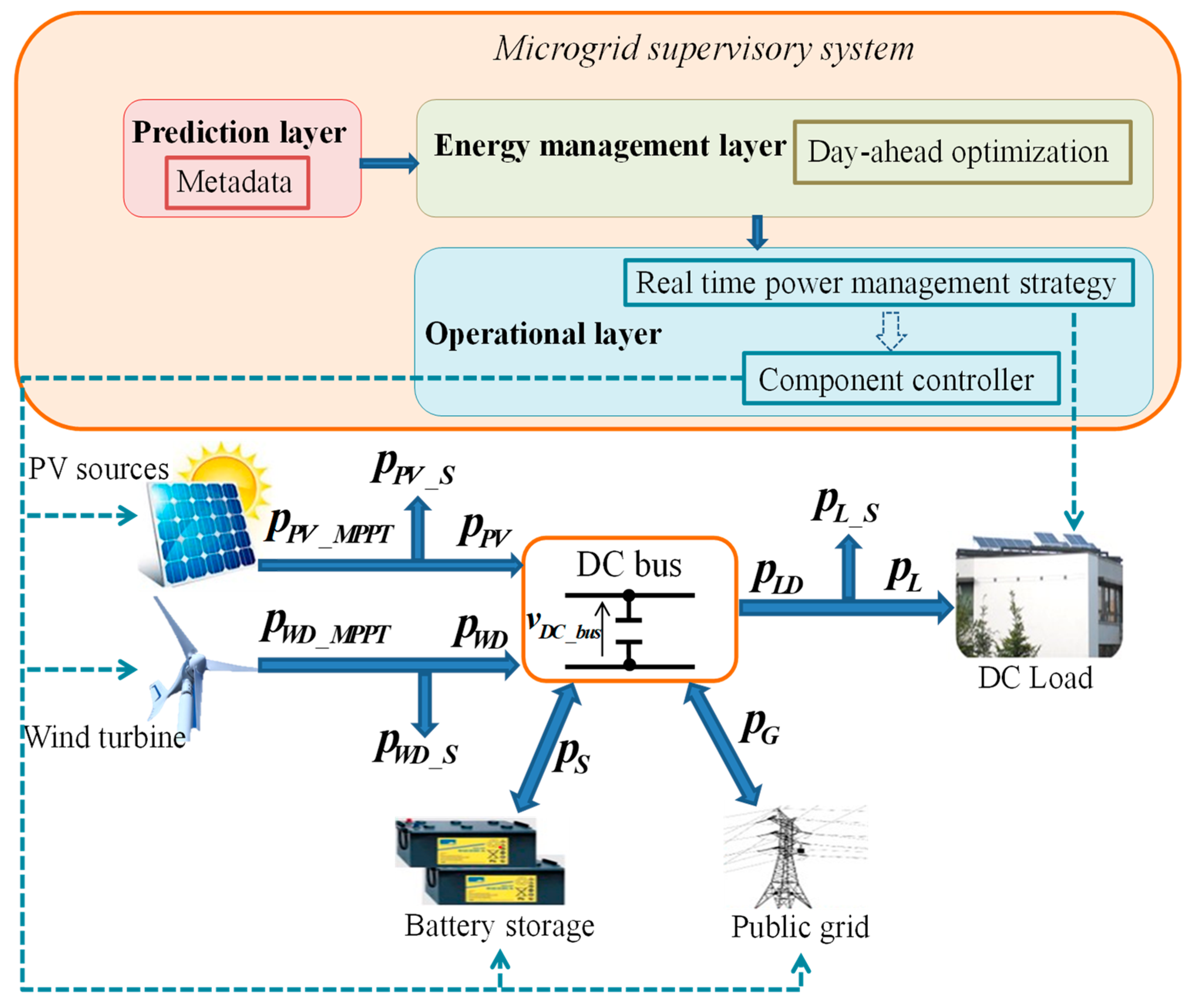
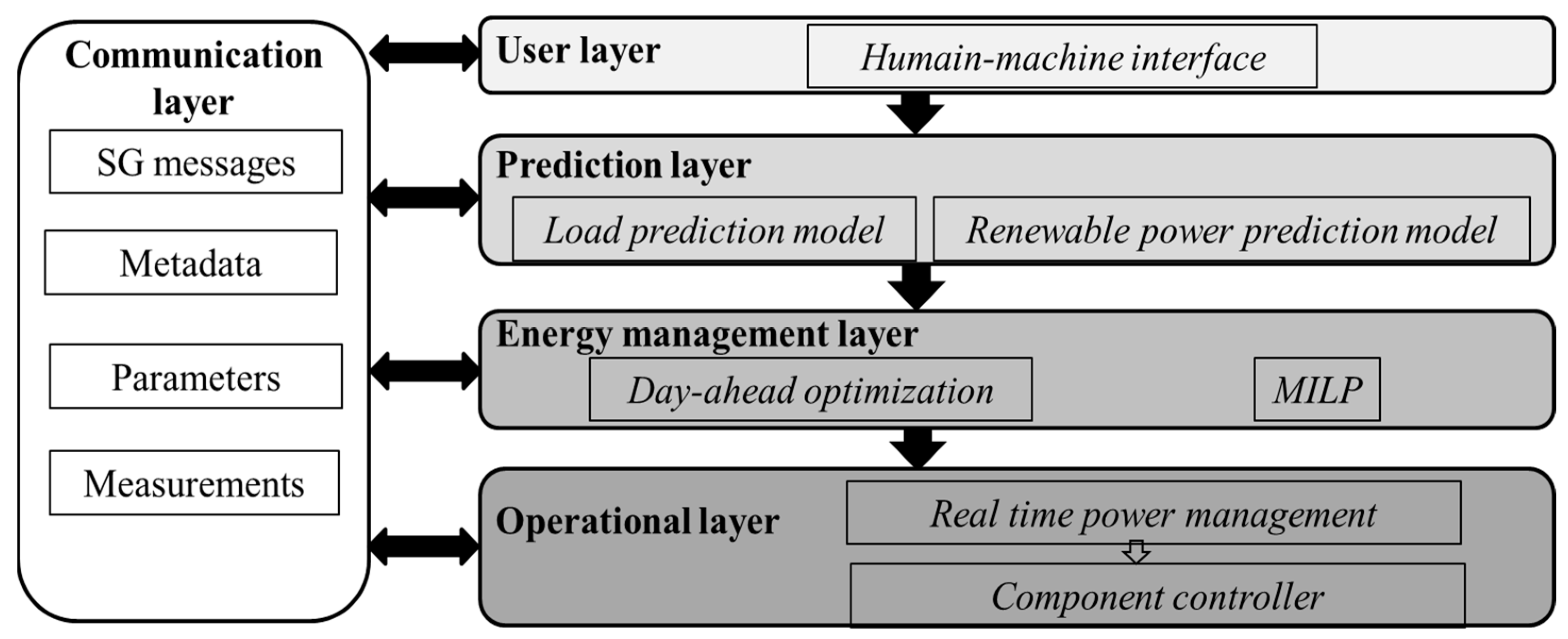
4. MG Supervision Overview

The proposed multi-layer supervisory system (Figure 2) [23] is structured into four main layers that interact among themselves and operate in at different scale times. The aim of the MG supervisory is to interact with the smart grid (SG) and the end-user. It is able to receive metadata from external sources, and keep the instantaneous power balance in the MG. Several works carried out in the Avenues unit research have been based on this structure [24,25]. Parameters refer to a group of parameters related to the MG and their physical limitations. The metadata receives the forecast data. The SG is responsible for exchanging messages and communication with the public grid. Characteristics of each layer have been explained in detail in [20].

4.1. Energy Management

The energy management layer aims to optimize and minimize the total energy cost by dispatching power flow according to the power prediction, SG messages, and measurement data under the constraints of the modeling. In this section, optimization for a grid-connected mode is studied.

Mixed-integer linear programming was chosen as a solver for the formulated problem, and the optimization was performed day-ahead by using prediction data. The optimization results were the power flows of sources and load translated into a distribution coefficient. This latter is regarded as a predictive control variable responsible for communication with the operational layer to ensure an optimal operation.

The proposed problem formulation was based on the components characteristics and constraints already presented in Equations (2)–(12). The stability of the DC bus voltage was then ensured by the power balance constraint presented in Equation (13). The controller dynamic considered for the MG was not used in this study.

$$p_{PV}(t)+p_{WD}(t)-p_L(t)=p_S(t)+p_G(t)$$

(13)

The total energy cost result of the optimization is expressed in Equation (14):

$$C_{TOTAL}=C_{PV\_S}+C_{WD\_S}+C_{L\_S}+C_S+C_G$$

(14)

where $C_{PV\_S}$ is the PV shedding energy cost, $C_{WD\_S}$ is the SSWD shedding energy cost, $C_{L\_S}$ is the load shedding energy cost, and $Cs$ is the storage energy cost, $C_G$ is the public grid energy cost.

The tariffs $C_{PV\_S}$ and $C_{WD\_S}$ are calculated in Equations (15) and (16) according to the amount of PV and SSWD shedding power.

$$C_{PV\_S}=\frac{1}{3.6\times {10}^6}{\displaystyle \sum _{t_i=t_0}^{t_F}{c}_{PVS}\left(t_i\right)\cdot \Delta t\cdot p_{PV\_S}\left(t_i\right)}$$

(15)

$$C_{WD\_S}=\frac{1}{3.6\times {10}^6}{\displaystyle \sum _{t_i=t_0}^{t_F}{c}_{WDS}\left(t_i\right)\cdot \Delta t\cdot p_{WD\_S}\left(t_i\right)}$$

(16)

The cost of load shedding is defined in Equation (17), and it introduces inconvenience for end-users:

$$C_{LS}=\frac{1}{3.6\times {10}^6}{\displaystyle \sum _{t_i=t_0}^{t_F}{c}_{LS}\left(t_i\right)\cdot \Delta t\cdot p_{L\_S}\left(t_i\right)}$$

(17)

The grid cost is defined in Equation (18), and it shows that the grid power could be bought or sold at the same price.

$$C_G=\frac{1}{3.6\times {10}^6}{\displaystyle \sum _{t_i=t_0}^{t_F}{c}_G\left(t_i\right)\cdot \Delta t\cdot (-p_{G\_I}\left(t_i\right)}+-p_{G\_S}\left(t_i\right))$$

(18)

where $p_{G\_I}$ and $p_{G\_S}$ are, respectively, the power grid and supply.

This study took into consideration a single rate for energy purchased or sold and the grid energy tariff was defined according to peak hour ($c_{PH}$) or normal hour ($c_{NH}$).

The storage cost is provided in Equation (19), and it is based on storage aging:

$$C_S=\frac{1}{3.6\times {10}^6}{\displaystyle \sum _{t_i=t_0}^{t_F}{c}_S\left(t_i\right)\cdot \Delta t\cdot (p_{S\_C}\left(t_i\right)}+p_{S\_D}\left(t_i\right))$$

(19)

where $p_{S\_C}$ and $p_{S\_D}$ are, respectively, the storage power charge and discharge.

The optimization under constraints were formulated as follow:

Minimize:

$$C_{TOTAL}=C_{PV\_S}+C_{WD\_S}+C_{L\_S}+C_S+C_G$$

(20)

with respect to:

$$\{\begin{array}{l}{p}_{PV}(t_i)+p_{WD}(t_i)+p_{S\_D}(t_i)+p_{G\_S}(t_i)=p_L(t_i)+p_{S\_C}(t_i)+p_{G\_I}(t_i)\\ p_S(t_i)=p_{S\_C}(t_i)+p_{S\_D}(t_i)\\ p_{PV}=p_{PV\_MPPT}-p_{PV\_S}\\ p_{WD}=p_{WD\_MPPT}-p_{WD\_S}\\ p_L=p_{LD}-p_{L\_S}\\ if p_{PV\_MPPT}(t_i)+p_{WD\_MPPT}(t_i)>p_{LD} then p_{L\_S}(t_i)=0\\ if p_{PV\_MPPT}(t_i)+p_{WD\_MPPT}(t_i)=0 then \{\begin{array}{l} p_{L\_S}(t_i)=0\\ p_{PV\_S}(t_i)=0\\ p_{WD\_S}(t_i)=0\end{array}\\ \\ if p_{PV\_MPPT}(t_i)+p_{WD\_MPPT}(t_i)<0 then \{\begin{array}{l} p_{PV\_S}(t_i)=0\\ p_{WD\_S}(t_i)=0\end{array}\\ SO{C}_{MIN}\le soc(t_i)\le SO{C}_{MAX}\\ soc(t_i)=so{c}_0+\frac{100\%}{3600C_{REF}{v}_S}{\displaystyle {\int }_{t_0}^{t_f}{p}_S(t_i)}dt\\ SOC(t_f)>SO{C}_f\\ p_{PV}(t_i)\ge 0\\ p_{WD}(t_i)\ge 0\\ p_L(t_i)\ge 0\\ p_{PV\_S}(t_i)\ge 0\\ p_{WD\_S}(t_i)\ge 0\\ p_{L\_S}(t_i)\ge 0\\ -P_{S\_MAX}\le p_S(t)\le P_{S\_MAX} \\ 0\le p_{G\_I}(t)\le P_{GI\_MAX}\\ 0\le p_{G\_S}(t)\le P_{GS\_MAX} \\ t_i=\left\{t_0,t_0+\Delta t,t_0+2\Delta t,\dots ,t_F\right\}\end{array}$$

(21)

All these constraints have been explained in Section 3. The three constraints preceded by “if” show that no load shedding power is allowed when the load can be fully supplied, while no PV and SSWD shedding power can occur when the PV and SSWD power can be fully consumed. Moreover, neither load shedding nor RESs power shedding can happen when there is no production from PV and SSWD.

Additional constraints showing that the storage and the grid cannot directly exchange power are given in Equation (22):

$$\{\begin{array}{l}if p_{PV\_MPPT}(t_i)+p_{WD\_MPPT}(t_i)\ge p_{LD}(t_i) then\{\begin{array}{l}{p}_G(t_i)\ge 0\\ p_S(t_i)\ge 0\end{array} \\ if p_{PV\_MPPT}(t_i)+p_{WD\_MPPT}(t_i)<p_{LD} (t_i) \mathrm{and} then \{\begin{array}{l}{p}_G(t_i)<0\\ p_S(t_i)<0\end{array}\end{array}$$

(22)

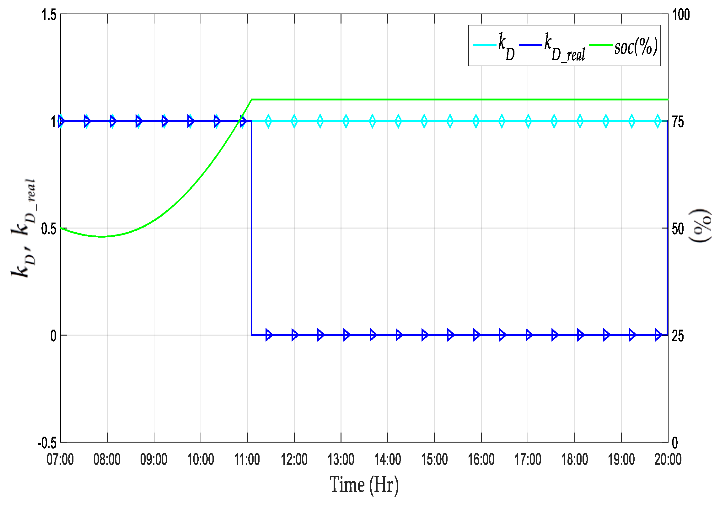
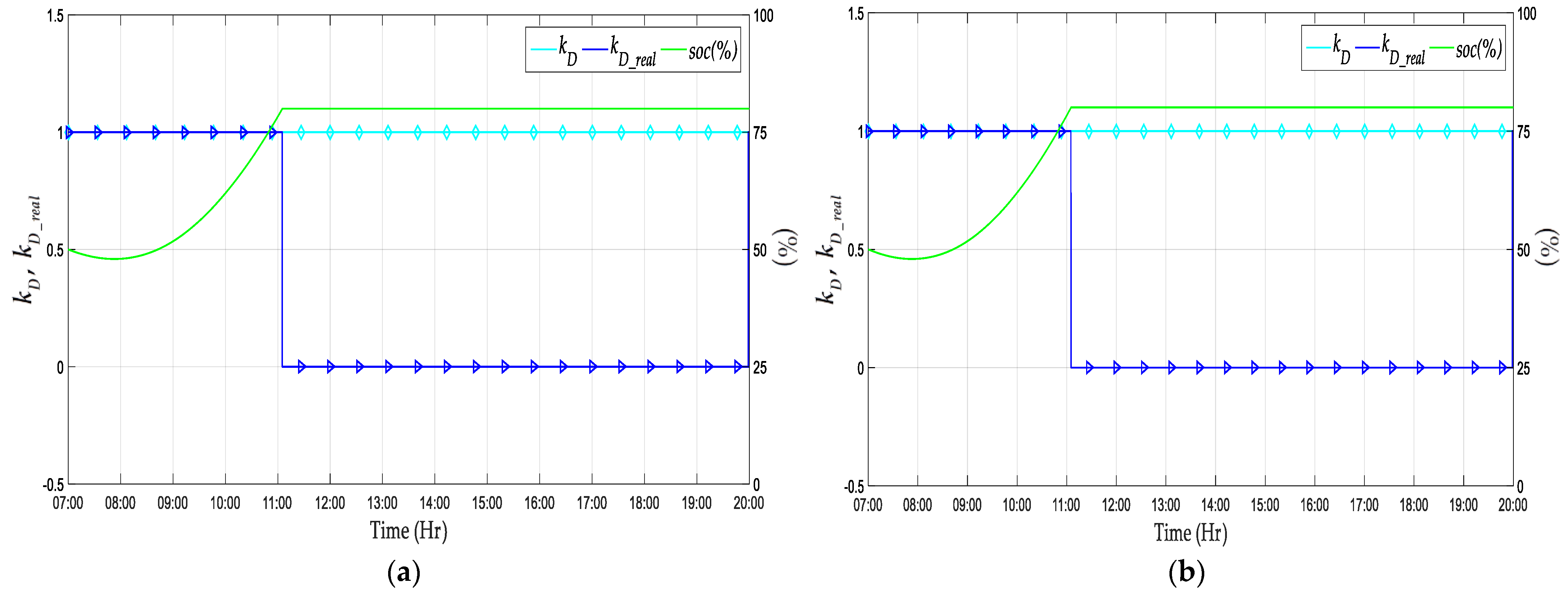
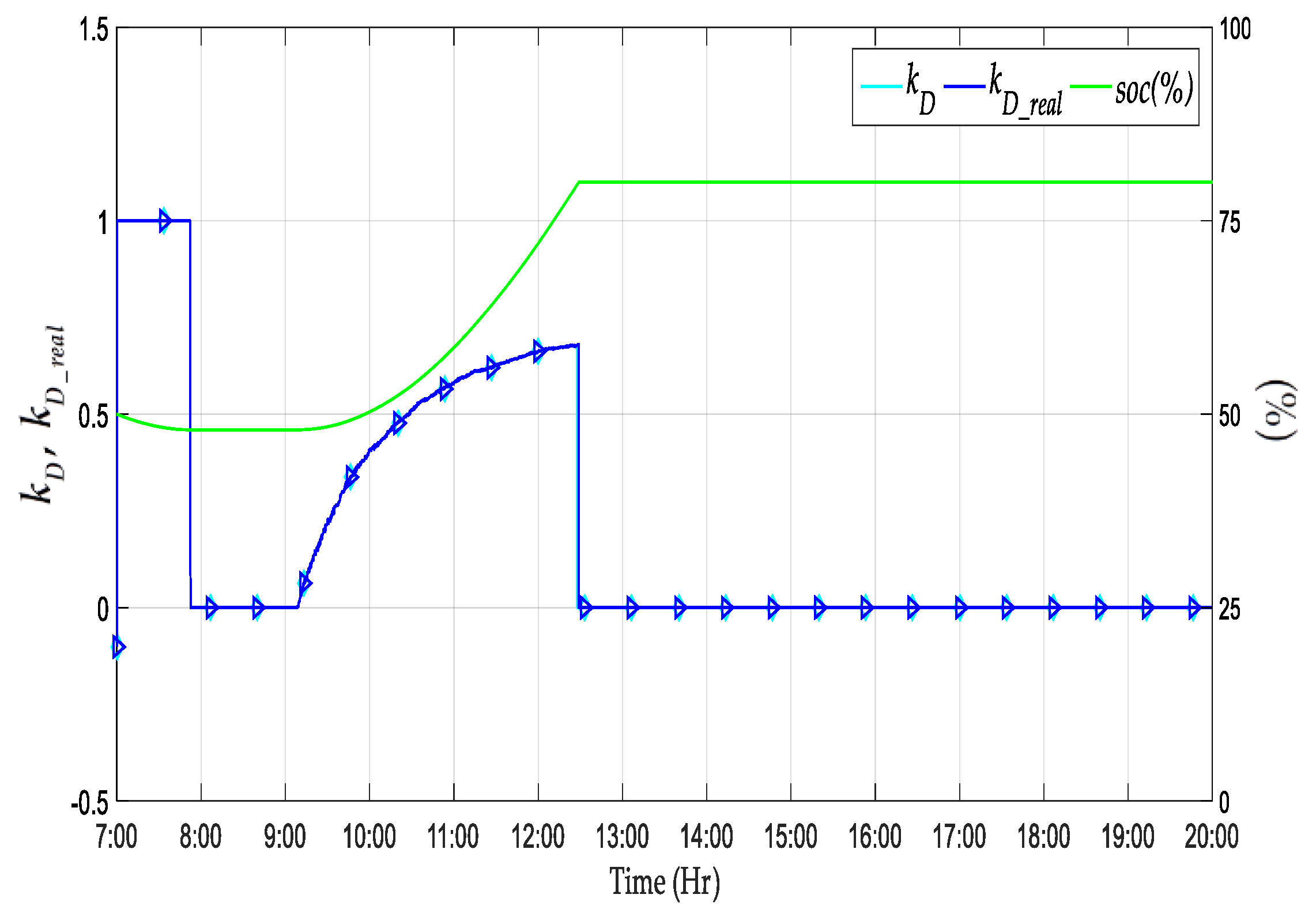
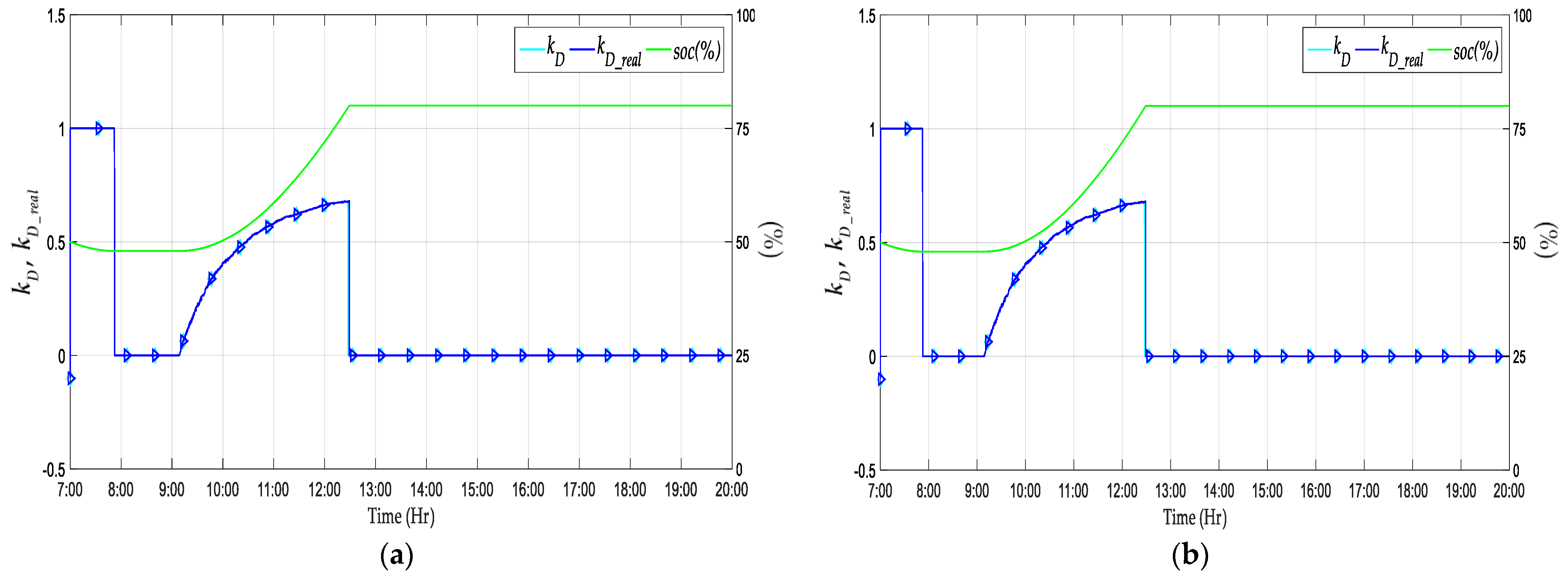
The coefficient $k_D$ is given to introduce the day-ahead optimization results into the power management layer and to decouple the system operation between the power management layer and the energy management layer. It was calculated according to (23):

$$k_D=\frac{p_S}{p_S+p_G},k_D\in \left[0,\hspace{0.17em}1\right]$$

(23)

where $k_D$ is the power distribution rate between storage and public grid.

4.2. Power Management

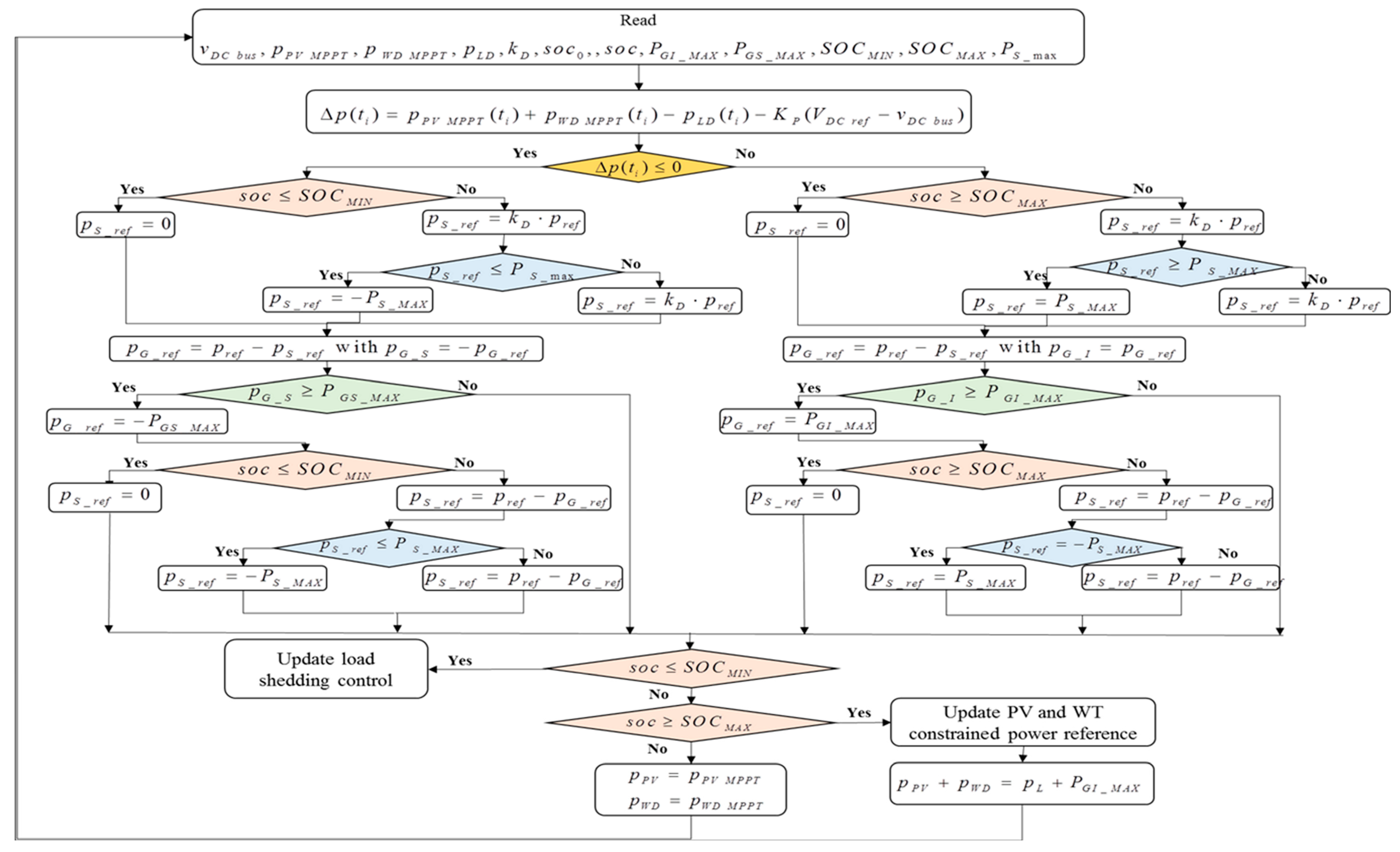
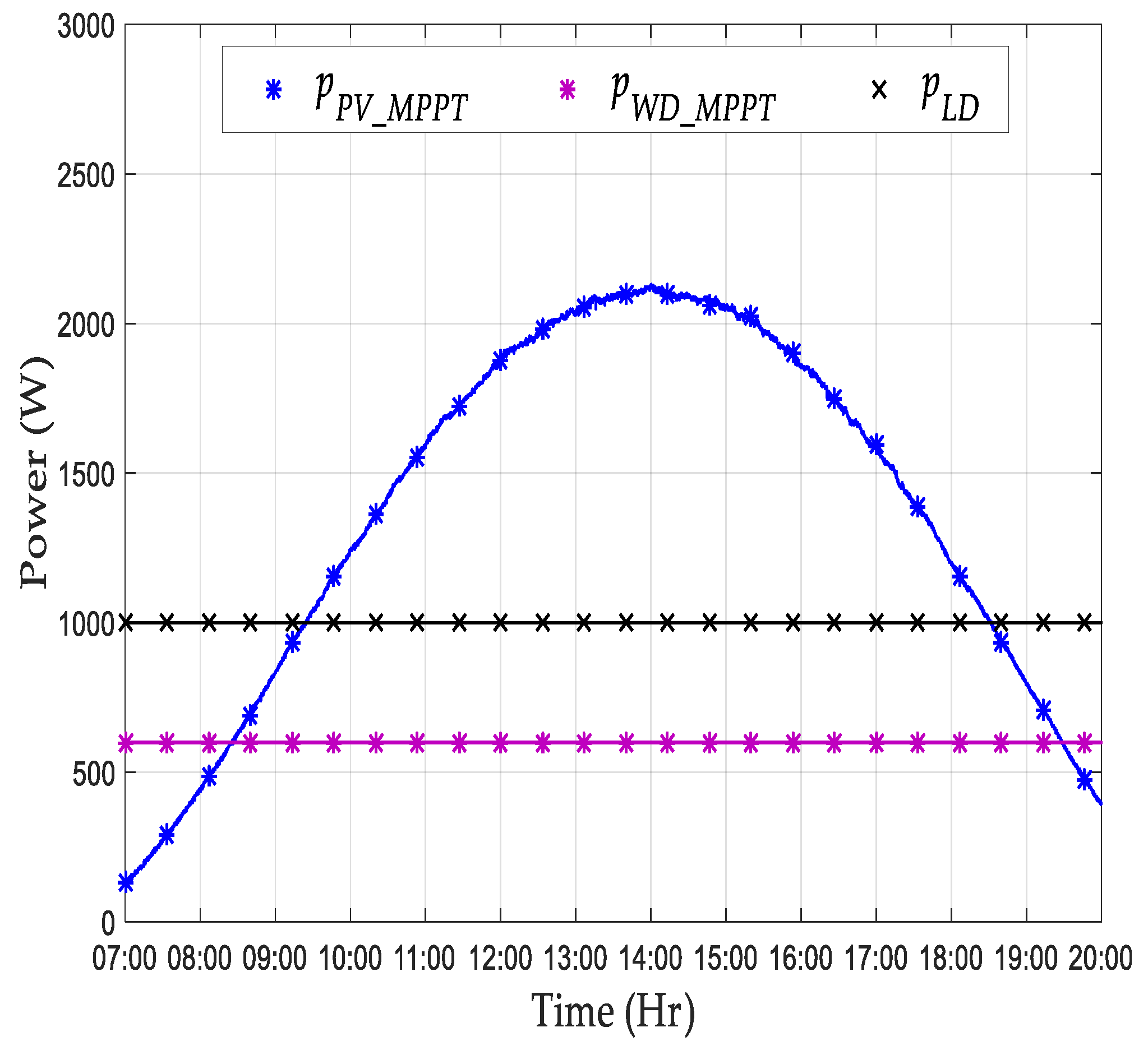
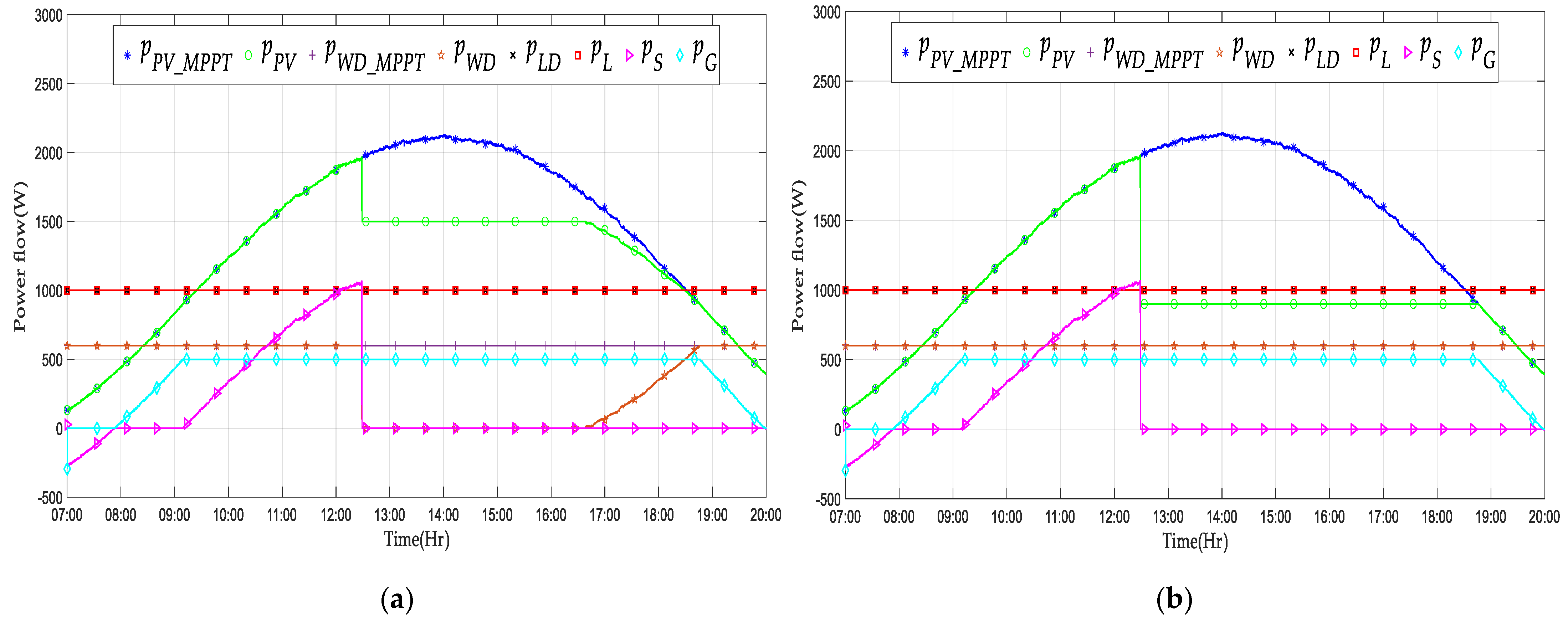
The power management is performed in the operational layer that is responsible for keeping the instant power balance and ensuring the DC bus voltage stabilization concerning the system’s constraints and physical limits. The applied algorithm started first by reading the fixed parameters, the real measurements, and the updated parameter value provided from the optimization. Second, the compensation power was calculated according to Equation (1). Using the resulting power and the distribution parameter, the power that should be exchanged with the public grid and the storage was calculated to ensure power balance and voltage stability. The suggested power management strategy is a rule-based method is presented in the flow chart given in Figure 3.

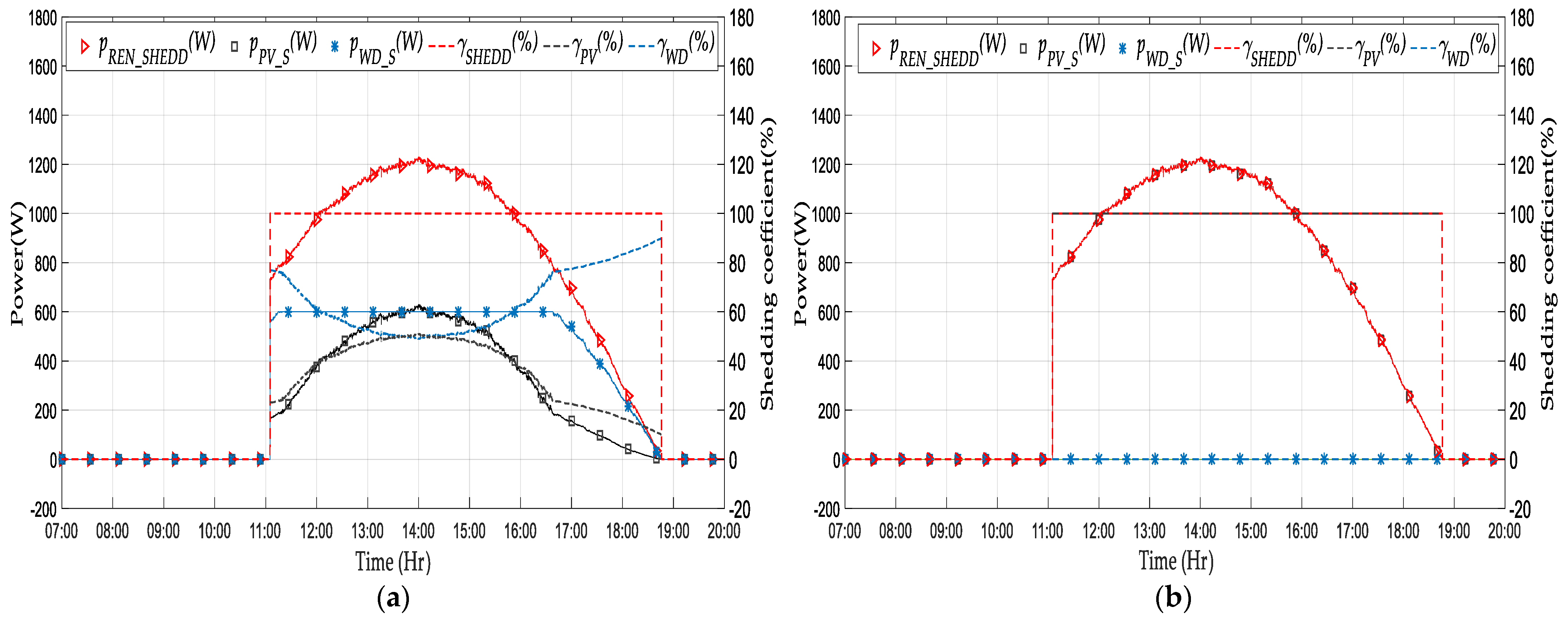
The $k_D$ is calculated in the energy management and introduced in the real-time power management strategy. As illustrated in the flow chart, the storage reference is updated two times: the first one is for power balancing before that the grid reaches its limits. Once this latter occurs a second update of the storage reference happens to perform load shedding or PV and SSWD constrained production.

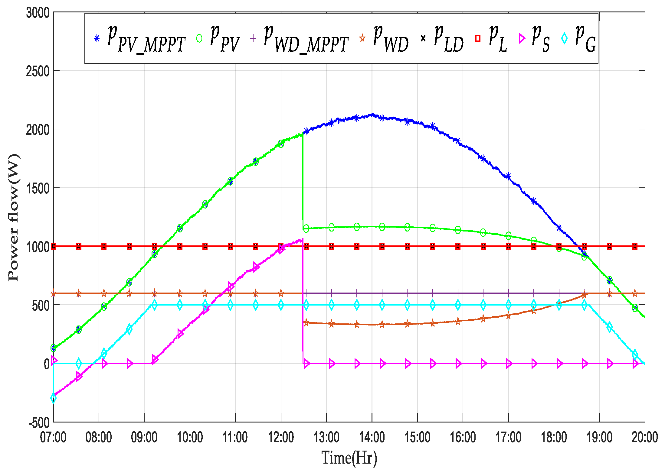
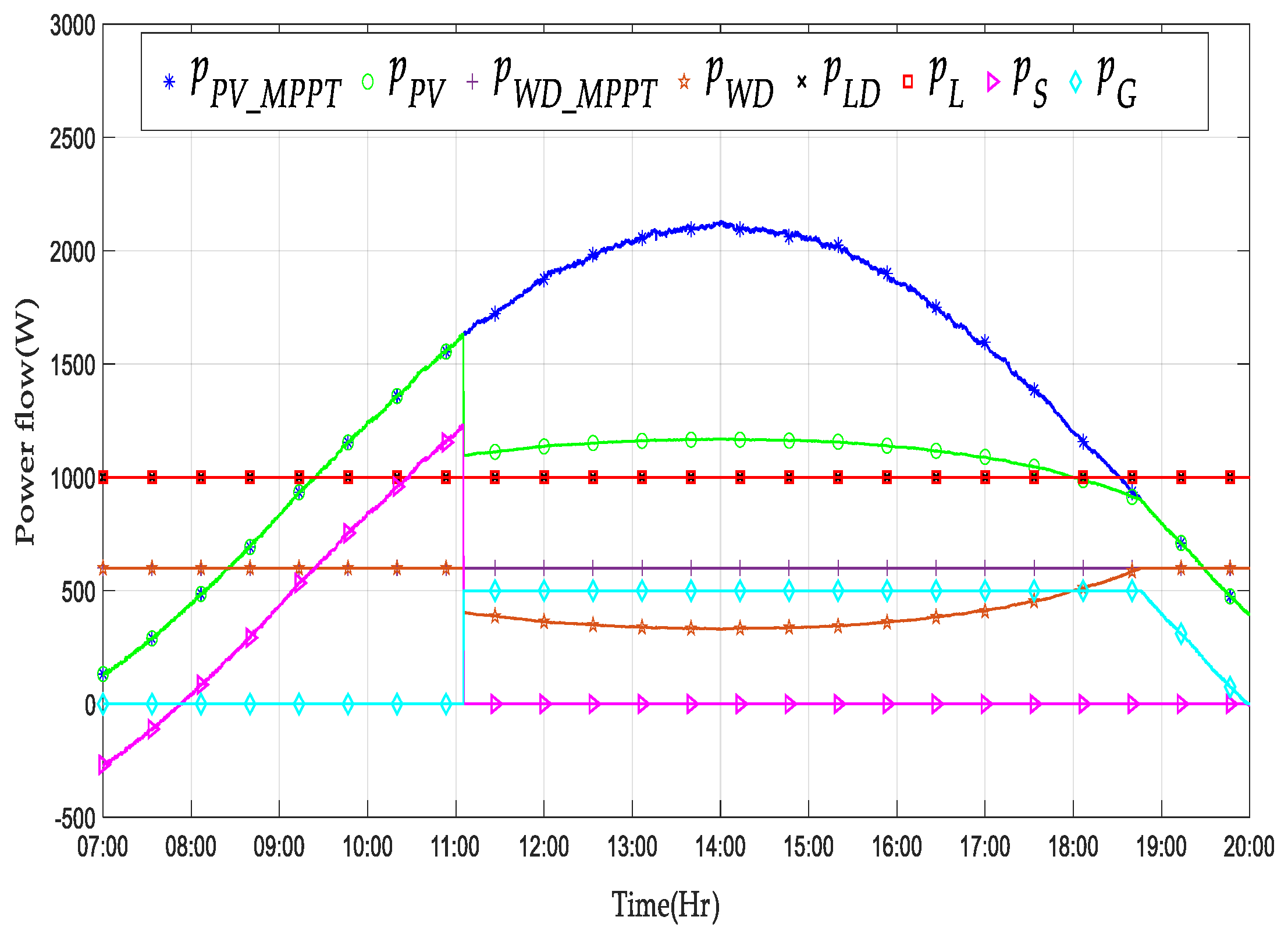
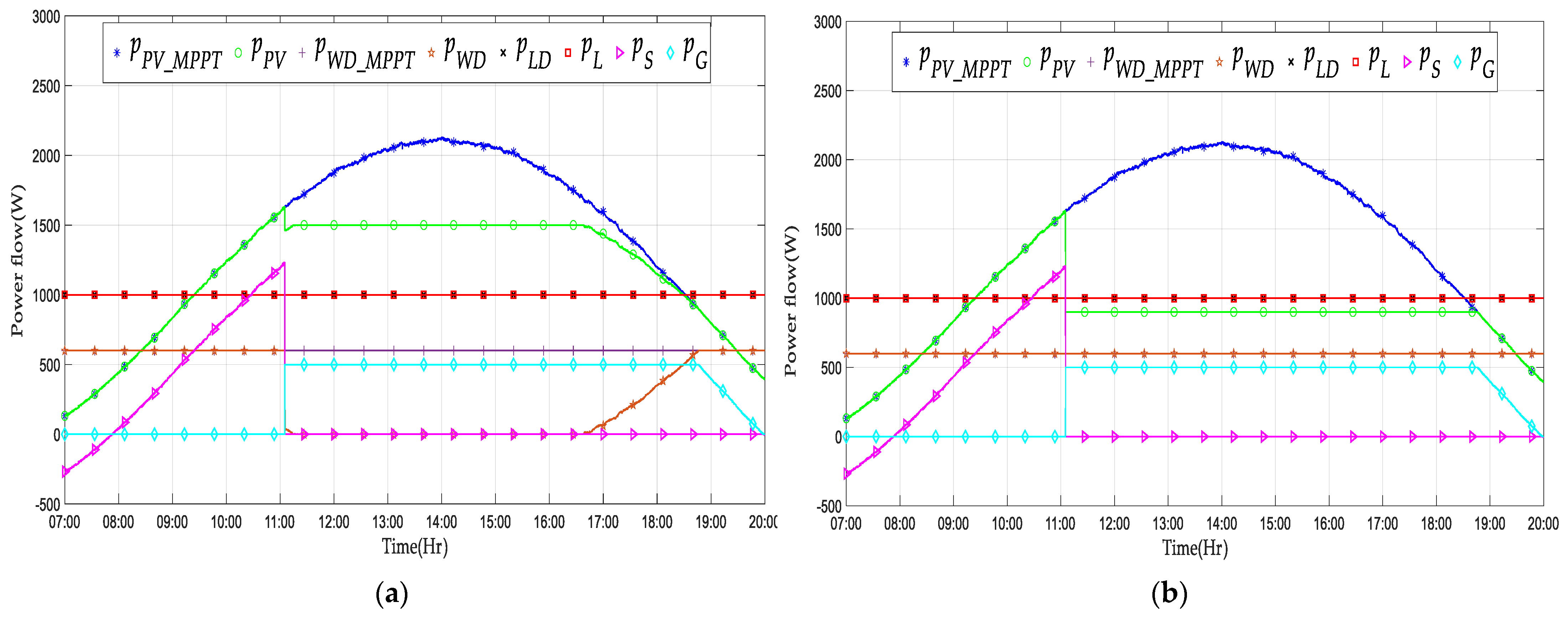
Furthermore, the proposed power management strategy consists of two extreme cases: (i) if there is a shortage of energy for supplying the load, which means that when PV panels and SSWD produce insufficient power, the grid reaches its limit, and the storage is empty. It this case, load shedding happens; (ii) if the PV panels and SSWD power production cannot be totally consumed, which means that the grid reaches its injection limit, the storage achieves the $soc$ upper limit, and the load is fully supplied or cannot consume enough, the PV and SSWD energy should be limited.

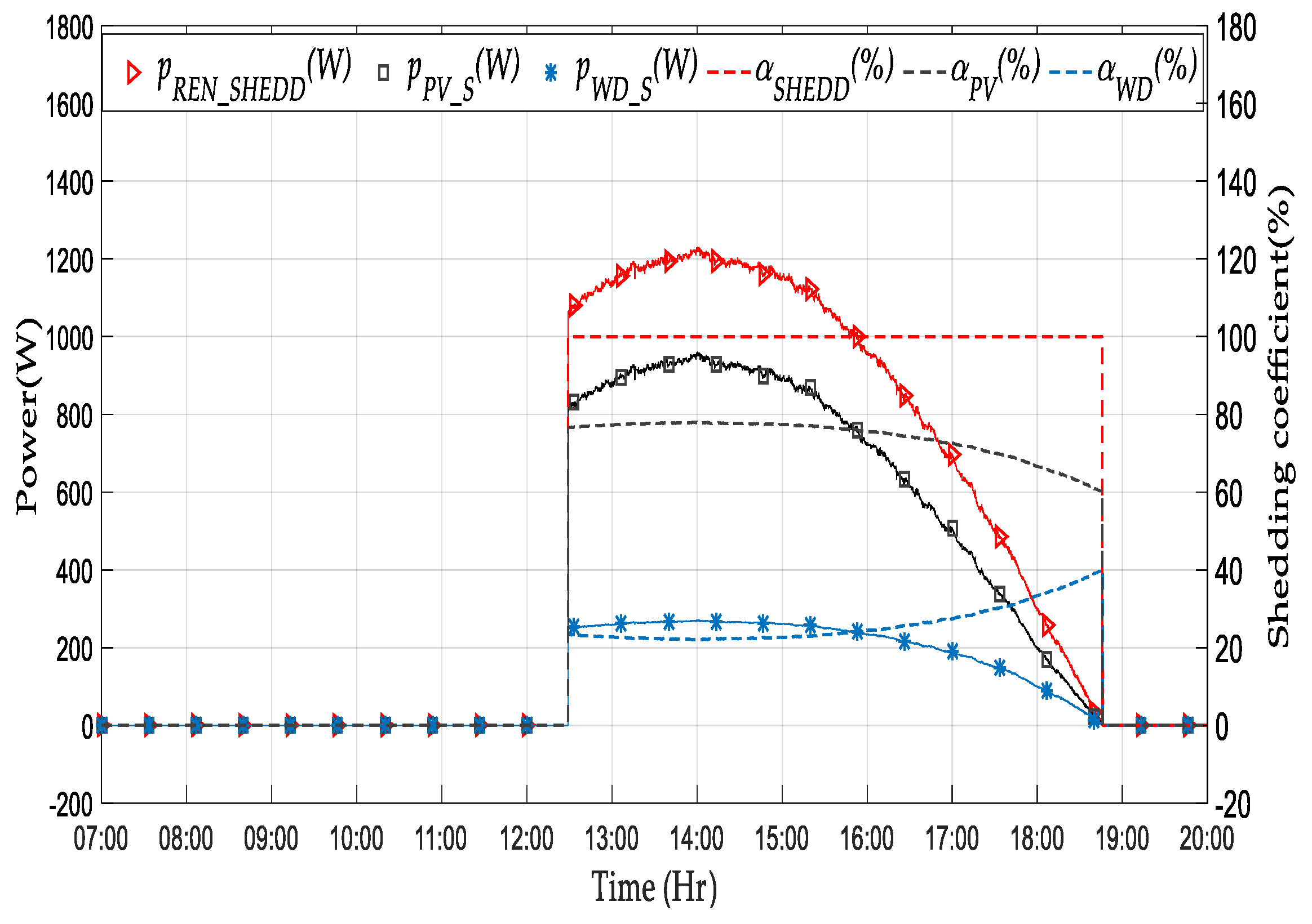
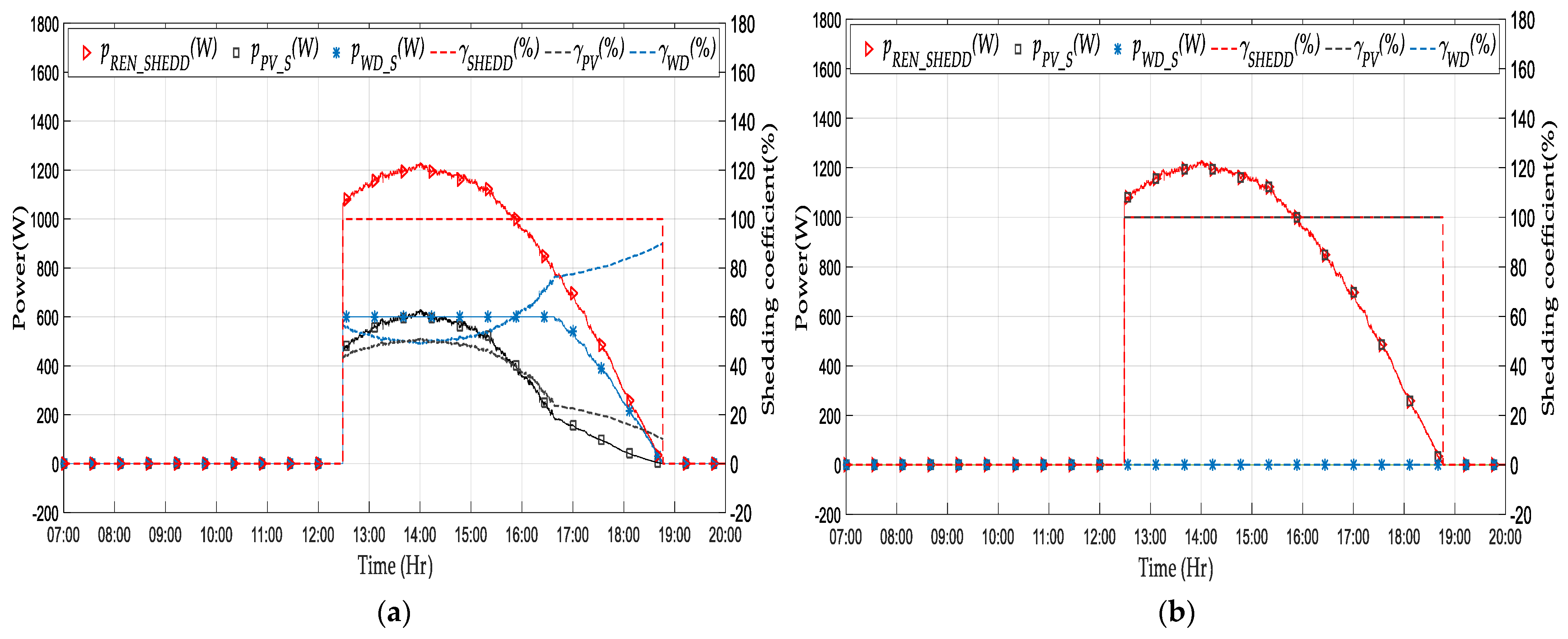
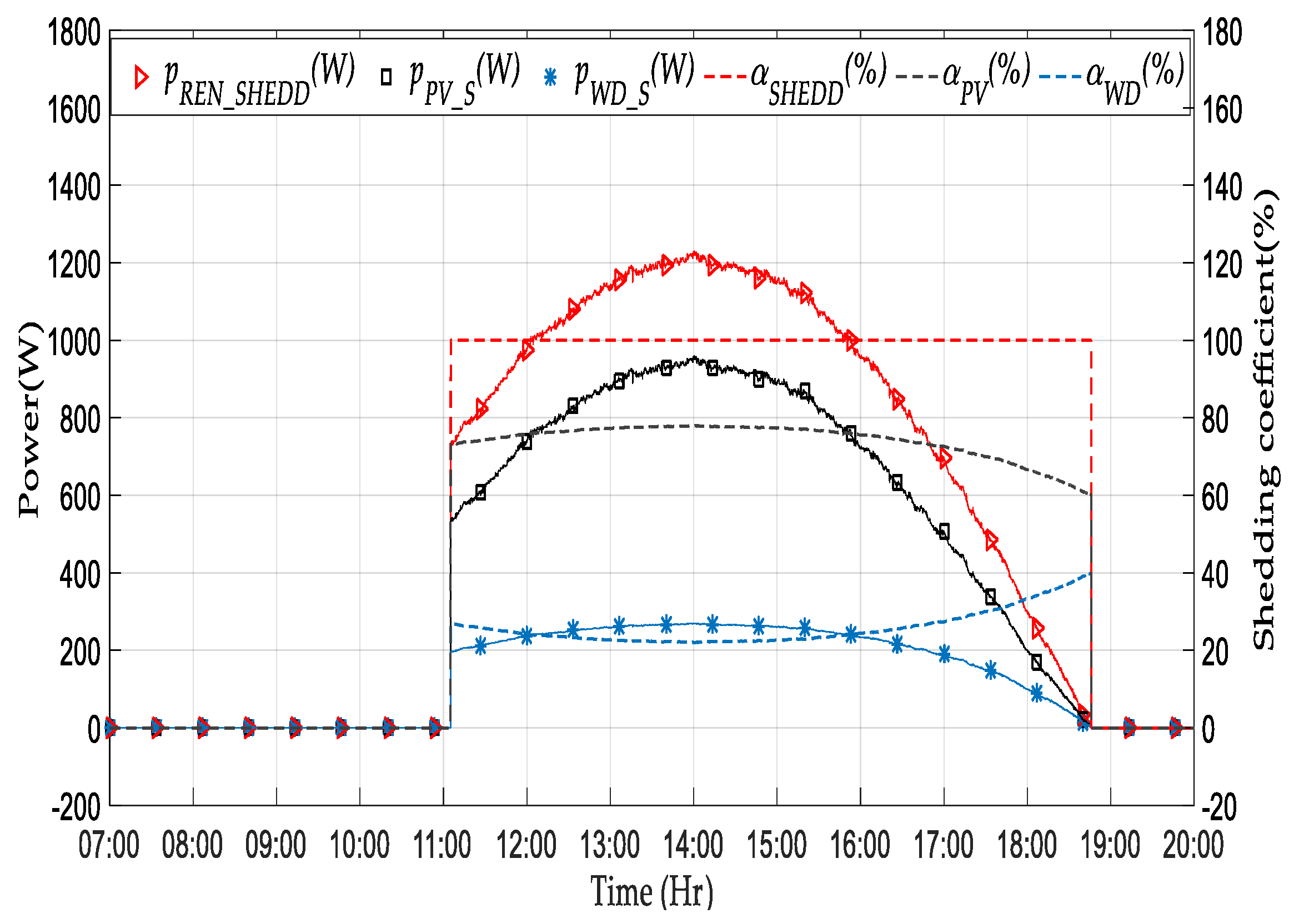
To separate and calculate the power which must be limited from each source, two coefficients called “shedding coefficients” have been proposed. The idea is to first calculate the total power, which must be shed from the two sources, and multiply it respectively by the shedding coefficients in order to define the power, which must be shed by each source.

5. Shedding Coefficients

After installation of PV sources and the SSWD, only the maintenance involves costs while the production does not need extra fees. However, shedding PV and SSWD power mean that the assets are not fully utilized. So the PV sources and SSWD power shedding are penalized in the optimization and their energy costs are already defined in Equations (15) and (16).

The total renewable power to be shed is defined as follows:

$$p_{REN\_SHEDD}=p_{PV\_S}+p_{WD\_S}=p_{PV\_MPPT}+p_{WD\_MPPT}-(p_{LD}+p_S+p_G)$$

(24)

The role of the shedding coefficients related to the RESs was not emphasized or even noticed in the case where the renewable production was completely consumed. In this case, the two renewable sources (PV sources and the SSWD) were considered as one renewable source and their production was mainly destined to feed the load and the rest to be stored in batteries or injected into the public grid (depending on the adopted power management strategy). Once the production of these RESs exceeds the needs of the MG, namely the limit of injection into the grid, limits of storage, and the load that is fully supplied, the power generation from PV sources and the SSWD must be limited. The shedding coefficients embody the principle of separation of the two sources and the calculation of the power that must be limited from each source by taking into account different criteria such as the share of each source in this excess generation and the shedding cost attributed to each source.

5.1. Alpha Coefficients

Alpha coefficients are proposed in order to calculate $p_{PV\_S}$ and $p_{WD\_S}$. They are based on the contribution of each renewable source in generating $p_{REN\_SHEDD}$ without taking into account the PV sources and the SSWD shedding costs. Thus, the source that generates more and is responsible for the excess of power should be limited more. Here, the penalization cost associated with each source is not considered. Their expressions showed the percentage of the contribution of each source in generating the total power that should be shed and they are calculated as follows:

$${\alpha }_{PV}=\frac{p_{PV\_MPPT}}{p_{PV\_MPPT}+p_{WD\_MPPT}},{\alpha }_{WD}\in \left[0,\hspace{0.17em}1\right]$$

(25)

$${\alpha }_{WD}=\frac{p_{WD\_MPPT}}{p_{PV\_MPPT}+p_{WD\_MPPT}},{\alpha }_{WD}\in \left[0,\hspace{0.17em}1\right]$$

(26)

$${\alpha }_{PV}+{\alpha }_{WD}=1$$

(27)

The PV and SSWD shed powers are then given in Equations (28) and (29), respectively:

$$p_{PV\_S}={\alpha }_{PV}.p_{REN\_SHEDD}$$

(28)

$$p_{WD\_S}={\alpha }_{WD}.p_{REN\_SHEDD}$$

(29)

5.2. Gamma Coefficients

Gamma coefficients are proposed in order to calculate $p_{PV\_S}$ and $p_{WD\_S}$. They are based not only on the contribution of each RESs in generating $p_{REN\_SHEDD}$ but also on the PV sources and the SSWD shedding costs. In fact, the percentage already calculated based on the coefficient $\alpha$ is added to another coefficient noted $\xi$. This latter reflects the impact of the shedding cost of each RESs on the global contribution of each source in generating the total power that should be shed. They are calculated as follows:

$${\gamma }_{PV}={\alpha }_{PV}+{\xi }_{PV}=\frac{p_{PV\_MPPT}}{p_{PV\_MPPT}+p_{WD\_MPPT}}+\frac{c_{WD\_S}-c_{PV\_S}}{\max (c_{PV\_S},c_{WD\_S})}$$

(30)

$${\gamma }_{WD}={\alpha }_{WD}+{\xi }_{WD}=\frac{p_{WD\_MPPT}}{p_{PV\_MPPT}+p_{WD\_MPPT}}+\frac{c_{PV\_S}-c_{WD\_S}}{\max (c_{PV\_S},c_{WD\_S})}$$

(31)

$${\gamma }_{PV}+{\gamma }_{WD}=1$$

(32)

where ${\xi }_{PV}=\frac{c_{WD\_S}-c_{PV\_S}}{\max (c_{PV\_S},c_{WD\_S})}$ and ${\xi }_{WD}=\frac{c_{PV\_S}-c_{WD\_S}}{\max (c_{PV\_S},c_{WD\_S})}$ are two coefficients that take into account the costs of shedding PV and SSWD powers, respectively.

6. Simulation Results and Analysis

6.1. Power Profile

In order to study the shedding coefficients, arbitrary power curves were selected (Figure 4). As can be seen, the maximum power provided by the WT was limited and fixed to 600 W, which was the maximal limit of the studied SSWD. The load power curve was fixed at 1000 W. The PV power curve was calculated according to the weather data recorded on the 29 June 2019 in Compiegne. In addition, the selected simulation time horizon was from 07:00 until 20:00. During this period, the DC MG operated only in on-grid mode.

The choice of such power profiles was to analyze the optimization of the DC MG in the case of production excess. In the opposite case, PV sources and the SSWD were considered as a single source of renewable energy since the amount of power that they produced was completely consumed.

6.2. Simulation Parameters

Table 1. Parameters for simulation tests.

	Parameters		Values
Grid	$P_{GI\_MAX}=P_{G\_MAX}$		500 W
	$P_{GS\_MAX}=-P_{G\_MAX}$		−500 W
Storage	$P_{S\_MAX}$		1300 W
	$SO{C}_{MIN}$		20%
	$SO{C}_{MAX}$		80%
	$so{c}_0$		50%
	$C_{REF}$		130 Ah
	$v_s$		48 V (4 × 12)
DC bus	$V_{DC ref}$		400 V
PV sources	$N_{PV}$		18
	$P_{PV\_STC}$		25 W
SSWD	$P_{WD\_MPPT}$		600 W
DC load	$P_{LD}$		1000 W
Tariffs	$c_G$	$c_{NH}$	0.1 €/kWh
		$c_{PH}$(11:00–13:00 and 18:00 20:00)	0.7 €/kWh
	$c_S$		0.01 €/kWh
	$c_{PVS}$		1 or 2 €/kWh
	$c_{WDS}$		1 or 2 €/kWh
	$c_{LS}$		1.8 €/kWh

shows the parameters values, which were tested during the simulation. The grid tariff proposed in normal hour $c_{NH}$ was close to the ones proposed by most energy providers, while for peak hours, $c_{PH}$, a penalized purchase tariff was chosen to perform power peak shaving. Other tariffs were chosen arbitrarily, but they respected the logic of management strategy, which is an energy trend for the next 20 years. Thus, the energy tariffs were considered in the order given by Equation (33):

$$c_{PVS,WDS,LS}\gg c_{PH}>c_{NH}>c_S$$

(33)

6.3. Simulation Results and Analysis

The DC MG supervisory control for grid-connected mode was simulated based on the power profile presented in Figure 4. The system was put into a situation of energy excess produced by renewable sources and the power flow in two instances, depending on the value of $k_D$, was analyzed. The first instance was based on a constant value of $k_D$ which was equal to 1. In this case, the simulation was carried out without optimization, and the power balanced was ensured by the storage first and the grid intervened only when the storage had reached its limits. This is called “storage priority”. The second instance was about a power flow simulation controlled by a variable $k_D$ provided from the optimization calculation under CPLEX. This case is called “optimization”. Shedding coefficients mentioned in Section 5 were applied for these two power management strategies. The power management of the DC MG was verified in MATLAB/Simulink, and the optimization was performed using CPLEX [22].

6.3.1. Simulation Scenarios

The power balancing control in the operational layer was an independent function that can work with any value of $k_D(t)$. Thus, the two scenarios’ cases presented in

Table 2. Simulation cases.

Cases	α Coefficient	γ Coefficient
Storage priority ($k_D=1$)	YES	YES
Optimization ($k_D=k_D(t)$)	YES	YES

were applied to show the influence of shedding coefficients on the operation cost of the DC MG.

6.3.2. Simulation without Optimization (Storage Priority)

6.3.2.1. Power Flow Controlled by the Coefficient $\alpha$ for $c_{PVS}>c_{WDS}$ and $c_{PVS}<c_{WDS}$ in the Case of Priority Storage

The power management strategy mentioned in the flowchart of Figure 3 was implemented using the MATLAB/Simulink environment. $k_D$ (cyan bleu curve) and $k_{D\_real}$ (blue curve) represent the same variable. In fact, $k_D=1$ was selected to show that the storage had a higher priority than the public grid to supply the DC MG while $k_{D\_real}$ represented the real value of $k_D$ during the simulation depending on the use or not of the storage.

First, in Figure 5, the $k_D$ was set to 1 during the period of 07:00–11:05, meaning that only the storage was used. In the period 07:00–08:00, the $soc$ decreased first which indicated that the storage was discharging. After that, in the period 08:10–11:05, the storage started recharging, which is explained by the increase in the $soc$. At 11:05, $k_D$ should switched to 0 ($k_{D\_real}$) and $soc$ stabilize at the upper limit (80%). It is crucial to mention that the evolution of $k_D$ is the same whatever the value of PV or SSWD shedding tariff.

Regarding the power flow provided in Figure 6, the period 07:00–07:55 was characterized by supplying DC load (red line) using the total power produced by PV sources (blue line) and the SSWD (purple line) and also discharging the storage (magenta curve). From 07:55 until 11:05, the power produced by renewable sources was enough to supply the DC load and contribute to charging the storage. At 11:05, the storage was full, and turned into 0, allowing the public grid (cyan bleu curve) to ensure the power balance. After at 11:05, the load was fully fed, the storage was completely charged, and the grid reached its limit of injection, the PV and SSWD shedding happened. The blue and purple curves are, respectively, the $p_{PV\_MPPT}$ and $p_{WD\_MPPT}$ that are usually provided to meet the power balance and should be limited. The green and the brown curves show the new powers that should be provided. At 18:40, the power balance was again ensured by the public grid that was injected until 20:00.

Figure 7 presents the period where the PV and SSWD shedding occurred in the case of storage priority. As can be seen in this figure, the amount of power that each renewable source should shed was calculated using the $\alpha$ coefficient. The duration of shedding lasted for 7 h and 45 min (11:05–18:40). Therefore, in order to compare shedding powers of PV source and the SSWD (black square and blue star markers, respectively), percentages (black and blue dashes lines) were calculated depending on the total power that should be shed $p_{REN\_SHEDD}$ (red triangle marker) and the $\alpha$ coefficient. The results (

Table 3. Energy shedding calculation for the $\alpha$ coefficient in the case of storage priority.

	Storage Priority $\mathit{\alpha }$
	${\mathit{c}}_{\mathit{P}\mathit{V}\mathit{S}}>{\mathit{c}}_{\mathit{W}\mathit{D}\mathit{S}}$$(2 > 1 (€/\mathbf{kWh}\left)\right) \mathbf{or} {\mathit{c}}_{\mathit{P}\mathit{V}\mathit{S}}<{\mathit{c}}_{\mathit{W}\mathit{D}\mathit{S}} (1 < 2 (€/\mathbf{kWh}\left)\right)$
	PV	SSWD
Total energy shedding (kWh)	6.74
Energy shedding per source (kWh)	5.1	1.64
Contribution of each source (%)	75.8	24.2

) clearly show that these power percentages were identical whatever the used tariffs ($c_{PVS}>c_{WDS}$ or $c_{PVS}<c_{WDS}$). In fact, $p_{PV\_S}$ constituted around 75.8% of $p_{REN\_SHEDD}$, while $p_{WD\_S}$ was about 24.2% of this power. Thus, applying coefficient $\alpha$ provided the same distribution of power that should be shed from each source without taking into account the shedding tariffs.

6.3.2.2. Power Flow Controlled by the Coefficient $\gamma$ for $c_{PVS}>c_{WDS}$ and $c_{PVS}<c_{WDS}$ in the Case the of Priority Storage

The evolution of $k_D$, $k_{D\_real}$, and $soc$ in the simulation without optimization by applying the $\gamma$ coefficient are shown in Figure 8a,b. During the period from 07:00 to 11:05 the $k_D$ was set to 1, which indicated that only the storage was used, while $k_{D\_real}$ represents the real value of $k_D$ during the simulation depending on the use or not of the storage. In the period between 07:00 and 07:55, the $soc$ decreased, which means that the storage was discharging, while in the period from 07:55 to 11:05, the $soc$ increased until reaching the upper limit. At 11:05, $k_D$ switched to 0 ($k_{D\_real}$) and the $soc$ stabilized at 80%.

Concerning the power flow provided in Figure 9a,b, the period from 07:00 to11:05 was characterized by using the total power produced by PV sources (blue line) and the SSWD (purple line) to supply the DC load (red line) and recharge the storage (magenta curve). At 11:05, the storage was full, and turned into 0, letting the public grid (cyan bleu curve) ensure the power balance. At 11:05, the load was fully fed (1000 W), the storage was completely charged (1300 W), and the grid had reached its limit of injection (500 W). Then, the excess of power from PV and SSWD should be limited. Since $\gamma$ takes into account the shedding tariff of each source, a difference in the amount of power that should be limited from each source was then noticed. The blue and purple curves are, respectively, the $p_{PV\_MPPT}$ and the $p_{WD\_MPPT}$ that are normally provided and the green and the brown curves, ($p_{PV}$ and $p_{WD}$, respectively) show the limited powers that should be provided to meet the power balance. It can be noticed in Figure 9a ($c_{PVS}>c_{WDS}$) that the SSWD power was totally limited (the SSWD turned off) in the period from 11:05 to 16:40, while the rest of the power was limited from the PV source. However, when $c_{PVS}<c_{WDS}$(Figure 9b) and since an important amount of power was produced by PV sources, only these later were limited and the SSWD continued to produce at its maximum power. At 18:40, the power balance was again ensured by the public grid that was injected until 20:00.

Figure 10a,b present periods where the shedding occurred for PV and SSWD in the case of storage priority by applying $\gamma$ for $c_{PVS}>c_{WDS}$ and $c_{PVS}<c_{WDS}$, respectively. As can been seen in these figures, the amount of power that should be shed by each renewable source was calculated using the $\gamma$ coefficient and different shedding tariffs. Durations of shedding were identical (7 h 45 min). Nevertheless, in the case of $c_{PVS}>c_{WDS}$, both PV sources and the SSWD (black square and blue star markers, respectively) were contributing to limiting the $p_{REN\_SHEDD}$ (red triangle marker), while in the case of $c_{PVS}<c_{WDS}$, only PV sources were responsible for the power balance ($p_{REN\_SHEDD}$ and $p_{PV\_S}$ lines are combined). Thus, in order to compare shedding powers of PV sources and the SSWD, respectively, percentages (black and blue dashes lines) were calculated depending on $p_{REN\_SHEDD}$ and the $\gamma$ coefficient.

Table 4. Energy shedding calculation for the $\gamma$ coefficient in the case of storage priority.

	Storage Priority $\mathit{\gamma }$
	${\mathit{c}}_{\mathit{P}\mathit{V}\mathit{S}}>{\mathit{c}}_{\mathit{W}\mathit{D}\mathit{S}} (2 > 1 (€/\mathbf{kWh}\left)\right)$		${\mathit{c}}_{\mathit{P}\mathit{V}\mathit{S}}<{\mathit{c}}_{\mathit{W}\mathit{D}\mathit{S}} (1 < 2 (€/\mathbf{kWh}\left)\right)$
	PV	SSWD	PV	SSWD
Total energy shedding (kWh)	6.74		6.74
Energy shedding per source (kWh)	2.71	4.03	6.74	0
Contribution of each source (%)	40.2	59.8	100	0

provides these percentages according to the simulation cases. The results clearly showed that in the case of $c_{PVS}>c_{WDS}$, $p_{PV\_S}$ and $p_{WD\_S}$ constituted 40.2% and 59.8% of $p_{REN\_SHEDD}$, respectively. Otherwise, when $c_{PVS}<c_{WDS}$, only PV sources were limited (100% of $p_{REN\_SHEDD}$).

6.3.3. Simulation with Optimization

6.3.3.1. Power Flow Controlled by the Coefficient $\alpha$ for $c_{PVS}>c_{WDS}$ and $c_{PVS}<c_{WDS}$ in the Case of Optimization

The optimization issue was solved by CPLEX in the energy management layer. Indeed, this latter provided the optimum energy flow management that helped to calculate $k_D(t)$. The distribution coefficient was then transmitted to the operational layer to run the power system.

As can be observed in Figure 11, $k_D$ (cyan bleu curve) and $k_{D\_real}$ (blue curve) were confused since $k_D$ was the result of the optimization. During the period between 07:00 and 07:55, the $k_D$ was set to 1, which indicated that only the storage was used. In addition, the $soc$ decreased during this period, meaning that the storage was discharging. In the period from 09:10 to12:30, the value of $k_D$ evolved between 0 and 1, indicating that both the public grid and storage supported the MG. It can be notice that, despite the difference in the value of PV or SSWD shedding tariff, the evolution of $k_D$ still remained the same.

Concerning the power flow provided in Figure 12, the power balance in the period from 07:00 to 07:55 was ensured by discharging the storage and using the production of PV sources and the SSWD. From 07:55 to 12:30, the total power produced by PV sources (blue line) and the SSWD (purple line) was used to supply the DC load (red line), recharged the storage (magenta curve), and was injected into the public grid (cyan bleu curve). After 12:30, the load was fully fed, the storage was completely charged, and the grid reached its limit of injection, therefore, PV and SSWD shedding happened. The blue and purple curves are, respectively, the $p_{PV\_MPPT}$ and $p_{WD\_MPPT}$ that are normally provided but to meet the power balance, these powers should be limited. The new powers that should be provided are shown by the green and the brown curves. At 18:40, the power balance was again ensured by the public grid that was injected until 20:00.

Figure 13 presents the period where the PV and SSWD shedding occurred in the case of optimization. As can be seen in this figure, the amount of power that should be shed by each renewable source was calculated using the $\alpha$ coefficient. The duration of shedding lasted for 6 h and 10 min (12:30–18:40). Therefore, in order to compare shedding powers of PV source and the SSWD (black square and blue star markers, respectively), percentages (black and blue dashes lines) were calculated depending on the total power that should be shed $p_{REN\_SHEDD}$ (red triangle marker) and the $\alpha$ coefficient. The results in

Table 5. Energy shedding calculation for the $\alpha$ coefficient in the case of optimization.

	Optimization $\mathit{\alpha }$
	${\mathit{c}}_{\mathit{P}\mathit{V}\mathit{S}}>{\mathit{c}}_{\mathit{W}\mathit{D}\mathit{S}}$$(2 > 1 (€/\mathbf{kWh}\left)\right) \mathbf{or} {\mathit{c}}_{\mathit{P}\mathit{V}\mathit{S}}<{\mathit{c}}_{\mathit{W}\mathit{D}\mathit{S}}(1 < 2 (€/\mathbf{kWh}\left)\right)$
	PV	SSWD
Total energy shedding (kWh)	5.46
Energy shedding per source (kWh)	4.15	1.31
Contribution of each source (%)	76	24

were identical whatever the used tariffs ($c_{PVS}>c_{WDS}$ or $c_{PVS}<c_{WDS}$). In fact, $p_{PV\_S}$ constituted around 76% of $p_{REN\_SHEDD}$, while $p_{WD\_S}$ reached 24% of this power. Thus, applying coefficient $\alpha$ provided the same distribution of power that should be shed from each source without taking into account the shedding tariffs.

6.3.3.2. Power Flow Controlled by the Coefficient $\gamma$ for $c_{PVS}>c_{WDS}$ and $c_{PVS}<c_{WDS}$ in the Case of Optimization

Figure 14a,b show that $k_D$ and $k_{D\_real}$ were confused since $k_D$ is the result of the optimization. In the period between 07:00 and 07:55, $k_D$ was set to 1 and the $soc$ also decreased, which means that the storage was discharging, while in the period 09:10–12:30 the value of $k_D$ varied between 0 and 1, indicating that both the public grid and storage supported the MG.

Regarding the power flow provided in Figure 15a,b, the period 07:00–12:30 was first characterized by using the power produced by PV sources (blue line) and the SSWD (purple line) and discharging the storage (magenta curve) to supply the DC load (red line) (07:00–07:55) and second, by using the total renewable power to feed the DC load, recharge the storage and to be injected into the public grid (cyan bleu curve) (07:55:12:30). The PV and SSWD shedding happened at 12:30 since the load was fully fed, the storage was completely charged, and the grid had reached its limit of injection. The blue and purple curves are, respectively, the $p_{PV\_MPPT}$ and $p_{WD\_MPPT}$ that are normally provided to meet the power balance, these powers should be limited (green and the brown curves). Thus, in Figure 15a, where $c_{PVS}>c_{WDS}$, the SSWD was turned off in the period from12:30 to 16:40 and the rest of the power that should be limited was subtracted from the production of the PV sources. Nonetheless, when $c_{PVS}<c_{WDS}$ (Figure 15b) only PV sources were limited and the SSWD continued to produce at its maximum power. At 18:40, the power balance was again ensured by the public grid that was injected until 20:00.

Figure 16a,b present periods where the shedding occurred for PV sources and the SSWD in the case of optimization by applying $\gamma$ for $c_{PVS}>c_{WDS}$ and $c_{PVS}<c_{WDS}$, respectively. The durations of shedding were identical (6 h10 min) and calculated depending on the $\gamma$ coefficient and different shedding tariffs. It was noticed that in the case of $c_{PVS}>c_{WDS}$, both PV sources and SSWD (blue star marker) powers were limited. Yet, when $c_{PVS}<c_{WDS}$, $p_{REN\_SHEDD}$ (red triangle marker) and $p_{PV\_S}$ (black square marker) were combined, which means that only PV sources power was limited. Consequently, percentages (black and blue dashes lines) were calculated depending on $p_{REN\_SHEDD}$ and the $\gamma$ coefficient with the aim to compare shedding powers of PV sources and the SSWD, respectively.

Table 6. Energy shedding calculation for coefficient $\gamma$ in the case of optimization.

	Optimization $\mathit{\gamma }$
	${\mathit{c}}_{\mathit{P}\mathit{V}\mathit{S}}>{\mathit{c}}_{\mathit{W}\mathit{D}\mathit{S}}(2 > 1 (€/\mathbf{kWh}\left)\right)$		${\mathit{c}}_{\mathit{P}\mathit{V}\mathit{S}}<{\mathit{c}}_{\mathit{W}\mathit{D}\mathit{S}}(1 < 2 (€/\mathbf{kWh}\left)\right)$
	PV	SSWD	PV	SSWD
Total energy shedding (kWh)	5.46		5.46
Energy shedding per source (kWh)	2.26	3.2	5.46	0
Contribution of each source (%)	41.5	58.5	100	0

provides these percentages according to simulation cases. The results clearly showed that in the case of $c_{PVS}>c_{WDS}$, $p_{PV\_S}$ and $p_{WD\_S}$ constituted 41.5% and 58.5% of $p_{REN\_SHEDD}$, respectively. Otherwise, when $c_{PVS}<c_{WDS}$ only PV sources were limited ($p_{PV\_S}$ 100% of $p_{REN\_SHEDD}$).

6.3.4. Energy Cost Comparisons

In order to make cost comparisons of energy calculated using shedding coefficients, the case where $c_{PVS}>c_{WDS}$ was selected. The energy costs calculated by $\alpha$ and $\gamma$ coefficients are listed in

Table 7. Energy cost calculation for $\alpha$ and $\gamma$ coefficients.

Cost (€)	$\mathit{\alpha }$			$\mathit{\gamma }$
	Storage Priority	Optimization	Cost Decrease	Storage Priority	Optimization	Cost Decrease
$C_{PV\_S}$	10.21	8.3		5.41	4.54
$C_{WD\_S}$	1.63	1.31		4.03	3.20
$C_{L\_S}$	0	0		0	0
$C_G$	−1.4	−1.55		−1.4	−1.55
$C_S$	0.02	0.02		0.02	0.02
$C_{TOTAL}$	10.46	8.08	22.8	8.06	6.21	23

. The results showed that the cost of PV energy shedding ($C_{PV\_S}$), SSWD energy shedding ($C_{WD\_S}$), load shedding energy ($C_{L\_S}$), storage energy ($C_S$), and public grid energy ($C_G$) differed according to the performed simulation. The total cost of the $\alpha$ coefficient calculated for priority storage was higher (10.46€) compared to that obtained after optimization (8.08€) It means that the total cost was decreased by about 22.8%. In addition, the total energy cost of the $\gamma$ coefficient calculated after the simulation without and with optimization was 8.06€ and 6.21€, respectively. This indicates that the optimization allowed minimizing the energy cost. Indeed, the optimization favored the exchange of power between the public grid and the storage in order to establish the power balance. It can be also noticed that for the same simulation case, the total energy cost obtained by using the $\gamma$ coefficient was significantly lower than the one obtained by applying the $\alpha$ coefficient.

7. Conclusions

The integration of a SSWD into a DC MG connected to the grid requires a deep understanding of many parameters, including factors related to energy and power management. In this article, the supervision control design was described. In this context, a strategy for optimizing the MG that permits transactions with the main distribution network and the participation of the end-user customers has been suggested. The optimization and minimization of the total operating cost were investigated by dispatching power flow according to the power profiles and measurement data under the constraints of the modeling. Indeed, in the case of the power excess produced by PV sources and the SSWD, it is crucial to perform the power limitation to ensure power balancing, which is the main goal of the supervision. For that, two approaches were suggested:

The first one was based on applying a shedding coefficient called $\alpha$ that was based on limiting power depending on the percentage of contribution of each source in generating the excess of power. This coefficient was performed in two different cases: storage priority and optimization.

The second one was about using a second shedding coefficient called $\gamma$ This latter principle was limiting the excess of power by taking into account not only the production of each RESs but also the shedding cost related to each source. This coefficient was tested in scenarios with and without optimization.

The results highlighted that the coefficient $\gamma$ provides good performances in terms of the cost compared to $\alpha$ since the coefficient $\gamma$ takes into account the RESs’ tariff in the case of renewable power shedding. In addition, the results also revealed that whatever the scenario used, the simulation with optimization conditions leads to reduce the costs compared to the simulation without optimization. The optimization permits minimizing the cost by favoring the exchange of power between the public grid and the storage (selling power to the grid). This study showed the importance of the optimization method and the impact of the shedding coefficients in obtaining the best energy performances with the lowest cost. Moreover, the optimization gave better energy performance while minimizing PV and SSWD power shedding.

To conclude, simulation results showed that the supervision control can maintain power balancing while performing optimized control, even by using an arbitrary power profile and arbitrary energy tariffs. The optimized power control handles several constraints, such as storage and grid power limitations.

Further work will focus on experimental validation of the studied DC MG by taking into account the dynamic efficiency of the converters and real-life random trends. The supervisory system should be also improved to be able to manage and decrease power losses in the converters and contribute to the stabilization of the bus voltage.