Bayesian Optimization Algorithm-Based Statistical and Machine Learning Approaches for Forecasting Short-Term Electricity Demand

Abstract

This article focuses on developing both statistical and machine learning approaches for forecasting hourly electricity demand in Ontario. The novelties of this study include (i) identifying essential factors that have a significant effect on electricity consumption, (ii) the execution of a Bayesian optimization algorithm (BOA) to optimize the model hyperparameters, (iii) hybridizing the BOA with the seasonal autoregressive integrated moving average with exogenous inputs (SARIMAX) and nonlinear autoregressive networks with exogenous input (NARX) for modeling separately short-term electricity demand for the first time, (iv) comparing the model’s performance using several performance indicators and computing efficiency, and (v) validation of the model performance using unseen data. Six features (viz., snow depth, cloud cover, precipitation, temperature, irradiance toa, and irradiance surface) were found to be significant. The Mean Absolute Percentage Error (MAPE) of five consecutive weekdays for all seasons in the hybrid BOA-NARX is obtained at about 3%, while a remarkable variation is observed in the hybrid BOA-SARIMAX. BOA-NARX provides an overall steady Relative Error (RE) in all seasons (1~6.56%), while BOA-SARIMAX provides unstable results (Fall: 0.73~2.98%; Summer: 8.41~14.44%). The coefficient of determination (R²) values for both models are >0.96. Overall results indicate that both models perform well; however, the hybrid BOA-NARX reveals a stable ability to handle the day-ahead electricity load forecasts.

1. Introduction

Electricity is an essential living need, and it is one of the highly challenging issues that every country needs to ensure and provide to their citizens as well as support the related economy. Electricity demand forecasting is crucial in electricity generation capacity, transmission planning, and pricing. Electricity demand forecasting has distinct attributes in various forecast perspectives. A long-term forecast of the total demand is required for capacity planning as a function of economic or demographic variables, while a short-term (hourly) forecast is necessary for the efficiency of day-ahead markets. The variations in the short-term estimates have a “regular” component depending on day-to-day routines and seasonal impacts. Exceptional circumstances (extreme weather conditions, holidays, sporting events) lead to “irregular” variations that significantly impact this pattern. The forecasting of the “regular” component of the hourly electricity demand is essential for planning the day-ahead market, which is, in the long run, on a horizon throughout the years. It can benefit the policymakers to set future strategies to ensure the continuity of such essential energy.

Proper forecasting of electricity demand allows a trustworthy power system management decision and has an excellent cost-saving potential for power companies [1,2,3,4]. An inaccurate forecast leads to high economic losses for electricity companies, as a 1% increase in predicting error can cause a 10 million-fold rise in operating costs [5]. With the increase in electricity demand and the rapid improvement of artificial intelligence, electricity demand prediction has drawn significant attention. Novel research techniques, emerging trends, and novel developments have emerged simultaneously [6]. Several traditional forecasting methods have been proposed, namely the autoregressive moving average model (ARIMA), seasonal autoregressive integrated moving average with exogenous inputs (SARIMAX), components estimation technique [7,8], exponential smoothing models, and regression models [9,10]. On the other hand, with the recent development of artificial intelligence, many studies have tried to apply related techniques to augment prediction accuracy, ranging from machine learning methods such as support vector regression (SVR) and nonlinear autoregressive networks with exogenous input (NARX) neural networks, to bio-mimicking optimization methods such as particle swarm optimization (PSO), and finally to deep learning techniques such as a convolutional recurrent neural network [11] or long-short term memory (LSTM) [12,13,14,15,16,17,18] techniques. Notably, several hyperparameters control the performance of the models. Thus, it is essential to tune these hyperparameters to ensure the model’s prediction performance. However, selecting hyperparameters based on experience along with many attempts is time-consuming and has high computation costs for algorithm training and does not always maximize the model’s performance [19]. Thus, the tuning process of the model’s hyperparameters requires optimization to improve the model’s robustness and accuracy. Several tuning techniques, such as the Genetic algorithm (GA) and the Bayesian optimization algorithm (BOA), can be hybridized with each base learner to automatically optimize the hyperparameters, delivering hybrid super-learner models. Related models have been reported [13,20]; however, more studies need to be attempted with various datasets, including electricity demand.

Numerous studies have been conducted in energy, especially forecasting electricity demands [21,22,23,24,25,26,27,28]. However, very little research has been performed to analyze the electricity demand in Canada, the second-largest country in the world [15,29]. Therefore, this study aims to conduct a more advanced analysis of electricity consumption in Ontario, Canada. Ontario is the most populous province among Canada’s thirteen provinces and territories. Based on the Canada Energy Regulator (CER) report in 2017, Ontario is the second-largest producer of electricity in Canada; Ontario’s annual electricity consumption per capita was 9.5 megawatt-hours (MWh), and the rank is 11th in Canada for per capita electricity consumption. Depending on the average hourly demand data for all sectors aggregated (residential, industrial, commercial/institutional, agriculture, transportation) from 2013 to 2018, the major sectors for electricity demand are commercial at 35%, residential at 33%, and industrial at 30% of the total demand (see Figure 1). This study focuses on the residential demand in Ontario province, because this is one of the major sectors of electricity consumption and is the most well-understood among all other sectors. Electricity is mainly consumed for space heating, water heating, appliances, lighting, and space cooling in the residential sector.

The primary goal of this study is to develop models for short-term forecasts of electricity demand in the residential sector in Ontario. In this regard, the following key objectives are addressed:

(1)

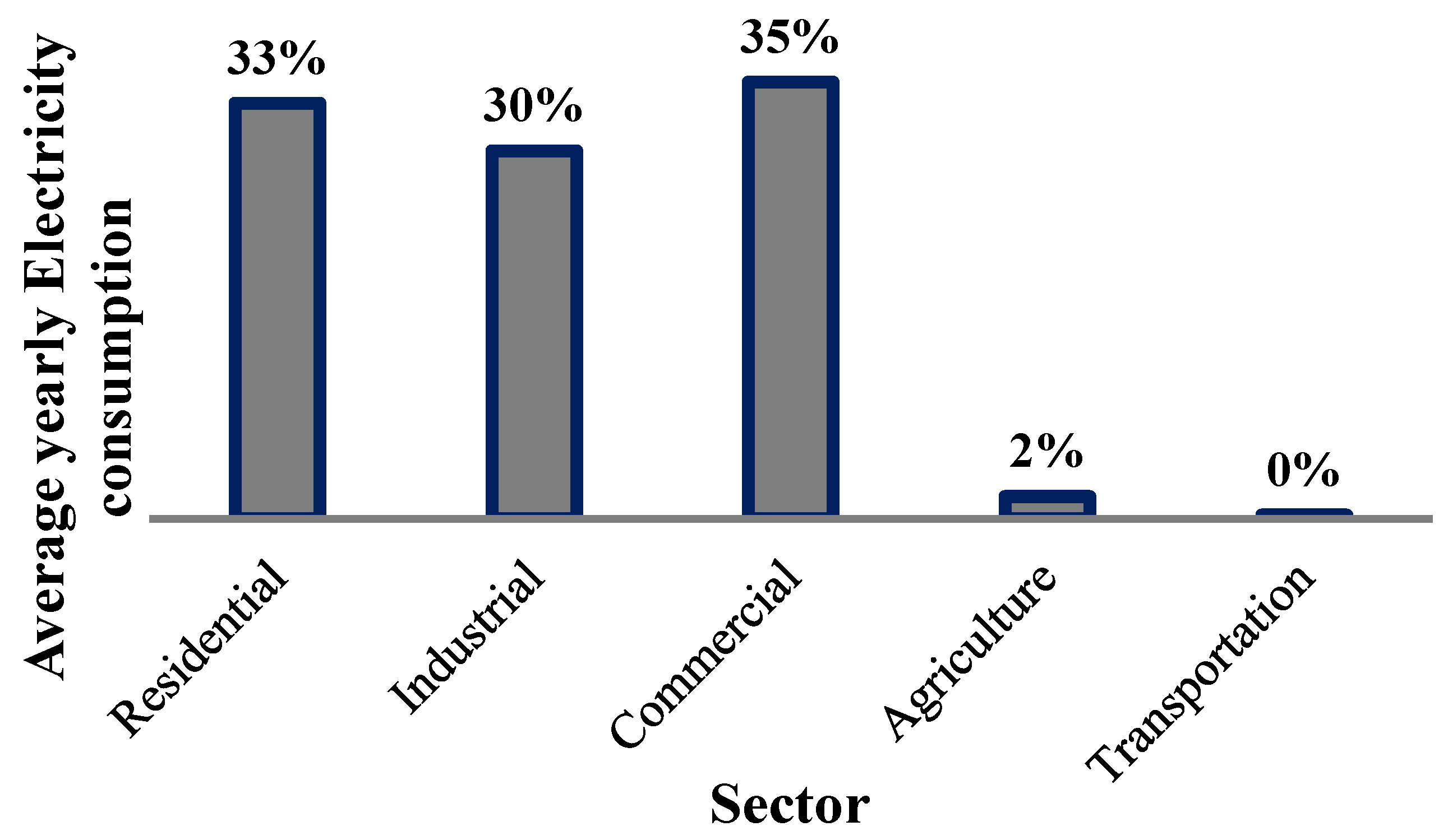
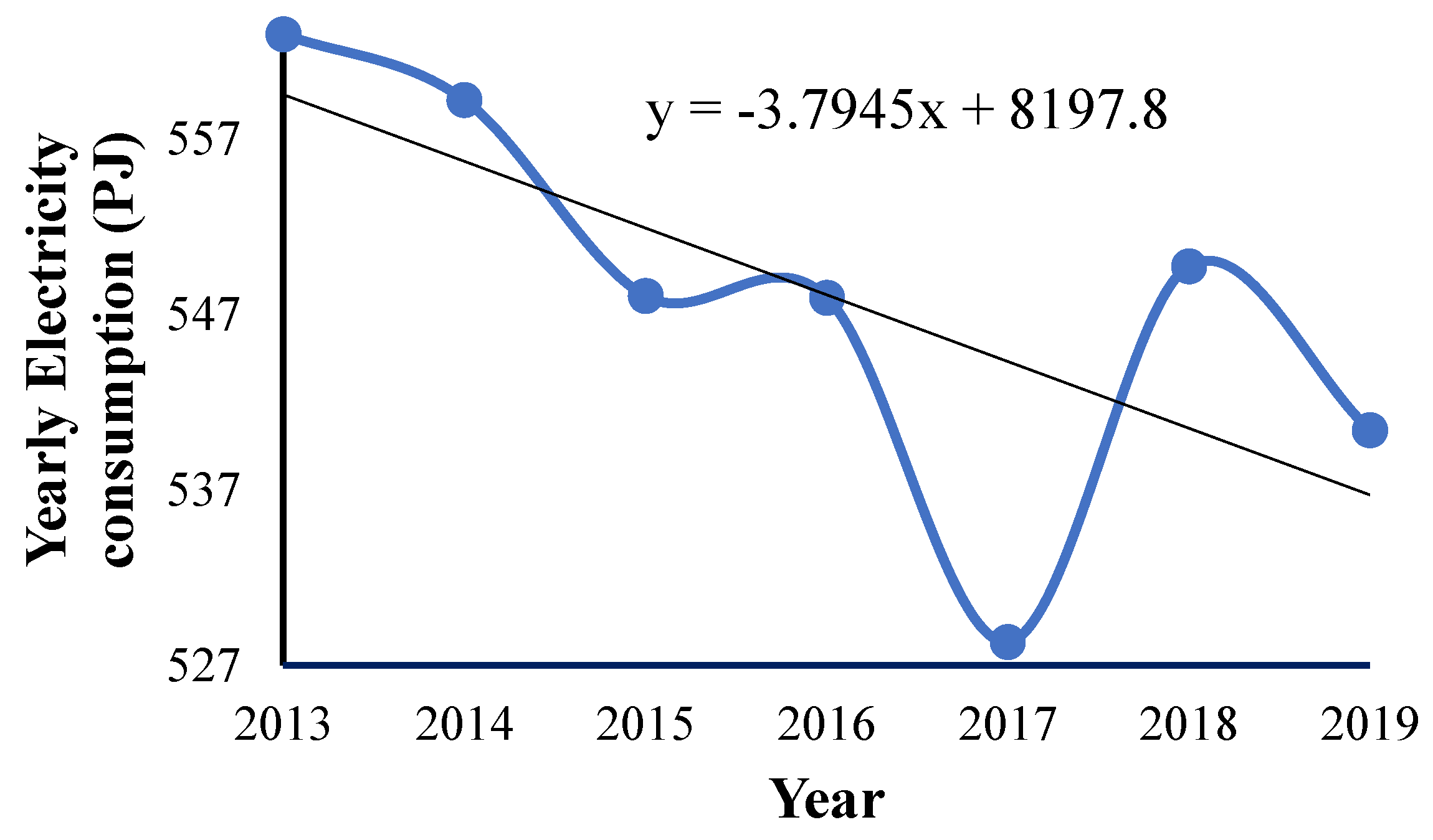
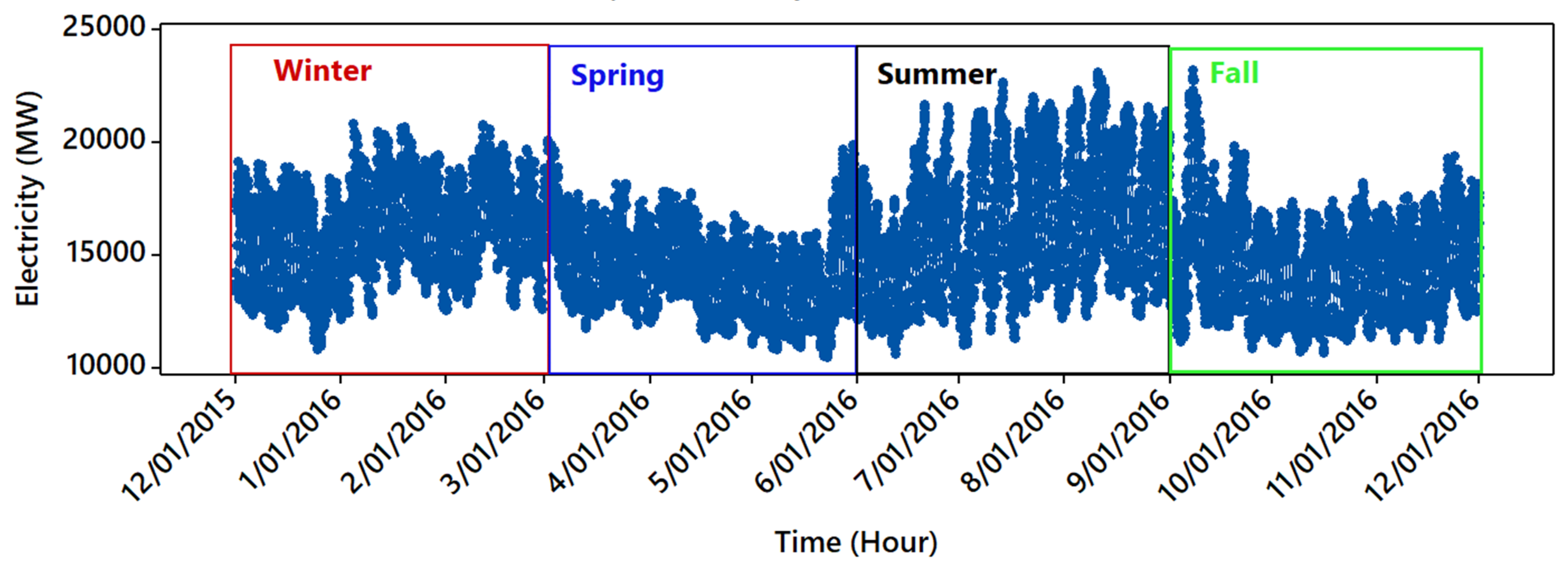
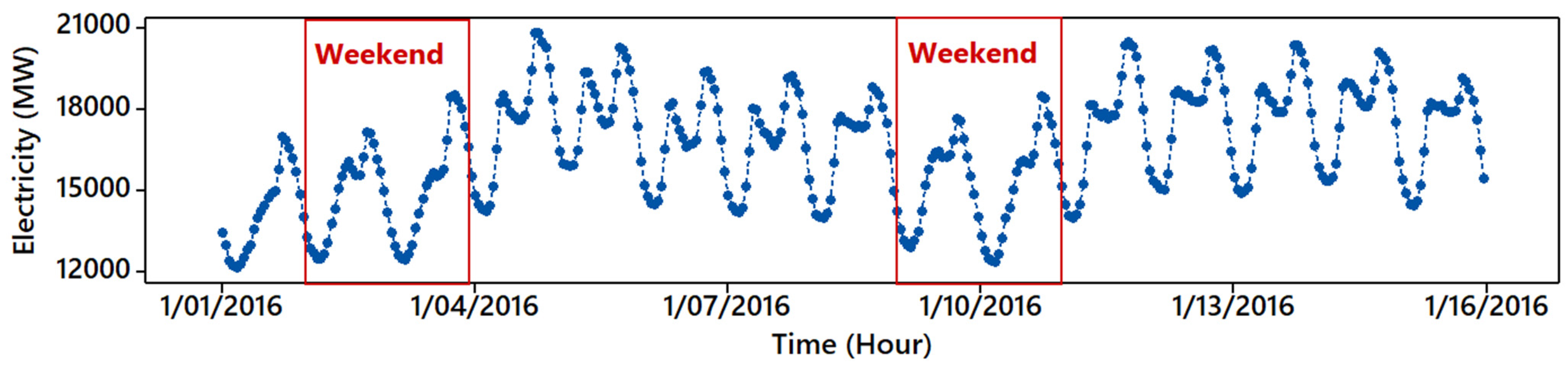
Explore the details of overall electricity consumption in Ontario.

(2)

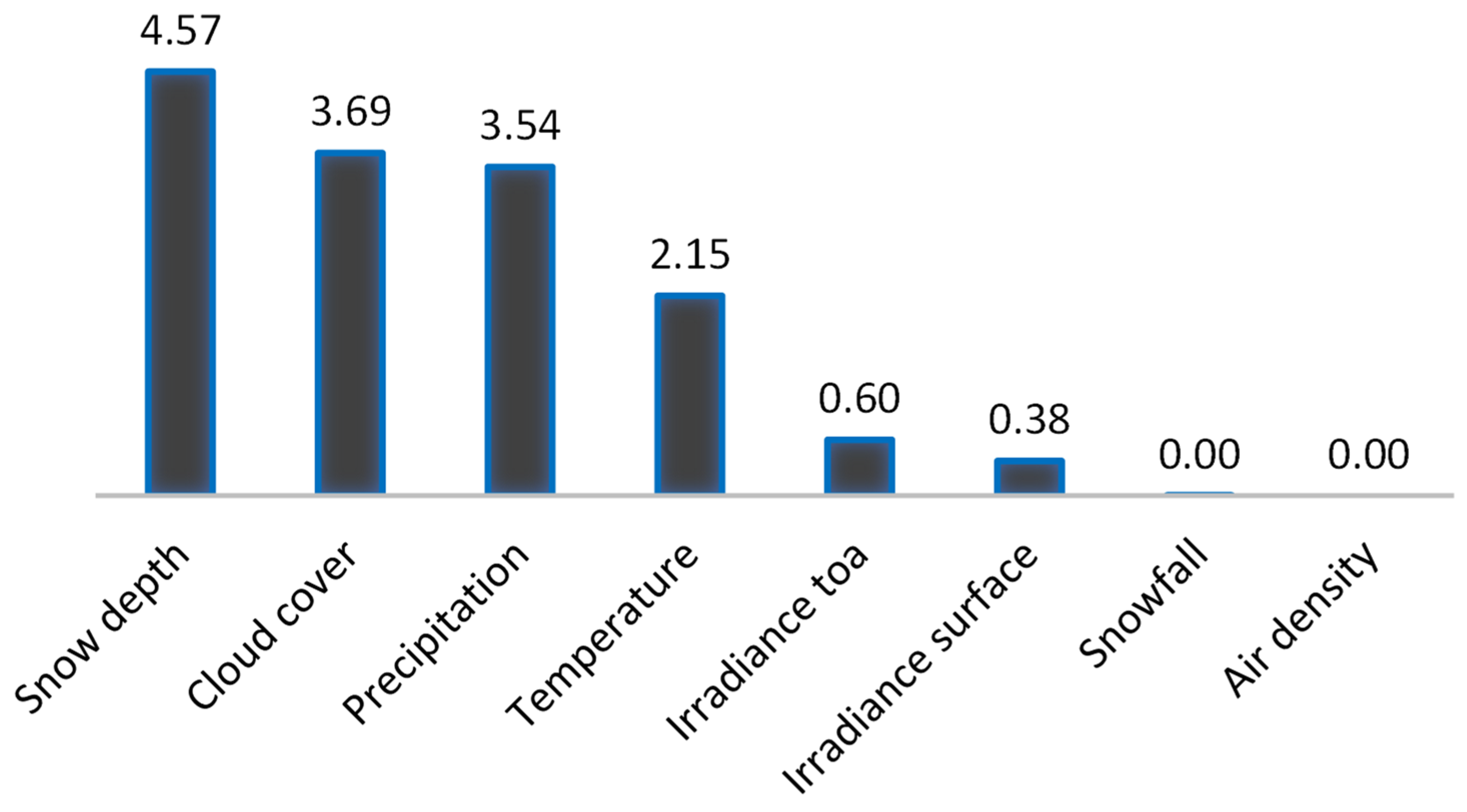
Investigate the factors that have a significant effect on the electricity consumption in residential sectors.

(3)

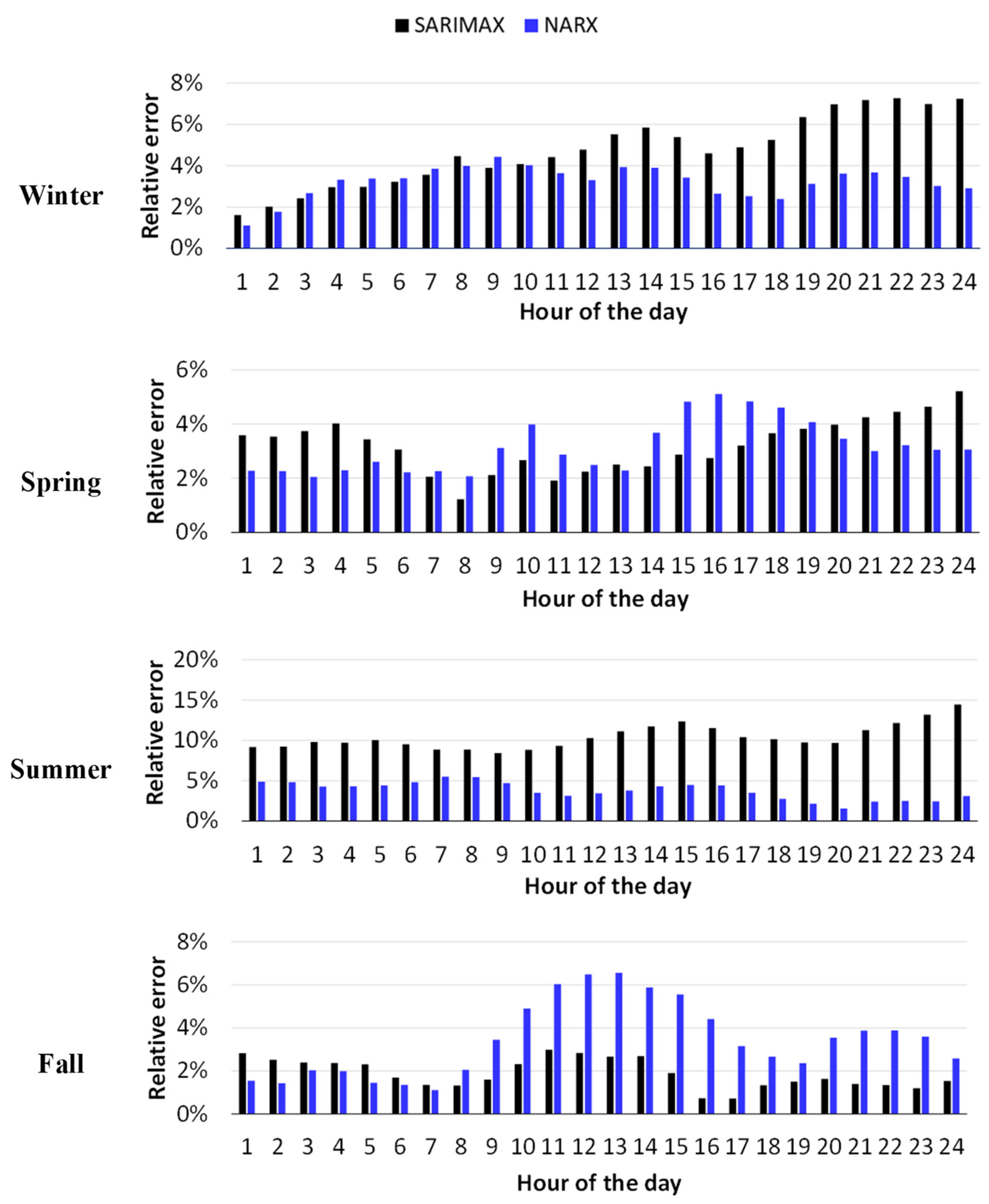
Apply modern data science approaches, namely the seasonal statistical method (SARIMAX) and the machine learning algorithm (NARX), to forecast short-term electricity demand.

(4)

Find the best model by automatic tunning hyperparameters via the Bayesian optimization algorithm (BOA).

(5)

Compare the proposed models using several performance indicators (viz., MAE, RMSE, MAPE, R², adj-R², RE, FB).

(6)

Conduct a robustness analysis to confirm the prediction accuracy of the models.

It is noteworthy that this study marks the first-time use of a hybrid model (BOA-SARIMAX, BOA-NARX) to forecast a short-term electricity demand, especially the hourly forecasting of electricity consumption in Ontario, Canada. Such short-term electrical load forecasting could play a vital role in the power production and scheduling process’s safety, stability, and sustainability.

This paper is structured as follows: Section 2 provides the literature review. The main purpose of this section is to identify and state a clear gap in the current state of knowledge that is being addressed by the developed forecasting method. Section 3 outlines the details of the historical data and the model development process. Section 4 provides details of the results and a discussion. Finally, the concluding remarks are presented in Section 5. To enhance the clarity and readability of the article, all abbreviations have been tabulated in

Table 1. Acronyms used in the article.

Acronym	Description	Acronym	Description
ABCNN	Artificial Bee Colony-based ANN model	LSTM-RNN	LSTM-based Recurrent Neural Networks
ACF	Autocorrelation function	NARX	Nonlinear autoregressive networks with exogenous input
ACS	Artificial cooperative search	MA	moving average
AE	Absolute error	MAE	Mean absolute error
AIM	Abductory Induction Mechanism	MAPE	Mean Absolute Percentage Error
ANN	Artificial Neural Network	MARS	Multivariate Adaptive Regression Spline
ANN ABC	Artificial neural network with artificial bee colony algorithm	ML	Machine learning
ANN BP	ANN with backpropagation	MLP	Feedforward multilayer perceptron structure
ANN TLBO	ANN with Teaching Learning Based Optimization	MLR	Multiple linear regression
APSONN	Artificial Particle Swarm Optimization based ANN	MODWT	Maximum overlap discrete wavelet transform
AR	Autoregressive	MPOE	MODWT-PACF-OS-ELM
ARIMA	Autoregressive integrated moving average	MSE	Mean square error
ARMAX	Autoregressive moving average	MWh	Megawatt-hours
BOA	Bayesian optimization algorithm	NRCan	Natural Resources Canada
CER	Canada Energy Regulator	OPEC	Organization of Petroleum Exporting Countries
CS	Cuckoo Search algorithm	OS-ELM	Online sequential extreme learning machine
CSNN	Cuckoo Search Algorithm utilizing Lévy flights associated with ANN	PACF	Partial autocorrelation function
CVRMSE	Coefficient of variation RMSE	Pj	Yearly electricity load
DE	Differential Evolution	POE	PACF-OS-ELM
ELM	Legates and McCabe’s Index	PSO	Particle-swarm optimization
EMD	Empirical Mode Decomposition	QQ plot	Quantile–quantile plot
ENS	Nash–Sutcliffe efficiency coefficient	R2	Coefficient of Determination
FB	Fractional Bias	R2 (adj)	Adjusted Coefficient of Determination
GA	Genetic algorithm	RE	Relative error
GANN	Genetic Algorithm based ANN	RF	Random Forest
GB	Gradient Boosting	RRMSE	Relative Root Mean Square Error
GP	Gaussian process	RMSE	Root Mean Square Error
HDIP	Hydrocarbon Development Institute of Pakistan	RNN	Recurrent Neural Network
ICA	Independent Component Analysis	SARIMAX	Seasonal autoregressive integrated moving average with exogenous inputs
KNN	K-Nearest Neighbor	SA	Simulated Annealing
LEAP	Long-range Energy Alternative Planning	SVR	Support Vector Machine
LR	Linear Regression	WI	Willmott’s Index
LSTM	Long–short-term memory

.

2. Literature Review

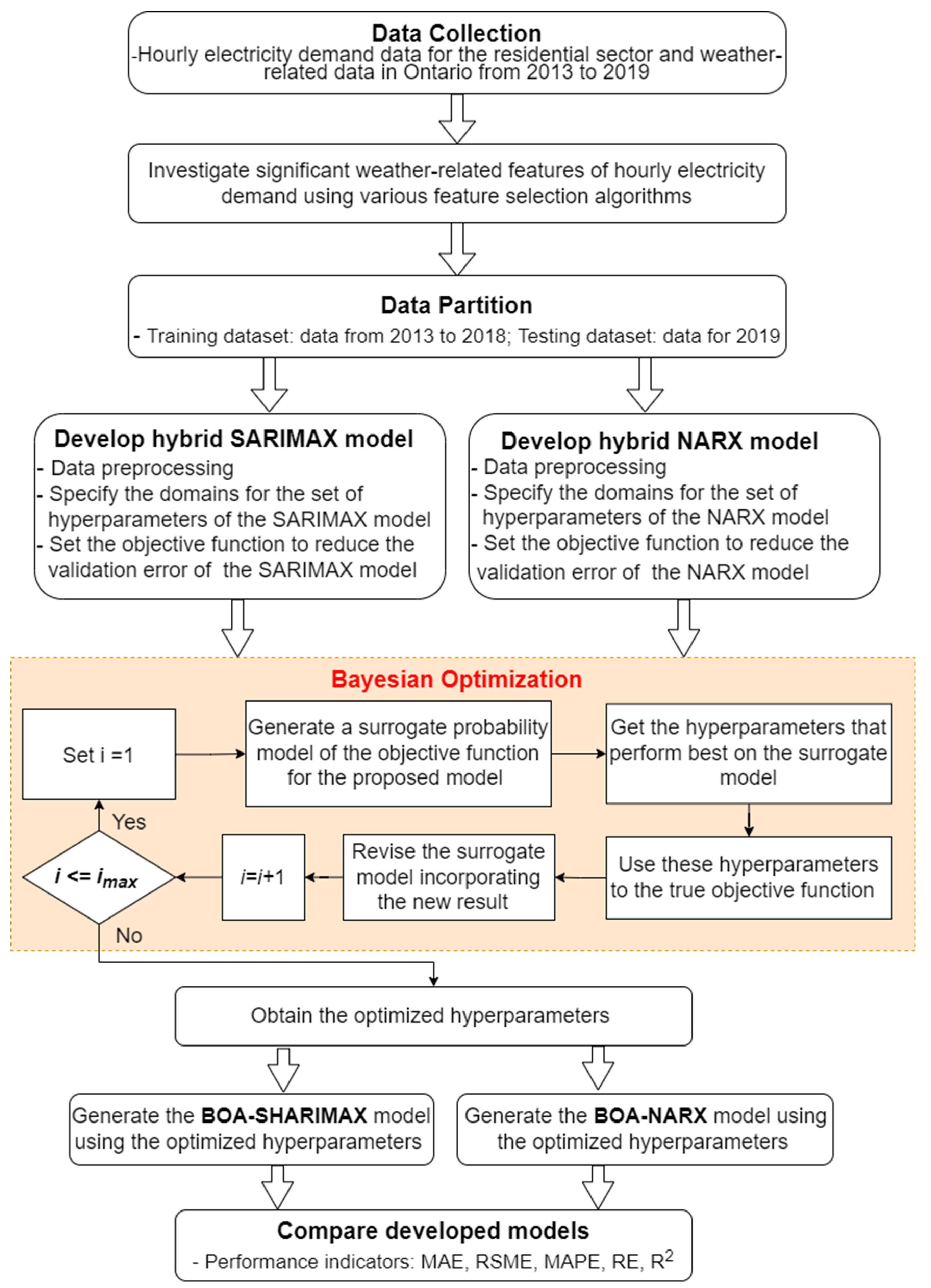
Electricity demand forecasting received deep concern from many researchers in different countries due to its essential contribution to planning and power system management. Numerous studies have been conducted to forecast electricity demand during the past several decades. Various algorithms were used in these studies to achieve the best model performance, in short-, medium-, and long-term electricity demand forecasting.

Aghay Kaboli et al. conducted a study to forecast the long-term electricity demand in Iran using the Artificial Cooperative Search (ACS) approach, a recently developed evolutionary algorithm with a high probability of finding the optimal solution to complex optimization problems [21]. This study involved the socio-economic indicator, namely gross domestic product (GDP), population, import, export, and stock index, which may have a remarkable effect on increasing or decreasing electric energy demand. The annual energy demand data from 1992 until 2013 were used in this study for model development and validation. The authors stated that the developed ACS algorithm is more efficient in forecasting compared with other optimization methods that had been applied for energy consumption forecasting, namely, Genetic Algorithm (GA), Practical Swarm Optimization (PSO), Independent Component Analysis (ICA), Cuckoo Search algorithm CS, Simulated Annealing (SA), and Differential Evolution (DE). In addition, linear, quadratic, exponential, and logarithmic mathematic models were implemented for the path coefficient analysis to detect the best weighting factors. Finally, the results of this study confirmed that ACS achieved high performance in forecasting the electricity demand with the lowest errors measured with the evaluation metrics, namely, Absolute Error (AE), Root Mean Square Error (RMSE), U-statistic, and Mean Absolute Percentage Error (MAPE).

Ur Rehman et al. have applied three energy forecasting models based on the Autoregressive Integrated Moving Average (ARIMA), Holt-Winter, and Long-range Energy Alternative Planning (LEAP) methods to predict the energy consumption of five essential fuels, i.e., electricity, natural gas, oil, coal, and liquefied petroleum gas in six fields, namely domestic, industrial, commercial, transportation, agriculture and other governmental sectors in Pakistan [22]. In [22], the researchers retrieved annual energy data from the Hydrocarbon Development Institute of Pakistan (HDIP) from 1992 until 2014. Later, the study forecasted the energy consumption for the coming 21 years. The ARIMA and Holt–Winter algorithms were used in this study, and the results were tested and validated by RMSE and MAPE. The LEAP software tool was also used in this study to build the forecasting model, which was highly suggested for different applications related to energy demand forecasting at many spatial levels such as cities, states, or countries due to their enormous potential and ability to forecast using minimum data. However, the authors of [22] proved that the ARIMA model was the most appropriate model to predict energy demands with a confidence interval of 95% compared with the other two models.

In [23], Kankal et al. developed models to forecast the electricity demand in Turkey. In that study, the data were retrieved from different local and international resources from 1980 to 2012 to collect data about the independent variables, GDP, population, import, and export. A new optimized algorithm based on Artificial Neural Network (ANN) called ANN-Teaching Learning Based Optimization (ANN-TLBO) was used in this study to develop a forecasting model of electricity demand. This proposed algorithm was inspired by the teaching–learning process, where the effect of an excellent teacher reflects positively on the student performance in the exam, and the effects of students’ interaction among each other also affect their performance. The prediction performance of this proposed algorithm was evaluated by comparing it with the performance of the artificial neural network with backpropagation (ANN-BP) and the artificial neural network with artificial bee colony algorithm (ANN ABC) models. The ANN-TLBO defeated the other two models; the root mean square error (RMSE) was reduced by 42.3% and 39.3%. The authors also stated that the ANN-TLBO algorithm had a significant advantage in decreasing the computational complexity.

In [24], Khan et al. forecasted the electricity consumption in the 12 countries in the Organization of Petroleum Exporting Countries (OPEC), namely Algeria, Angola, Ecuador, Iran, Iraq, Kuwait, Libya, Nigeria, Qatar, Saudi, the United Arab Emirates, and Venezuela. The dataset was collected by yearly electric consumption from 1980 till 2012 to predict the demand 3 years ahead, 6 years ahead, 9 years ahead, and 13 years ahead. The Cuckoo Search Algorithm utilizing Lévy flights associated with the ANN was used in this study to construct the CSNN model for forecasting electricity consumption. For model performance evaluation, the study compared the results of the MSE with other models, namely, the Artificial Particle Swarm Optimization-based ANN model (APSONN), the Genetic Algorithm-based ANN model (GANN), and the Artificial Bee Colony-based ANN model (ABCNN). The results illustrated that CSNN achieved the best performance among the other models.

Some research was conducted to study the forecasting methods for both short and long prediction periods. Yukseltan et al. used the Fourier series expansion in electricity demand forecasting in Turkey [25]. In that study, the researchers applied the feedback-based forecasting methodology to forecast the electricity consumption for the next hour based on the error found in the present hour. The dataset was obtained from 2012 to 2017 and was used to forecast the consumption in an hourly, daily, and yearly manner. A two-year observation period was applied to generate hourly forecasting for the coming year.

Moreover, the last two-year period data were used to predict the coming day and the next hour based on a feedback mechanism. The result of the proposed model achieved a high performance in forecasting the electricity demand, and it was validated by testing the MAPE with 0.87%, 2.90%, and 3.54% in the hourly, daily, and yearly forecasts, respectively. Additionally, the study utilized an autoregressive (AR) model to enhance the predictions by the Fourier series expansion and provide better accuracy.

In [15], Bouktif et al. forecasted the short–medium term electric load in Canada using monthly data retrieved from France metropolitan’s electricity consumption for nine years. The long–short-term memory (LSTM)-based Recurrent Neural Networks (LSTM-RNN) and other machine learning models, namely Linear Regression (LR), Ridge, Regression K-Nearest Neighbours (KNN), Random Forest (RF), Gradient Boosting (GB), and ANN and Extra Trees Regressor, were used in this study. The forecasting performances of the developed models were then compared to identify the best predictive model. Additionally, this study included several features such as time lags, temperature, humidity, wind speed, and schedule-related variables (month number, weekends, weekdays). The genetic algorithm (GA) was used in this study to select the best features and time lags to optimize the model performance. The results showed that LSTM-RNN achieved a better performance in forecasting electricity load than the ML models, with the coefficient of variation RMSE (CVRMSE) of 0.61% for the short term and an average of 0.56% for the medium term.

Several studies focused on developing short-term forecasting models. In [26], Bedi et al. delivered a hybrid model to estimate the short-term electric energy demand forecast in the city of Chandigarh in India. This study used deep learning-based algorithms, namely the long–short-term memory network (LSTM) and Empirical Mode Decomposition (EMD), to develop the proposed hybrid model. The dataset was retrieved for five years (from January 2013 to January 2018) in addition to a recorded electric consumption every 15 min each day to estimate the short-term forecasting. In addition, multiple regression models were applied to compare the results with the proposed hybrid model, such as Recurrent Neural Network (RNN), LSTM, and EMD-based RNN (EMD + RNN) models. RMSE and MAPE were used to evaluate the model performance, and the results showed that the hybrid model (EMD + LSTM) achieved better accuracy than the regression models from 5 to 8%.

In [27], AL-Musaylh et al. aimed to construct an artificial neural network (ANN) model for short-term electricity demand forecasting over other models based on multiple linear regression (MLR), MARS, and ARIMA. The dataset in that study was obtained from July 2014 to June 2017 in around 200 suburbs in Southeast Queensland, Australia. That study included six climate variables, namely maximum temperature, minimum temperature, rainfall, evaporation, solar radiation, and vapor pressure to estimate the daily electricity consumption and six-hour ahead prediction. Further, to evaluate the model performance, the study applied six evaluation metrics, namely Legates and McCabe’s Index (ELM), Willmott’s Index (WI), and Nash–Sutcliffe efficiency coefficient (ENS), MAE, RMSE, MAPE, and RRMSE. The results showed that the ANN model outperformed the other models. Moreover, a hybrid ANN model was developed in that study by merging the forecasts of ANN, MARS, and MLR. This hybrid model’s highest predictions were compared with other models, with the RMSE of 3.85% for the six-hour forecasting and 4.37% for daily forecasting.

Al-Musaylh et al. developed forecasting models utilizing various algorithms, namely Multivariate Adaptive Regression Spline (MARS), Support Vector Regression (SVR), and the statistical (ARIMA) model to forecast the short-term electricity demand in Queensland, Australia [30]. These models predicted the electric energy at 0.5 h ahead, 1.0 h ahead, and 24 h onwards. The dataset used in this study contains electricity consumption from January 2012 to December 2015. This study utilized multiple evaluation metrics for model performance, including the Pearson Product Moment Correlation coefficient (r), RMSE, and MAE. The results illustrated that, by forecasting the short-term horizons of 0.5 h and 1.0 h, the MARS model achieved better performance than the ARIMA and SVR models with MAE values of 0.765 and 1.446, respectively. On the other hand, the SVR model outperforms the other two models in forecasting daily electricity consumption with 2.717 MAE.

K. Chapagain et al. developed short-term electricity demand forecasting models and analyzed the impact of temperature and other deterministic features on the Thai electricity demand [28]. The whole dataset was divided into four subgroups based on demand characteristics, and models were developed for each subset. The feedforward artificial neural network was developed in this study, and the model accuracy was compared with regression methods, namely ordinary least square and general least square. The authors state that regression methods have better forecasting accuracy than the developed feedforward artificial neural network. The authors also found that the temperature is linearly related to the Thai electricity demand. The maximum effect of temperature during the night hours occurs at 11 p.m., is 300 MW/°C, about a 4% rise in demand. However, the temperature impact is only 10 MW/°C to 200 MW/°C during day hours, about a 1.4% to 2.6% rise in demand.

Elnakla et al. compared the electricity demand per capita in Saudi Arabia with the United Arab Emirates (UAE) and Australia [31]. The results showed that Saudi Arabia consumes less electric energy than the UAE and higher electricity than Australia. Moreover, this study forecasted the electricity consumption in Saudi Arabia based on three scenarios. The first scenario was ‘Optimistic’, which estimated the average population growth would be 2.5% per year while the electricity consumption would increase by 1% per year. The second scenario was ‘Moderate’, which assumed that population growth would increase by 3% per year. The third scenario was ‘Pessimistic’, which assumed that the average population growth would continue along the same trend as the previous 40 years and the annual electricity consumption would be the as same as the last 20 years. Further, this study forecasted electricity consumption from 2014 until 2040. The results showed that to provide reliable electricity consumption and ensure availability for all sectors, KSA should increase the electricity generation by 215% based on the ‘Optimistic’ scenario and by 514% to meet the population demand based on the ‘Pessimistic’ scenario.

Abdel-aal et al. forecasted the consumption of electrical energy for the Eastern province of Saudi Arabia based on weather parameters and demographic and economic variables [32]. This study applied a Univariate Box–Jenkins time-series analysis on monthly data for six years from August 1987 to July 1993; the first five years were used to develop the model, while the dataset for the 6th year was used for validating the models. The non-seasonal and seasonal autoregressive models were used in this study. Moreover, different models were developed using the Abductory Induction Mechanism (AIM) and multivariate regression models. The results showed that the ARIMA models had the best forecasting results compared with the AIM and multivariate regression models, with an average percentage error of 3.8% compared to 8.1% and 5.6%, respectively.

In [33], N. Liu et al. constructed two different short-term electricity consumption forecasting models based on the ANN approach and the Seasonal Autoregressive Integrated Moving Average with exogenous variables (SARIMAX) to predict a week ahead of electricity demand. An hourly electricity consumption dataset from 2010 to the middle of 2011 in Abu Dhabi, UAE, was utilized in this study. This study considered the impact of the dry bulb temperature as a variable that affected the electricity load. This study showed that the ANN model reacted better in the estimation stage than the SARIMAX. In contrast, the forecasting results illustrated that SARIMAX outperformed the ANN model with an RMSE of 62.61 MW; the MAPE was 2.98%, while the ANN model achieved an RMSE of 72.92 MW with a MAPE of 3.57%. Thus, the authors concluded that the SARIMAX model is comparatively more reliable and better for this forecasting process.

Similarly, A. Shadkam in [34] applied short-term prediction by using the SARIMAX model to forecast the peak and daily electricity demand in two university buildings in Canada. For that purpose, a daily dataset was obtained about these two buildings from 2017 to 2019. The electricity demand from 2017 to 2018 was used in this study to develop the model, while the data for 2019 was used to test the performance. Additionally, this study included the impact of the daily average temperature and humidity on electricity consumption. Ultimately, the SARIMAX model achieved desirable forecasting results for both buildings. For the first university building, the MAPE was 4.1%, while the second university building reached a MAPE of 12.8%.

J. Buitrago et al. conducted short-term electricity consumption forecasting techniques on the New England electric grid to forecast the next 24 h to enhance the energy load resources and the cost [35]. This study used a nonlinear autoregressive with exogenous multi-variable input (NARX) based on the ANN approach to training the data in an open loop to optimize the results. Then, the forecasting data was generated in a closed loop using the predicted values as the feedback input. An hourly dataset was retrieved from 2005 till 2015, and weather data such as wet bulb temperature and dry bulb temperature were utilized as exogenous. The performance of the proposed model was compared to the ARMAX model, and the results showed that NARX outperformed with MAPE of 0.85% while the ARMAX achieved 1.09%.

M. Al-Musaylh et al. in [36] combined the online sequential extreme learning-machine (OS-ELM) model and the maximum overlap discrete wavelet transform (MODWT) algorithm to forecast the electric demand on three campuses at the University of Southern Queensland, Australia. Daily electricity consumption data was collected for two periods, from January 2013 to December 2014 and September 2015 to August 2016. The authors applied the partial autocorrelation function (PACF) technique to select the most critical lagged input variables in the time series data. Then, the MODWT-PACF-OS-ELM (MPOE) model was compared with the non-wavelet equivalent PACF-OS-ELM (POE) model, and the results illustrated that the MPOE achieved better performance than the POE with a MAPE of 4.31%, while POE scored a MAPE of 11.31%.

Table 2. Comparative table of related studies.

Refs.	Region	Extra Information	Method	Hyperparameters Tuning	Benchmarked Methods	Metrics	Performance
[21]	Iran	Socio-economic indicator	ACS	Linear, quadratic, exponential, and logarithmic mathematic models	GA, PSO, ICA, CS, SA, DE	AE, RMSE, U-statistic, MAPE	ACS achieved high performance with the lowest errors measured
[22]	Pakistan		ARIMA		Holt-Winter	RMSE, MAPE	ARIMA confidence interval of 95% compared with other models
[23]	Turkey	GDP, population, import, and export	ANN-TLBO		ANN-BP, ANN-ABC	RMSE, Time	RMSE reduced by 42.3% and 39.3%
[24]	12 OPEC countries		CSNN		APSONN, GANN, ABCNN	MSE	CSNN achieved the best performance
[25]	Turkey					MAPE	0.87%, 2.90%, and 3.54% in the hourly, daily, and yearly forecasts
[15]	France	Time lags, temperature, humidity, wind speed	LSTM-RNN	GA	LR, Ridge regression, KNN, RF, GB, ANN, Extra tree regressors	RMSE	Variation of 0.61%
[26]	Chandirgah/India		Hybrid LSTM and EMD		RNN, LSTM. EMD + RNN	RMSE, MAPE	Better accuracy + 5 to 8%
[27]	Southeast Queensland, Australia	Maximum temperature, minimum temperature, rainfall, evaporation, solar radiation, and vapor pressure	Hybrid ANN + MARS + MLR		ANN, MLR, MARS, ARIMA	ELM, WI, ENS, MAE, RMSE, MAPE, RRMSE	RMSE of 3.85% for the 6 h forecasting and 4.37% for daily forecasting
[30]	Queensland, Australia		MARS		ARIMA, SVR	r, RMSE, MAE	MAE values of 0.765 and 1.446, respectively
[28]	Thailand	Temperature and other deterministic features on Thai electricity demand	Feedforward artificial neural network		ordinary least square and general least square		Regression had better accuracy
[32]	Eastern province of Saudi Arabia	Weather parameters and demographic and economic variables	ARIMA (univariate Box-Jenkins time-series analysis)		AIM, multivariate regression	Average percentage error	Average percentage error of 3.8% compared to 8.1% and 5.6%
[33]	Abu Dhabi, UAE	Dry bulb temperature as a variable that affected the electricity load	SARIMAX		ANN	RMSE, MAPE	SARIMAX outperformed ANN with RMSE of 62.61 MW (vs. 72.92 MW), MAPE 2.98% (vs. 3.57%)
[34]	Two university buildings in Canada	Daily average temperature and the humidity	SARIMAX			MAPE	4.1% and 12.8%
[35]	New England electric grid	Wet bulb temperature and dry bulb temperature)	NARX		ARMAX	MAPE	NARX MAPE = 0.85% vs. ARMAX MAPE = 1.09%
[36]	Three campuses in the University of Southern Queensland, Australia		MPOE		POE	MAPE	4.31%
This study	Ontario, Canada	Precipitation, snowfall, snow mass, air density, ground-level solar irradiation, top of atmosphere solar irradiation, cloud cover fraction	NARX	BOA	SARIMAX	MAE, RMSE, MAPE, R2, RE, time	BOA-NARX MAPE ~3%, steady RE 1~6.56%)

summarizes the related studies in their region of application, the available extra information, the developed method, whether hyperparameter tuning was performed, the benchmarked methods, and comparison metrics. One can observe that no study focuses on data from Ontario, Canada. Most of the studies benefitted from extra information, especially weather information. Very few studies utilized optimization techniques to efficiently tune their hyperparameters, though it is known that this is a significant bottleneck in the forecasting pipeline; furthermore, none of these studies investigated BOA. Various machine learning, deep learning, and evolutionary methods have been utilized for benchmarking purposes. Moreover, a wide range of metrics is being used for comparison, with some studies using only one metric. However, only one study also considered time complexity. On the other hand, the last row of this table lists the features of our study, clearly highlighting the novelty of this study; it is the first study investigating short-term load forecasting in Ontario, including significant weather data, developing a novel hybrid method based on NARX (shown to be promising in [35]) and BOA for hyperparameters optimization, benchmarked with SARIMAX (another promising method as shown in [28,34]), based on a wide range of metrics, including time complexity.

3. Methodology

This section first presents a description of the dataset used in this study and some fundamental statistical analyses. Afterward, the proposed algorithms’ brief mathematical background and operational principles are described. This section also summarizes the Bayesian algorithm’s mathematical formulation and theoretical principles and optimizes the proposed algorithms’ hyperparameters. Figure 2 outlines the major steps of the methodology adopted in this study.

3.1. Data Description

Hourly electricity demand data for the residential sector of the Ontario province of Canada from 2013 to 2019 was used in this study. Data were collected from Natural Resources Canada (NRCan). The hourly air temperature and weather data (precipitation, snowfall, snow mass, air density, ground-level solar irradiation, top of atmosphere solar irradiation, cloud cover fraction) were collected from ETH Zurich and Imperial College London. An overall decreasing trend was observed in the yearly electricity (PJ) load from 2013 to 2019 (see Figure 3). Note that a decreasing demand is usually uncommon, but Ontario is notorious for energy conservation efforts as well as improvements in energy efficiency. The seasonal effect was analyzed on this dataset. A strong seasonality effect was observed, with high Summer consumption periods, comparatively less winter consumption, and low consumption periods in spring and fall (see Figure 4).

According to NRCan, space heating accounts for 63% of the energy used in the average Canadian home and 56% of the energy used in commercial settings. However, electricity consumption is less in winter than in Summer because oil/gas is used mainly for space heating based on Canada’s Energy Efficiency Regulations. Based on the daily electricity load analysis, it is observed that the load is lower on weekends compared to weekdays (see Figure 5). Furthermore, daily variations are more significant in periods of high average consumption (see Figure 5). For heating and cooling purposes, electricity consumption has strong temperature dependence or, more precisely, is dependent on deviations from comfortable temperatures.

3.2. Computational Techniques

In this study, both the statistical approach (SARIMAX) and the machine learning approach (NARX) were utilized to forecast Ontario’s hourly electricity demand. MATLAB (version R2021a) was applied for model development and data analysis.

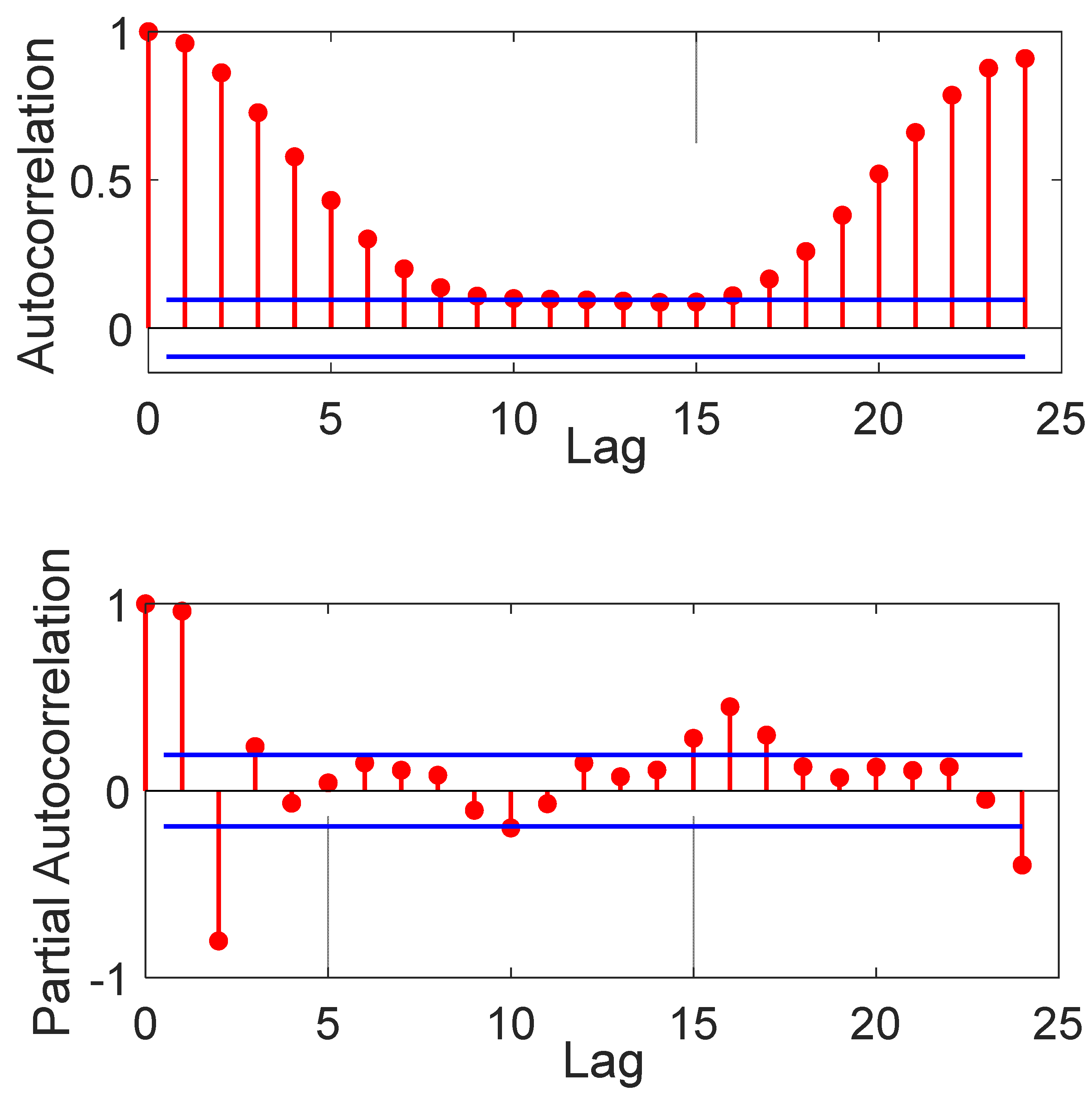
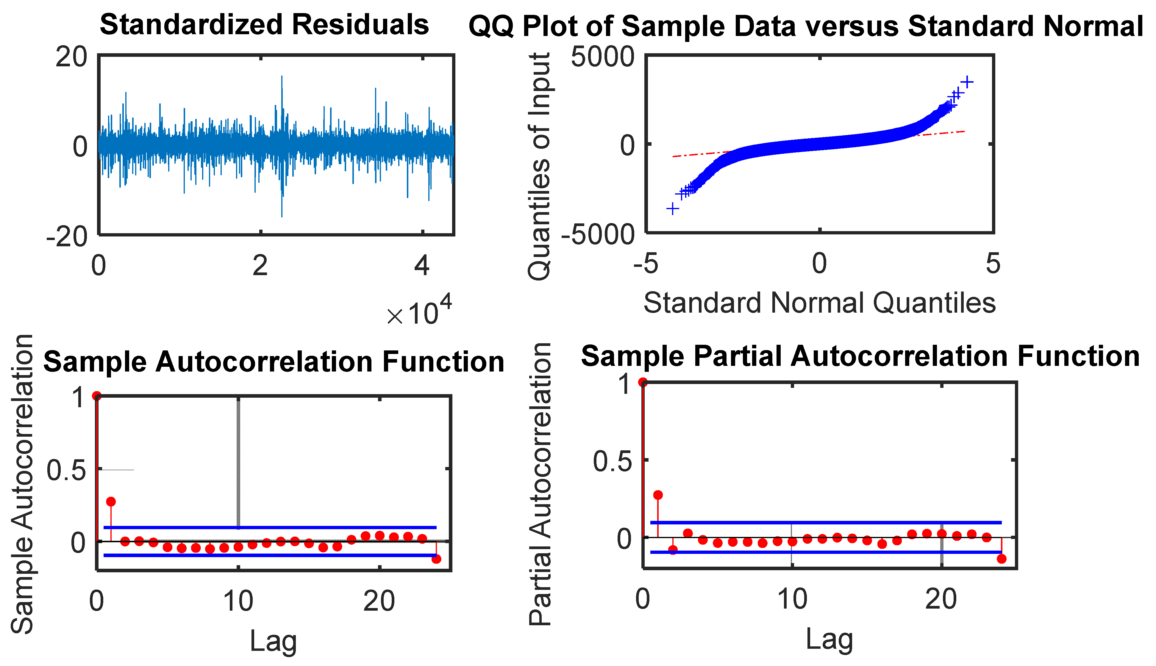
3.2.1. Statistical Approach (SARIMAX)

The Auto-Regressive Integrated Moving Average (ARIMA) model was developed to analyze non-stationary time series that exhibit a particular trend. It is considered one of the most general time series models. The standard ARIMA (p, d, q) linear time series model for a univariate response process $y_t$ can be written as:

$$\left(1-{\displaystyle \sum }_{i=1}^p{\varnothing }_i{B}^i\right){\left(1-B\right)}^d{y}_t=\left(1+{\displaystyle \sum }_{i=1}^q{\theta }_i{B}^q\right)a_t$$

(1)

where $B$ is backshift operator defined as $B{y}_t=y_{t-1}$, $B^j{y}_t=y_{t-j}$, p is the non-seasonal auto-regressive (AR) order, d is non-seasonal differencing, q is the non-seasonal moving average (MA) order, and $a_t$ is the white noise. The values of p and q can be estimated using the sample autocorrelation function (ACF) and partial autocorrelation function (PACF) plots. The ACF describes how the current value of a time series is compared with the previous values. The x-axis is represented by the correlation coefficient, while the number of lags is represented on the y-axis. While the PACF provides the partial correlation between the time series and its lagged values.

The main difference between them is that the PACF plot regressed the time series values at all smaller delays, while the ACF, on the other hand, does not account for additional delays. It is essential to look for significant lags where the autocorrelation and partial autocorrelation values in the ACF and PACF plots exceed the confidence interval. The significant lags can be considered when determining the value of the parameters p and q. Due to the fact that real-time series do not perform like flawless autoregressive models, the estimations supplied by the ACF and PACF plots can only be noticed as a hint.

In addition to non-stationary behavior, many time series show seasonal behavior. The energy demand data usually show intra-day, intra-week, and intra-year seasons. The SARIMA model combines two ARIMA models, one for the base time series and the other for describing the seasonality. The SARIMA model or ARIMA(p, d, q) × (P, D, Q)_s can be described as

$$\left(1-{\displaystyle \sum }_{i=1}^p{\varnothing }_i{B}^i\right){\left(1-{\displaystyle \sum }_{i=1}^P{\mathsf{\Phi }}_i{B}^i\right)}^s{\left(1-B\right)}^d{\left(1-B^s\right)}^D{y}_t=\left(1+{\displaystyle \sum }_{i=1}^q{\theta }_i{B}^q\right){\left(1+{\displaystyle \sum }_{i=1}^Q{\mathsf{\Theta }}_i{B}^Q\right)}^s{a}_t$$

(2)

where ${\left(1-{\displaystyle \sum }_{i=1}^P{\mathsf{\Phi }}_i{B}^i\right)}^s{\left(1-B^s\right)}^D{y}_t={\left(1+{\displaystyle \sum }_{i=1}^Q{\mathsf{\Theta }}_i{B}^Q\right)}^s{a}_t$ represents the seasonal part with parameters P (seasonal AR order), Q (seasonal MA order), D (seasonal differencing), and S (a period of the repeating seasonal pattern).

However, energy forecasts depend on exogenous effects, and including these dependencies may help increase the model’s accuracy. The SARIMAX model permits exogenous parameters by additively or multiplicatively adding a term for the exogenous variable to the equation. This model can be written as below:

$$\left(1-{\displaystyle \sum }_{i=1}^p{\varnothing }_i{B}^i\right){\left(1-{\displaystyle \sum }_{i=1}^P{\mathsf{\Phi }}_i{B}^i\right)}^s{\left(1-B\right)}^d{\left(1-B^s\right)}^D{y}_t=\left(1+{\displaystyle \sum }_{i=1}^q{\theta }_i{B}^q\right){\left(1+{\displaystyle \sum }_{i=1}^Q{\mathsf{\Theta }}_i{B}^Q\right)}^s{a}_t+\left(1+{\displaystyle \sum }_{i=1}^b{\mathsf{\eta }}_i{B}^b\right)d_t$$

(3)

where ${\eta }_i$ are the parameters of the exogenous time series $d_t$ and $b$ is the order of this time series.

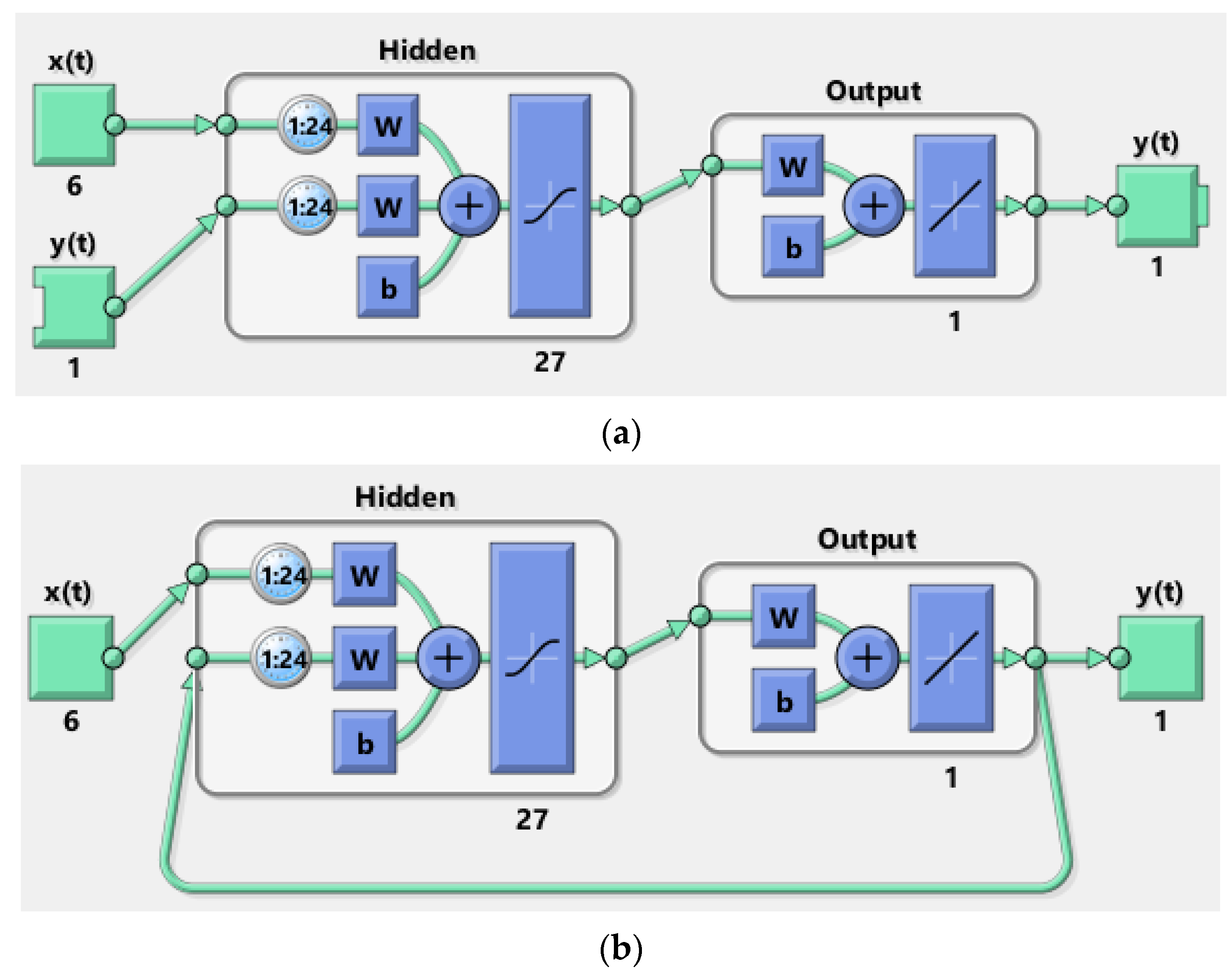
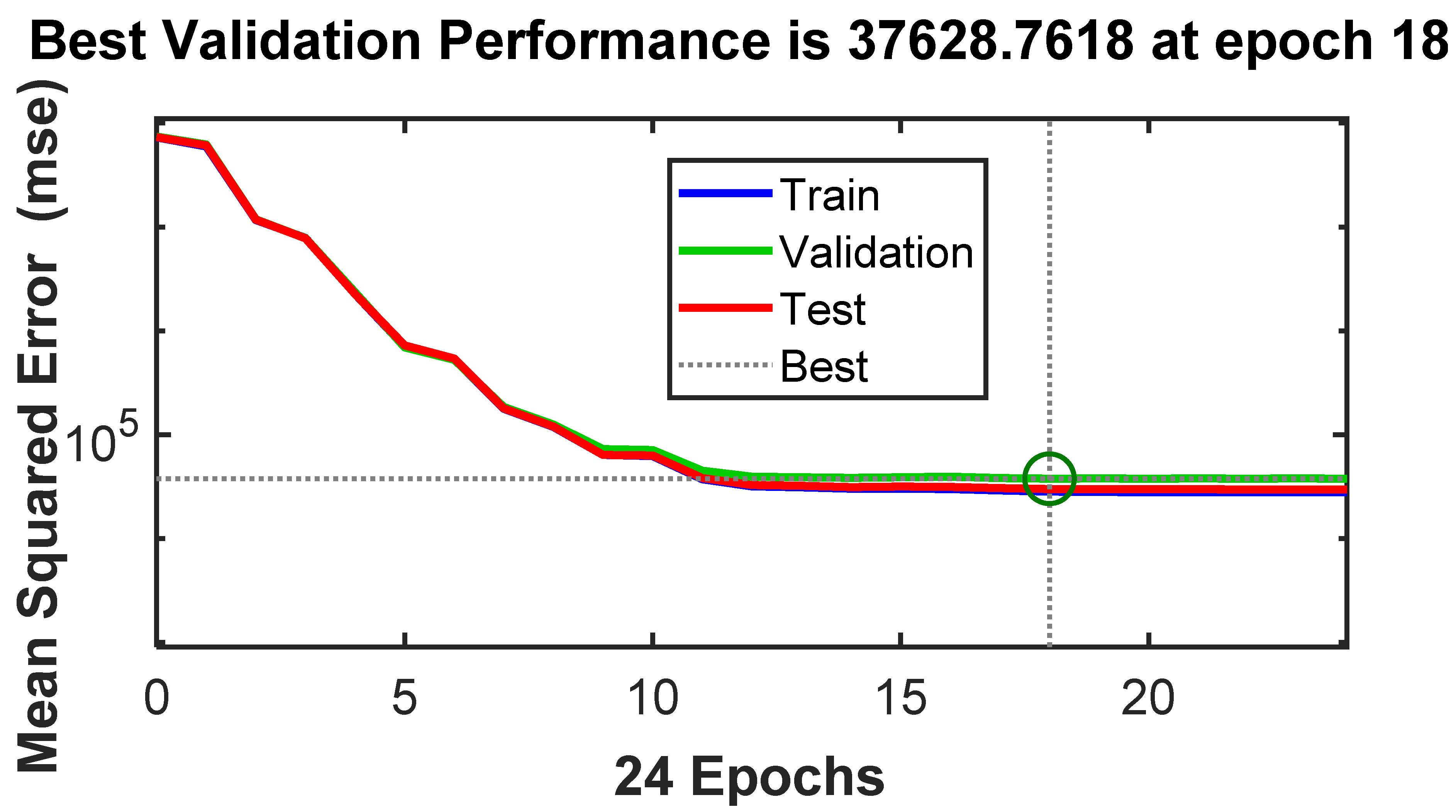
3.2.2. Machine Learning Approach (NARX)

Artificial Neural Networks (ANNs) have been adapted and applied in various applications such as classification, prediction, and recognition due to their structure, which stimulates the brain’s biological neural system and provides a strong ability to learn, store, and analyze data [37,38,39]. ANNs consist of multiple layers, including input, output, and hidden layers that generate mathematical models based on prior knowledge. ANNs can be classified based on the information-flow direction. In feedforward neural networks, nodes are assembled in layers, where inputs are fed to the input layer and passed via hidden layers to the final output layer. On the other hand, information flows forward and backward in recurrent neural networks (RNNs). The output of RNNs is recycled as the next time-step input. The nonlinear autoregressive network with exogenous inputs (NARX) is a recurrent neural network (RNN), which offers the popular feedforward multilayer perceptron structure (MLP) by a global feedback connection between input and output layers. The NARX networks merge ANNs with autoregressive models with exogenous input (ARX), a well-known statistical approach for time series analysis and modeling. These collective features of NARX permit acquiring nonlinear characteristics in an autoregressive time series. The nonlinear autoregressive models with exogenous input relate the current value of the target time series to past values of the same time series and current and past values of other exogenous time series. NARX is frequently applied for nonlinear time series predictions and nonlinear filtering tasks [35,40]. Similar to different types of RNNs, NARX also has limitations in acquiring long-term dependencies due to the trouble of disappearing and shattering gradients. However, they can preserve information up to three times longer than simple RNNs. As a result, they can converge more rapidly and generalize better in comparison [41,42,43,44].

The NARX neural network can be represented mathematically as follows [37,45,46]:

$$y\left(t\right)=f\left[y\left(t-1\right), y\left(t-2\right), . . . , y\left(t – d_y\right), u\left(t-1\right), u\left(t-2\right), . . . , u\left(t – d_u\right)\right]$$

(4)

In Equation (4), $y\left(t\right)$ denotes the target time series, $u\left(t\right)$ indicates the exogenous time series, $d_y$ is the delay of the target variable (known as feedback delay), $d_u$ is the delay of exogenous time series (known as input delay), and $f$ is a nonlinear mapping function of the neural network, which is typically not known (black-box function). This black-box function $f$ passes the input and exogenous time series through a specific number of hidden layers, and certain algorithms train the NARX network to build the best correlation between the inputs and the target variables.

The NARX neural network model architecture consists of two phases: series-parallel architecture (open-loop) and parallel architecture (closed-loop). In the open loop, the training phase contains all the historical data of the variables that will be utilized to determine the node weights and calculate the output to feed the input of the feedforward network. Thus, all training is performed in an open loop, including the validation and testing steps. In addition, only when the network has been trained (which includes validation and testing steps), is it transformed to a closed loop for multistep-ahead prediction, where the actual output is excluded. The predicted delayed output is considered to provide the forecast [35,37].

3.2.3. Hyperparameters Optimization for SARIMAX and NARX

Proper selection of the hyperparameters of SARIMAX (p, q, d, P, Q, D) and NARX (number of hidden layers, number of neurons in each hidden layer, input delay, feedback delay) ensures the model’s prediction performance. The Bayesian optimization algorithm (BOA) was applied in this study to tune the hyperparameters since it provides the best hyperparameters that generate the lowest validation error. In this respect, the BOA was hybridized with SARIMAX and NARX separately to automatically find the optimum values of the hyperparameters.

The BOA is a sequential design procedure for the global optimization of black-box functions with no mathematical differentiation [47]. This optimization framework effectively uses the complete historical data to enhance the search efficiency, and its most important theory is to constantly forecast the posterior information through prior knowledge [19]. The proposed BOA-based optimization approach is more appreciable than other frequently applied optimization techniques, such as grid search, manual search, and random search, depending on its meaningful advantage of utilizing the acquisition function [48]. In particular, the Bayesian optimization approach firstly presumes a functional association between the hyperparameters and the loss function as:

$$h^{\ast }=\arg \underset{hϵH}{\min }loss\left(h\right)$$

(5)

where $H$ denotes the set of hyperparameters, $h$ indicates the set of hyperparameter combinations in $H$, $h^{\ast }$ denotes the optimal combination of hyperparameters achieved from the final optimization, and $loss(•)$ indicates the objective function required to be optimized. The objective function is the validation error of a predictive model and can be described as:

$$loss\left(h_j\right)=\frac{1}{n}{\displaystyle \sum }_{i=1}^n\left|\widehat{y_i}\left(h_j\right)-y_i\right|$$

(6)

where $h_j$ is the $j$th hyperparameter combination, and $y$ is the true value, $\widehat{y}\left(h_j\right)$ is the model outputs obtained using $h_j$.

The following process of BOA is creating a surrogate probability model based on Bayes’ rule to contract the data set $D=\left(h_i,loss\left(h_i\right)\right)$. Here, $h_i$ is the $i$th set of hyperparameters. In this process, a prior distribution $H\left(loss\right)$ combined with the likelihood function $H\left(D|loss\right)$ is used to obtain the posterior distribution $H\left(loss| D\right)$ as the following [19]:

$$H\left(loss| D\right)=H\left(D|loss\right)\ast H\left(loss\right)$$

(7)

The posterior probability approximates the objective function, called the surrogate objective function, and can direct future sampling. The Gaussian process (GP) can be used as a prior for the observed and unknown values of the loss function. A GP extends the multivariate Gaussian distribution to an infinite-dimension stochastic process for which any finite combination of dimensions will be a Gaussian distribution. Similar to a Gaussian distribution, a GP is a distribution over functions entirely specified by its mean function $\mu$ and covariance function $K$ as $f\left(\mathrm{x}\right)\sim \mathrm{GP}\left(\mu \left(\mathrm{x}\right), \left(\mathrm{x},{\mathrm{x}}^{\prime }\right)\right)$. The GP can be considered as a function, but it returns the mean and variance of a normal distribution over the possible values of $f$ at $\mathrm{x}$ instead of returning a scalar $f\left(\mathrm{x}\right)$ for an arbitrary $\mathrm{x}$. When using the Gaussian process for Bayesian optimization, it is assumed that the domain of the Gaussian process is the space of hyperparameters.

To sample efficiently, Bayesian optimization uses an acquisition function, a mathematical technique that guides how the parameter space should be explored during the BOA process. The acquisition function uses the predicted mean and variance generated by the Gaussian process model. Generally, acquisition functions are described such that high acquisition corresponds to potentially high values of the objective function, whether because the forecasting is high, the uncertainty is high, or both. Augmenting the acquisition function is utilized to take the next point to assess the objective function. Thus, the next observation is chosen using the acquisition function as follows:

$$h^{\ast }=\arg \underset{hϵH}{\max }a\left(h|D\right)$$

(8)

where $a(•)$ is the generic symbol for an acquisition function. For more details on the Bayesian optimization, readers are referred to articles published elsewhere [13,14,49,50].

3.2.4. Performance Evaluation Metrics

It is essential to apply multiple statistical metrics to assess the model’s accuracy, because it may perform well with one statistical metric but perform poorly with another indicator. Five performance evaluation metrics are calculated using the following equations to evaluate the performance of the constructed models.

$$\mathrm{Mean} \mathrm{absolute} \mathrm{error} \left(\mathrm{MAE}\right)=\frac{1}{n}{\displaystyle \sum }\left|Av-Pv\right|$$

(9)

$$\mathrm{Root} \mathrm{Mean} \mathrm{Square} \mathrm{Error} \left(\mathrm{RMSE}\right)=\sqrt{\frac{{\displaystyle \sum }{\left(Av-Pv\right)}^2}{n}}$$

(10)

$$\mathrm{Mean} \mathrm{Absolute} \mathrm{Percentage} \mathrm{Error} \left(\mathrm{MAPE}\right)=\frac{1}{n}{\displaystyle \sum }\frac{\left|A_v-P_v\right|}{\left|A_v\right|}\ast 100$$

(11)

$$\mathrm{Coefficient} \mathrm{of} \mathrm{Determination} \left({\mathrm{R}}^2\right)={\left(\frac{{\displaystyle \sum }X Y}{n {\sigma }_x{\sigma }_y}\right)}^2$$

(12)

$$\mathrm{Relative} \mathrm{Error} \left(\mathrm{RE}\right)=\frac{A_v-P_v}{A_v}$$

(13)

$$\mathrm{Fractional} \mathrm{Bias} (\mathrm{FB})=\frac{2{{\displaystyle \sum }}_{i=1}^n\left(Av-Pv\right)}{{{\displaystyle \sum }}_{i=1}^n\left(Av+Pv\right)}$$

(14)

where $n$ is the number of data points, $Y$ is the datasets of the dependent variable, $X$ is the datasets of explanatory variables, ${\sigma }_x$ is the standard deviation of dataset $X$, ${\sigma }_y$ is the standard deviation of dataset $Y$, $A_v$ is the actual value of the data point, and $P_v$ is the predicted value of the data point.

4. Results and Discussions

The hourly electricity consumption data on weekdays from 2013 to 2018 was used to train the model, and the model was tested on 2019 data to examine the forecasting errors and avert overtraining. Initially, eight weather-related features were included in this study. Several feature selection techniques, including univariate feature ranking for regression using F-tests, sequential feature selection, and neighborhood component analysis, were used to select the most relevant and significant features of electricity consumption. The best result was obtained from the neighborhood component analysis (see Figure 6). It is evident that snowfall and air density are not relevant features, as the weights for these two features are very close to zero. The other six features (namely snow depth, cloud cover, precipitation, temperature, irradiance toa, and irradiance surface) are relevant and are considered in this study to develop the predictive models.

4.1. Development of Hybrid BOA-SARIMAX Model

The performance of the SARIMAX model depends intensely on its hyperparameters. Thus, the proper selection of hyperparameters is a pivotal task in getting an optimized model. The ACF and PACF plots of the hourly electricity consumption series were analyzed to determine the value of the parameters p and q (see Figure 7). However, as shown in Figure 7, there is no direct indication of the significant lags that can be used for selecting the value of the parameters p and q. Therefore, the BOA was hybridized with the SARIMAX to determine the optimum value of the hyperparameters [13,14]. As a result, a hybrid BOA-SARIMAX model was developed. Based on the ACF, PACF, and the time series plots of the hourly electricity consumption series, the range [1, 24] was selected for both the p and q, [1, 2] was selected for both P and Q, and [0, 2] was selected for both d and D. The optimum values for p, q, P, Q, d, and D were found to be 24, 14, 2, 2, 0, and 1, respectively (see

Table 3. Optimized hyperparameters of the developed models.

Model
SARIMAX	Parameters	$p$	$q$	$d$	$P$	$Q$	$D$	$S$
	Range for BOA	[1, 24]	[1, 24]	[0, 2]	[1, 2]	[1, 2]	[0, 2]	-
	Optimized value	24	14	0	2	2	1	24
NARX	Parameters	No. of Hidden layers	Hidden layer size	Input delay	Feedback delay	Training function	Training error
	Range for BOA	-	[1, 50]	[1, 24]	[1, 24]	-	-
	Optimized value	1	27	24	24	Levenberg–Marquardt	MSE

). These tuned parameters were used to determine the optimal SARIMAX model. The goodness of fit of the developed BOA-SARIMAX model was assessed by analyzing the residual diagnostic plots (see Figure 8). The quantile–quantile plot (QQ-plot) in Figure 8 shows no apparent violations of the normality assumption. Further, the sample autocorrelation function (ACF) and partial autocorrelation function (PACF) plots for the standardized residuals indicate no significant autocorrelation, confirming that the residuals are uncorrelated.

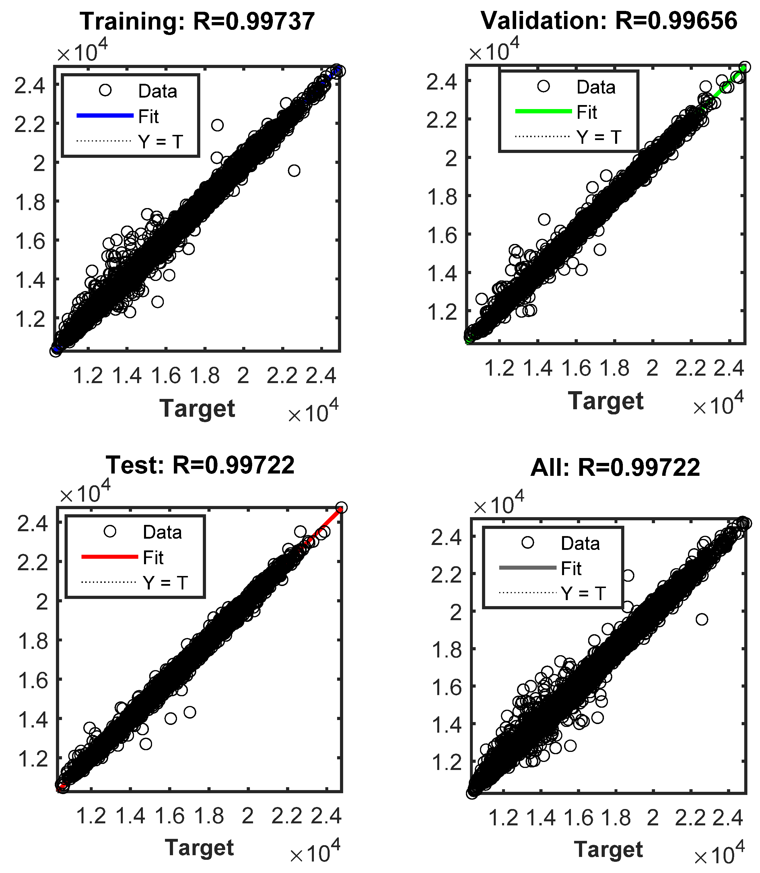
4.2. Development of Hybrid BOA-NARX Model

The BOA was hybridized with NARX to develop the hybrid BOA-NARX model and find the optimal hyperparameters with the simplest structure. In this regard, the number of hidden layers, hidden layer size, input delay, feedback delay, and training function were tuned using the BOA. The optimized hyperparameters of the best predictive NARX model are presented in Table 3, and the network structure is displayed in Figure 9. The performance plot (MSE versus epoch) of the developed NARX model is shown in Figure 10. Generally, in each epoch, the neurons’ weight values were revised. A high epoch value results in high computing times for training, testing, and validating [13]. The training involving adaptive weight minimization halted at the 18th epoch, with the best validation performance of 37,628.7618 (see Figure 10). The errors for both the test and the validation data have similar characteristics, suggesting no overfitting. The regression plots of the developed network based on the training, testing, validation, and whole dataset were used to analyze the goodness of fit (shown in Figure 11). The values of R > 0.99 for all cases suggest a reliable and high predictive performance of the developed NARX neural network.

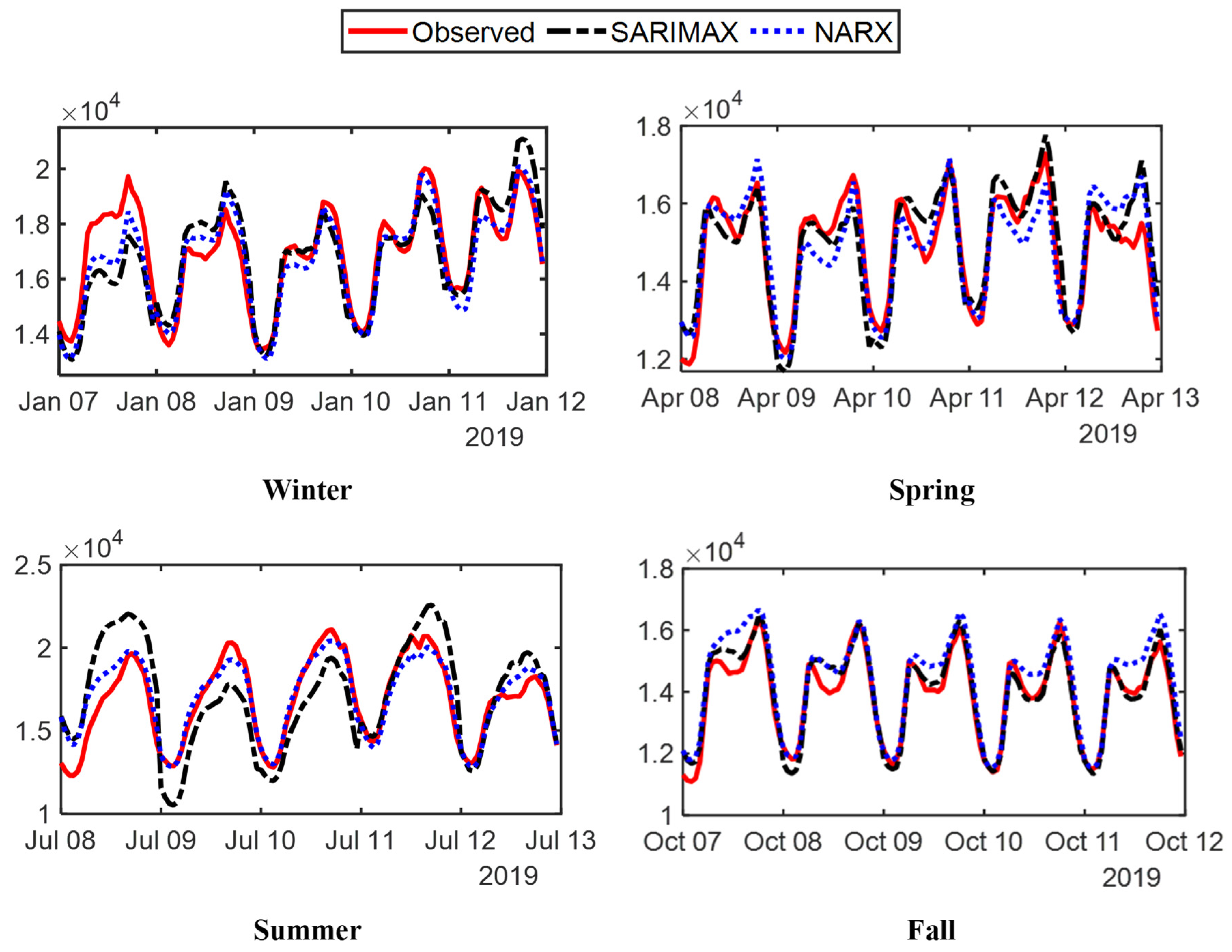
4.3. Performance Evaluation and Model Comparison

The developed hybrid BOA-SARIMAX and BOA-NARX models were tested for day-ahead forecasting of five consecutive weekdays in four seasons of 2019. The average MAE, RMSE, MAPE, ${\mathrm{R}}^2$, adj-R² and FB values for all five testing weekdays are displayed in

Table 4. MAE, RMSE, MAPE, ${\mathrm{R}}^2$, $\mathrm{adj} {\mathrm{R}}^2$, and FB for five testing days in four seasons of 2019.

		MAE (MW)	RMSE (MW)	MAPE (MW)	${\mathbf{R}}^2$	$\mathbf{Adj}-{\mathbf{R}}^2$	FB
BOA-SARIMAX	January 2019	825.1307	945.8183	4.7468	0.9719	0.9641	0.0101
	April 2019	469.5054	573.8192	3.2249	0.9499	0.9360	−0.0059
	July 2019	1735.5	1910	10.4028	0.9635	0.9534	−0.0058
	October 2019	256.5279	303.7495	1.8782	0.9869	0.9833	−0.0059
BOA-NARX	January 2019	553.0839	614.9764	3.2299	0.9687	0.9600	0.0168
	April 2019	471.7548	555.9796	3.1555	0.9512	0.9377	0.0005
	July 2019	610.4919	719.0792	3.7649	0.9674	0.9584	−0.0112
	October 2019	480.9545	570.1857	3.4114	0.96179	0.9512	−0.0325

.

The performance comparisons of the historical data and forecasted electricity demand of all five testing weekdays are shown in Figure 12. Clearly, both models demonstrate the promising ability to handle the day-ahead electricity load forecasts. The forecasted curves presented by the models closely follow the load shapes of several weekdays and describe the peak load changes against various meteorological conditions.

According to Table 4, the prediction performance of the BOA-NARX model is more stable and robust, for example, the average MAPE of five consecutive weekdays for all seasons in the BOA-NARX model is about 3%, while in the BOA-SARIMAX model, there is a remarkable variation in the value of averaged MAPE between the seasons. However, an outstanding prediction of the BOA-SARIMAX model (MAPE = 1.8782, ${\mathrm{R}}^2$= 0.9869, adj-R² = 0.9833, FB = −0.0059) compared to BOA-NARX model (MAPE = 3.4114, ${\mathrm{R}}^2=$0.96179, adj-R² = 0.9512, FB = −0.0325) was observed for the selected days in the Fall season. For load uncertainty, the performance gap between the BOA-SARIMAX model and the BOA-NARX model was most considerable in Summer, which had the highest peak load and the highest part of the uncertainty. This is intuitively reasonable, as the BOA-SARIMAX model is made of a linearity assumption, whereas the true temporal association and covariance are primarily nonlinear. Moreover, the considerable uncertainty in the time-series electricity load data may greatly reduce the performance of the BOA-SARIMAX model since regression-based approaches guess that both input and output parameters follow the Gaussian distribution. Overall, the BOA-NARX model reveals the most favorable and steady ability to handle the day-ahead electricity load forecasts. Several studies reported that the NARX model works excellently in forecasting [51,52]. Our results are in agreement with these studies.

An hour-of-day indexed error analysis was conducted for all four seasons to analyze how the BOA-NARX model improves day-ahead load predictions compared to the BOA-SARIMAX model. The averaged absolute relative errors (%) of five consecutive testing days at each hour of the day for both models are shown in Figure 13. As shown in Figure 13, there are remarkable variations in the absolute relative errors throughout the day in all seasons except Summer. In Summer, there is not much variation in the hourly forecasting errors of the models in the first few hours, whereas these values evolve quite differently across the day. A significant increase in error starts from hour 12, when the BOA-SARIMAX model is employed. The relative error for the BOA-SARIMAX model is comparatively low (range 0.73~2.98%) in Fall and very high (range 8.41~14.44%) in Summer. On the other hand, the BOA-NARX model shows an overall steady result in all seasons (range about 1~6.56%). However, regarding the computation efficiency, the BOA-SARIMAX model shows higher efficiency (average 74.138 s/run) than the BOA-NARX model (average 1832.465 s/run).

Although the studies reported in Table 4 have various time ranges, overall, one can see that with ~3% of average MAPE values of the tested period for all seasons, the BOA-NARX tests aligned with [25] and outperformed [34,36]. All these findings thus support other studies published elsewhere [53].

Further, to confirm the prediction accuracy, a robustness analysis was performed. In this regard, three sets of manipulated testing datasets were created by introducing three different noise levels into the day-ahead weather data. Specifically, for the five-day hourly weather profile (5 × 24 = 120 data points), 20%, 40%, and 60% of the original data points were manipulated with the Gaussian distributed white noise. The SARIMAX and NARX models were re-run on the noise-introduced datasets.

Table 5. Averaged MAE, RMSE, and MAPE values for five testing days in January 2019 under different noise levels.

	BOA-SARIMAX			BOA-NARX
Percentage of Introduced Noise	MAE	RMSE	MAPE	MAE	RMSE	MAPE
0%	825.1307	945.8183	4.7468	553.0839	614.9764	3.2299
20%	825.1293	945.8161	4.7468	553.3542	615.2964	3.2314
40%	825.2115	945.9330	4.7473	554.3769	616.0434	3.2371
60%	825.4104	946.3487	4.7482	562.3439	620.1726	3.2773

shows the averaged MAE, RMSE, and MAPE values for five testing days under different noise levels. It is indicated that, with the introduction of up to 60% white noise, the average MAPE values of the SARIMAX and NARX models increase slightly from 4.7468 to 4.7482 and from 3.2299 to 3.2773, respectively. Therefore, it is verified that both models are robust in terms of forecasting. However, the prediction accuracy of the BOA-NARX model is much better than that of the BOA-SARIMAX model.

4.4. Practical Applications and Prospects

Although a significant improvement in model development (both statistical and machine learning-based) for forecasting electricity demand has been made, analyzing the short-term electricity demand in Canada is still limited. While some predictive models offer exceptional capability in handling complex nonlinear relationships, model complexity, computation efficiency, and robustness are of concern. It is noteworthy that model performance greatly depends on its hyperparameters; thus, automatically tuning these parameters is crucial to achieving an optimum model with less computational effort. In this regard, substantial time, research, and experiments (computational trials) are required for a particular dataset. Hence, such a modeling approach is not only a state-of-the-art application, but also a potential area of study. To the authors’ knowledge, most energy research articles overlook the auto-tuning process to optimize hyperparameters. In this regard, the Bayesian optimization algorithm (BOA) could play an important role. As a result, a powerful hybrid platform (BOA + statistical method or BOA + artificial intelligence approach) may build, which could be effective in terms of generating excellent and robust predictions.

5. Conclusions

In this study, the residential electricity demand for 2013–2019 in Ontario, Canada, was analyzed. The neighborhood component analysis was performed to select six significant weather-related features, namely snow depth, cloud cover, precipitation, temperature, irradiance toa, and irradiance surface. Hybrid BOA-SARIMAX and BOA-NARX models were developed for forecasting the short-term electricity demand. The performances of the models were compared using several performance indicators. Both models’ predicted data for all tested periods almost overlapped on historical values (R² > 0.96). BOA-NARX provides the average MAPE of the tested period for all seasons of ~3%, while BOA-SARIMAX significantly deviates between the seasons. A steady RE at each hour of the day was found (1~6.56%) in BOA-NARX for all seasons, while unstable variations (Fall: 0.73~2.98%; Summer: 8.41~14.44%) were observed in BOA-SARIMAX. The BOA-SARIMAX model showed higher computation efficiency compared to the BOA-NARX model. The overall results indicated that the performances of both models were comparable. However, the developed BOA-NARX model had a better prediction accuracy and stability performance than the BOA-SARIMAX model. It can be concluded that the developed predictive platform successfully estimated the electricity consumption; thus, it could be a potential tool for policymakers to deliver favorable insights into forecasting and improving energy strategies.

References

1. Raza, M.Q.; Khosravi, A. A Review on Artificial Intelligence Based Load Demand Forecasting Techniques for Smart Grid and Buildings. Renew. Sustain. Energy Rev. 2015, 50, 1352–1372. [Google Scholar] [CrossRef]
2. Kuster, C.; Rezgui, Y.; Mourshed, M. Electrical Load Forecasting Models: A Critical Systematic Review. Sustain. Cities Soc. 2017, 35, 257–270. [Google Scholar] [CrossRef]
3. Yang, D.; Guo, J.E.; Li, J.; Wang, S.; Sun, S. Knowledge Mapping in Electricity Demand Forecasting: A Scientometric Insight. Front. Energy Res. 2021, 9, 633. [Google Scholar] [CrossRef]
4. Al-Ghandoor, A.; Jaber, J.O.; Al-Hinti, I.; Mansour, I.M. Residential Past and Future Energy Consumption: Potential Savings and Environmental Impact. Renew. Sustain. Energy Rev. 2009, 13, 1262–1274. [Google Scholar] [CrossRef]
5. Hu, Z.; Bao, Y.; Xiong, T. Electricity Load Forecasting Using Support Vector Regression with Memetic Algorithms. Sci. World J. 2013, 2013, 292575. [Google Scholar] [CrossRef]
6. Alfares, H.K.; Nazeeruddin, M. Electric Load Forecasting: Literature Survey and Classification of Methods. Int. J. Syst. Sci. 2010, 33, 23–34. [Google Scholar] [CrossRef]
7. Shah, I.; Iftikhar, H.; Ali, S. Modeling and Forecasting Medium-Term Electricity Consumption Using Component Estimation Technique. Forecasting 2020, 2, 163–179. [Google Scholar] [CrossRef]
8. Shah, I.; Iftikhar, H.; Ali, S.; Wang, D. Short-Term Electricity Demand Forecasting Using Components Estimation Technique. Energies 2019, 12, 2532. [Google Scholar] [CrossRef] [Green Version]
9. Velasquez, C.E.; Zocatelli, M.; Estanislau, F.B.; Castro, V.F. Analysis of Time Series Models for Brazilian Electricity Demand Forecasting. Energy 2022, 247, 123483. [Google Scholar] [CrossRef]
10. Javed, U.; Ijaz, K.; Jawad, M.; Ansari, E.A.; Shabbir, N.; Kütt, L.; Husev, O. Exploratory Data Analysis Based Short-Term Electrical Load Forecasting: A Comprehensive Analysis. Energies 2021, 14, 5510. [Google Scholar] [CrossRef]
11. Bu, S.J.; Cho, S.B. Time Series Forecasting with Multi-Headed Attention-Based Deep Learning for Residential Energy Consumption. Energies 2020, 13, 4722. [Google Scholar] [CrossRef]
12. Alam, M.S.; Sultana, N.; Hossain, S.M.Z.; Islam, M.S. Hybrid Intelligence Modeling for Estimating Shear Strength of FRP Reinforced Concrete Members. Neural Comput. Appl. 2022, 34, 7069–7079. [Google Scholar] [CrossRef]
13. Sultana, N.; Hossain, S.M.Z.; Abusaad, M.; Alanbar, N.; Senan, Y.; Razzak, S.A. Prediction of Biodiesel Production from Microalgal Oil Using Bayesian Optimization Algorithm-Based Machine Learning Approaches. Fuel 2022, 309, 122184. [Google Scholar] [CrossRef]
14. Hossain, S.M.Z.; Sultana, N.; Razzak, S.A.; Hossain, M.M. Modeling and Multi-Objective Optimization of Microalgae Biomass Production and CO2 Biofixation Using Hybrid Intelligence Approaches. Renew. Sustain. Energy Rev. 2022, 157, 112016. [Google Scholar] [CrossRef]
15. Bouktif, S.; Fiaz, A.; Ouni, A.; Serhani, M.A. Optimal Deep Learning LSTM Model for Electric Load Forecasting Using Feature Selection and Genetic Algorithm: Comparison with Machine Learning Approaches. Energies 2018, 11, 1636. [Google Scholar] [CrossRef] [Green Version]
16. Singh, N.; Mohanty, S.R.; Shukla, R.D. Short Term Electricity Price Forecast Based on Environmentally Adapted Generalized Neuron. Energy 2017, 125, 127–139. [Google Scholar] [CrossRef]
17. Lee, J.; Cho, Y. National-Scale Electricity Peak Load Forecasting: Traditional, Machine Learning, or Hybrid Model? Energy 2022, 239, 122366. [Google Scholar] [CrossRef]
18. Khodayar, M.; Liu, G.; Wang, J.; Khodayar, M.E. Deep Learning in Power Systems Research: A Review. CSEE J. Power Energy Syst. 2020, 7, 209–220. [Google Scholar] [CrossRef]
19. Shahriari, B.; Swersky, K.; Wang, Z.; Adams, R.P.; De Freitas, N. Taking the Human out of the Loop: A Review of Bayesian Optimization. Proc. IEEE 2016, 104, 148–175. [Google Scholar] [CrossRef] [Green Version]
20. Owoyele, O.; Pal, P.; Torreira, A.V.; Probst, D.; Shaxted, M.; Wilde, M.; Senecal, P.K. Application of an Automated Machine Learning-Genetic Algorithm (AutoML-GA) Coupled with Computational Fluid Dynamics Simulations for Rapid Engine Design Optimization. Int. J. Engine Res. 2021, 14680874211023466. [Google Scholar] [CrossRef]
21. Kaboli, S.H.A.; Selvaraj, J.; Rahim, N.A. Long-Term Electric Energy Consumption Forecasting via Artificial Cooperative Search Algorithm. Energy 2016, 115, 857–871. [Google Scholar] [CrossRef]
22. Rehman, S.A.U.; Cai, Y.; Fazal, R.; Das Walasai, G.; Mirjat, N. An Integrated Modeling Approach for Forecasting Long-Term Energy Demand in Pakistan. Energies 2017, 10, 1868. [Google Scholar] [CrossRef] [Green Version]
23. Kankal, M.; Uzlu, E. Neural Network Approach with Teaching—Learning-Based Optimization for Modeling and Forecasting Long-Term Electric Energy Demand in Turkey. Neural Comput. Appl. 2017, 28, 737–747. [Google Scholar] [CrossRef]
24. Khan, A.; Chiroma, H.; Imran, M.; Khan, A.; Bangash, J.I.; Asim, M.; Hamza, M.F.; Aljuaid, H. Forecasting Electricity Consumption Based on Machine Learning to Improve Performance: A Case Study for the Organization of Petroleum Exporting Countries (OPEC). Comput. Electr. Eng. 2020, 86, 106737. [Google Scholar] [CrossRef]
25. Yukseltan, E.; Yucekaya, A.; Bilge, A.H. Hourly Electricity Demand Forecasting Using Fourier Analysis with Feedback. Energy Strateg. Rev. 2020, 31, 100524. [Google Scholar] [CrossRef]
26. Bedi, J.; Toshniwal, D. Empirical Mode Decomposition Based Deep Learning for Electricity Demand Forecasting. IEEE Access 2018, 6, 49144–49156. [Google Scholar] [CrossRef]
27. AL-Musaylh, M.S.; Deo, R.C.; Adamowski, J.F.; Li, Y. Short-Term Electricity Demand Forecasting Using Machine Learning Methods Enriched with Ground-Based Climate and ECMWF Reanalysis Atmospheric Predictors in Southeast Queensland, Australia. Renew. Sustain. Energy Rev. 2019, 113, 109293. [Google Scholar] [CrossRef]
28. Chapagain, K.; Kittipiyakul, S.; Kulthanavit, P. Short-Term Electricity Demand Forecasting: Impact Analysis of Temperature for Thailand. Energies 2020, 13, 2498. [Google Scholar] [CrossRef]
29. Adeboye, A.; Xu, B.; Erik, R.T.; Tamara, O. COVID-19 and the Impact on Energy Consumption: An Environmental Assessment of Ontario Canada. Int. J. Sci. Res. Publ. 2020, 10, 857–865. [Google Scholar] [CrossRef]
30. Al-Musaylh, M.S.; Deo, R.C.; Adamowski, J.F.; Li, Y. Short-Term Electricity Demand Forecasting with MARS, SVR and ARIMA Models Using Aggregated Demand Data in Queensland, Australia. Adv. Eng. Inform. 2018, 35, 1–16. [Google Scholar] [CrossRef]
31. Ouda, M.; El-Nakla, S.; Yahya, C.B.; Omar Ouda, K.M. Electricity Demand Forecast in Saudi Arabia. In Proceedings of the 2019 IEEE 7th Palestinian International Conference on Electrical and Computer Engineering (PICECE), Gaza, Palestine, 26–27 March 2019. [Google Scholar]
32. Abdel-Aal, R.E.; Al-Garni, A.Z. Forecasting monthly electric energy consumption in eastern Saudi Arabia using univariate time-series analysis. Energy 1997, 22, 1059–1069. [Google Scholar] [CrossRef]
33. Liu, N.; Babushkin, V.; Afshari, A. Short-Term Forecasting of Temperature Driven Electricity Load Using Time Series and Neural Network Model. J. Clean Energy Technol. 2014, 2, 327–331. [Google Scholar] [CrossRef]
34. Shadkam, A. Using Sarimax to Forecast Electricity Demand and Consumption in University Buildings. Ph.D. Thesis, University of British Columbia, Vancouver, BC, Canada, 2020. [Google Scholar]
35. Buitrago, J.; Asfour, S. Short-Term Forecasting of Electric Loads Using Nonlinear Autoregressive Artificial Neural Networks with Exogenous Vector Inputs. Energies 2017, 10, 40. [Google Scholar] [CrossRef] [Green Version]
36. AL-Musaylh, M.S.; Deo, R.C.; Li, Y. Electrical Energy Demand Forecasting Model Development and Evaluation with Maximum Overlap Discrete Wavelet Transform-Online Sequential Extreme Learning Machines Algorithms. Energies 2020, 13, 2307. [Google Scholar] [CrossRef]
37. Boussaada, Z.; Curea, O.; Remaci, A.; Camblong, H.; Bellaaj, N.M. A Nonlinear Autoregressive Exogenous (NARX) Neural Network Model for the Prediction of the Daily Direct Solar Radiation. Energies 2018, 11, 620. [Google Scholar] [CrossRef] [Green Version]
38. Sultana, N.; Hossain, S.M.Z.; Taher, S.; Khan, A.; Razzak, S.A.; Haq, B.; Al Shehri, D. Modeling and Optimization of Non-Edible Papaya Seed Waste Oil Synthesis Using Data Mining Approaches. S. Afr. J. Chem. Eng. 2020, 33, 151–159. [Google Scholar] [CrossRef]
39. Hossain, S.M.Z.; Sultana, N.; Jassim, M.S.; Coskuner, G.; Hazin, L.M.; Razzak, S.A.; Hossain, M.M. Soft-Computing Modeling and Multiresponse Optimization for Nutrient Removal Process from Municipal Wastewater Using Microalgae. J. Water Process Eng. 2022, 45, 102490. [Google Scholar] [CrossRef]
40. Guzman, S.M.; Paz, J.O.; Tagert, M.L.M. The Use of NARX Neural Networks to Forecast Daily Groundwater Levels. Water Resour. Manag. 2017, 31, 1591–1603. [Google Scholar] [CrossRef]
41. Lin, T.; Horne, B.G.; Tino, P.; Giles, C.L. Learning Long-Term Dependencies in NARX Recurrent Neural Networks. IEEE Trans. Neural Netw. 1996, 7, 1329–1338. [Google Scholar] [CrossRef] [Green Version]
42. Lin, T.; Horne, B.; Tiño, P.; Giles, C. Learning Long-Term Dependencies Is Not as Difficult with NARX Networks. In Proceedings of the Advances in Neural Information Processing Systems, Denver, CO, USA, 27–30 November 1995; pp. 577–583. [Google Scholar]
43. Lin, T.; Horne, B.G.; Giles, C.L. How Embedded Memory in Recurrent Neural Network Architectures Helps Learning Long-Term Temporal Dependencies. Neural Netw. 1998, 11, 861–868. [Google Scholar] [CrossRef]
44. Wunsch, A.; Liesch, T.; Broda, S. Groundwater Level Forecasting with Artificial Neural Networks: A Comparison of Long Short-Term Memory (LSTM), Convolutional Neural Networks (CNNs), and Non-Linear Autoregressive Networks with Exogenous Input (NARX). Hydrol. Earth Syst. Sci. 2021, 25, 1671–1687. [Google Scholar] [CrossRef]
45. Wunsch, A.; Liesch, T.; Broda, S. Forecasting Groundwater Levels Using Nonlinear Autoregressive Networks with Exogenous Input (NARX). J. Hydrol. 2018, 567, 743–758. [Google Scholar] [CrossRef]
46. Alsumaiei, A.A. A Nonlinear Autoregressive Modeling Approach for Forecasting Groundwater Level Fluctuation in Urban Aquifers. Water 2020, 12, 820. [Google Scholar] [CrossRef] [Green Version]
47. Snoek, J.; Larochelle, H.; Adams, R.P. Practical Bayesian Optimization of Machine Learning Algorithms. In Proceedings of the Advances in Neural Information Processing Systems, Lake Tahoe, NV, USA, 3–6 December 2012. [Google Scholar]
48. Wu, J.; Chen, X.-Y.; Zhang, H.; Xiong, L.-D.; Lei, H.; Deng, S.-H. Hyperparameter Optimization for Machine Learning Models Based on Bayesian Optimizationb. J. Electron. Sci. Technol. 2019, 17, 26–40. [Google Scholar] [CrossRef]
49. Rasmussen, C.E. Gaussian Processes for Machine Learning: Book Webpage; MIT Press: Cambridge, MA, USA, 2006. [Google Scholar]
50. Sultana, N. Predicting Sun Protection Measures against Skin Diseases Using Machine Learning Approaches. J. Cosmet. Dermatol. 2022, 21, 758–769. [Google Scholar] [CrossRef]
51. Koschwitz, D.; Frisch, J.; van Treeck, C. Data-Driven Heating and Cooling Load Predictions for Non-Residential Buildings Based on Support Vector Machine Regression and NARX Recurrent Neural Network: A Comparative Study on District Scale. Energy 2018, 165, 134–142. [Google Scholar] [CrossRef]
52. Abdel Daiem, M.M.; Hatata, A.; Said, N. Modeling and Optimization of Semi-Continuous Anaerobic Co-Digestion of Activated Sludge and Wheat Straw Using Nonlinear Autoregressive Exogenous Neural Network and Seagull Algorithm. Energy 2022, 241, 122939. [Google Scholar] [CrossRef]
53. Cai, M.; Pipattanasomporn, M.; Rahman, S. Day-Ahead Building-Level Load Forecasts Using Deep Learning vs. Traditional Time-Series Techniques. Appl. Energy 2019, 236, 1078–1088. [Google Scholar] [CrossRef]
Figure 1. Average yearly electricity consumption in Ontario from 2013 to 2018 (note that the pandemic period, after 2018 onward, is purposely excluded to avoid any bias created by repetitive lockdowns and consequent increases in residential demand).
Energies 15 03425 g001
Figure 2. Overall flow chart of the methodology.
Energies 15 03425 g002
Figure 3. Trend analysis plot for yearly electricity load (PJ) in 2013–2019.
Energies 15 03425 g003
Figure 4. Typical daily load profiles in winter, spring, Summer, and fall.
Energies 15 03425 g004
Figure 5. Typical daily load profiles over two weeks.
Energies 15 03425 g005
Figure 6. Feature ranking based on the neighborhood component analysis.
Energies 15 03425 g006
Figure 7. ACF and PACF plots of hourly energy load.
Energies 15 03425 g007
Figure 8. Residual diagnostic plots of the developed SARIMAX model.
Energies 15 03425 g008
Figure 9. NARX networks for (a) open loop and (b) closed loop architectures.
Energies 15 03425 g009
Figure 10. Performance plot of the developed neural network.
Energies 15 03425 g010
Figure 11. Regression plot of the developed NARX model.
Energies 15 03425 g011
Figure 12. Comparison of observed and day-ahead forecasted electricity loads (MW) for five testing days in four seasons of 2019 using SARIMAX and NARX algorithm.
Energies 15 03425 g012
Figure 13. Average relative errors (%) at each hour of the day for five testing days in four seasons of 2019 based on SARIMAX and NARX model.
Energies 15 03425 g013